LARGE-SCALE IMAGE RETRIEVAL USING SIMILARITY PRESERVING BINARY CODES
Yunchao Gong
A dissertation submitted to the faculty of the University of North Carolina at Chapel Hill in partial fulfillment of the requirements for the degree of Doctor of Philosophy in
the Department of Computer Science.
Chapel Hill 2014
c
2014
ABSTRACT
YUNCHAO GONG: LARGE-SCALE IMAGE RETRIEVAL USING SIMILARITY PRESERVING BINARY CODES.
(Under the direction of Svetlana Lazebnik.)
Image retrieval is a fundamental problem in computer vision, and has many appli-cations. When the dataset size gets very large, retrieving images in Internet image collections becomes very challenging. The challenges come from storage, computation speed, and similarity representation. My thesis addresses learning compact similarity preserving binary codes, which represent each image by a short binary string, for fast retrieval in large image databases.
to millions of dimensions. I develop a novel method for converting such descriptors to compact similarity-preserving binary codes that exploits their natural matrix structure to reduce their dimensionality using compact bilinear projections instead of a single large projection matrix. This method achieves retrieval and classification accuracy comparable to that of the original descriptors and to the state-of-the-art Product Quantization ap-proach while having orders of magnitude faster code generation time and smaller memory footprint.
ACKNOWLEDGMENTS
First, I would like to express my sincere gratitude to my advisor, Professor Svetlana Lazebnik, for her great support of my Ph.D. research. She introduced me to the area of computer vision, shaped me as a serious researcher, taught me to always focus on challenging problems, and to always try to make an impact. In particular, from her I learned the benefits of critical thinking and striving for perfection. I have been very lucky to have Lana as my advisor, and this dissertation could not have been accomplished without her guidance. I am also grateful to my wonderful thesis committee members: Professor Dinesh Manocha, Professor Alexander C. Berg, Professor Jan-Michael Frahm, Professor Marc Niethammer, and Dr. Sanjiv Kumar.
valuable opportunity to work on the world’s largest brain-simulation system. I also thank Dr. Sergey Ioffe for serving as my mentor for my Google Ph.D. Fellowship, and for his many helpful suggestions.
Great work cannot be done without great collaborators. I am lucky to have worked with many smart colleagues. I especially thank Ruiqi Guo for his critical (and interest-ing!) comments about my work throughout my doctoral studies. I also thank many other collaborators and coauthors: Dr. Joseph Tighe, Dr. Sanjiv Kumar, Dr. Henry Rowley, Dr. Qifa Ke, Dr. Michael Isard, Dr. Albert Gordo, Dr. Florent Perronnin, Dr. Vishal Verma, Dr. Yangqing Jia, Dr. Thomas Leung, Dr. Sergey Ioffe, Dr. Alexander Toshev, Dr. Julia Hockenmaier, Felix X. Yu, Liwei Wang, and Micah Hodosh.
TABLE OF CONTENTS
LIST OF FIGURES . . . xi
LIST OF TABLES . . . .xiv
CHAPTER 1: Introduction . . . .1
1.1 Overview of Contributions . . . .6
CHAPTER 2: Related Works . . . 10
2.1 Approximate Nearest Neighbor Search . . . 10
2.1.1 Spatial Partitioning Tree and Locality Sensitive Hashing . . . 11
2.1.2 Similarity Preserving Binary Codes . . . 13
2.1.3 Product Quantization . . . 19
2.2 Large-scale Image Retrieval and Recognition. . . 20
2.2.1 Internet Computer Vision and Beyond . . . 23
CHAPTER 3: Iterative Quantization for Learning Compact Binary Codes . . . 26
3.1 The ITQ Formulation . . . 27
3.1.1 Dimensionality Reduction . . . 28
3.1.2 Binary Quantization . . . 30
3.2 Evaluation of Unsupervised Code Learning . . . 33
3.2.1 Datasets. . . 33
3.2.4 Results on 580,000 Tiny Images . . . 39
3.2.5 Evaluation of Hashing Performance . . . 43
3.3 ITQ with a Kernel Embedding . . . 47
3.3.1 Random Fourier Features . . . 47
3.3.2 Results . . . 48
3.4 Discussion . . . 51
CHAPTER 4: Angular Quantization for Histogram Data . . . 53
4.1 Angular Quantization-based Binary Codes . . . 55
4.1.1 Data-independent Binary Codes . . . 55
4.1.2 Learning Data-dependent Binary Codes . . . 59
4.1.3 Optimization . . . 63
4.1.4 Computation of cosine Similarity between Binary Codes . . . 65
4.2 Experiments . . . 65
4.2.1 Datasets and Protocols. . . 65
4.2.2 Results on SUN and ImageNet . . . 67
4.2.3 Results on 20 Newsgroups. . . 68
4.2.4 Timing . . . 73
4.3 Discussion . . . 74
CHAPTER 5: Bilinear Hashing for Very High-dimensional Data. . . 75
5.1 Bilinear Binary Codes . . . 78
5.1.1 Learning Bilinear Binary Codes . . . 80
5.2 Experiments . . . 86
5.2.1 Datasets and Features. . . 86
5.2.2 Experimental Protocols . . . 88
5.2.3 Baseline Methods . . . 89
5.2.4 Code Generation Time and Storage . . . 90
5.2.5 Retrieval on Holiday+Flickr1M . . . 91
5.2.6 Retrieval on ILSVRC2010 with VLAD . . . 95
5.2.7 Retrieval on ILSVRC2010 with LLC . . . 96
5.2.8 Image Classification . . . 97
5.3 Discussion . . . 100
CHAPTER 6: Combining Semantic Embeddings and Binary Codes . . . 103
6.1 Semantic Binary Codes for Weakly Tagged Data. . . 104
6.1.1 Results on Tiny Images . . . 106
6.1.2 Results on NUS-WIDE Dataset . . . 108
6.2 Binary classeme . . . 112
6.3 Discussion . . . 118
CHAPTER 7: Hashing Revisited: Observations and Open Problems. . . 120
7.1 Why Do Binary Codes Work? . . . 121
7.2 Distance Function Matters . . . 123
7.3 Neighborhood Definition Matters . . . 130
CHAPTER 8: Discussion and Future Directions . . . 138
8.1 Summary of Contributions . . . 138
8.2 Future Directions. . . 139
LIST OF FIGURES
1.1 Visual search for shopping . . . .2
1.2 Illustration of visual similarity. . . .3
1.3 Mapping images to binary codes. . . .4
2.1 Toy example of kd-tree and LSH.. . . 11
3.1 Toy example of ITQ . . . 27
3.2 ITQ optimization . . . 32
3.3 Main results for ITQ . . . 38
3.4 NN search results on CIFAR dataset for ITQ. . . 40
3.5 Semantic retrieval results on CIFAR dataset for ITQ. . . 41
3.6 NN search results on Tiny images for ITQ. . . 42
3.7 Overview of NN results on Tiny images for ITQ. . . 43
3.8 Qualitative results for ITQ . . . 44
3.9 NN search hashing results for ITQ . . . 45
3.10 Semantic hashing results for ITQ . . . 46
3.11 Kernel ITQ results. . . 49
3.12 Kernel ITQ with different radius results . . . 50
4.1 Quantization model in 3D . . . 56
4.2 cosine of angle between binary vertices . . . 59
4.4 Results on SUN dataset . . . 69
4.5 Results on ImageNet120K . . . 70
4.6 Results on 20 Newsgroups . . . 71
4.7 Effect of projection on Hamming weight. . . 72
5.1 Memory of projections vs. dimensionality . . . 76
5.2 Visualization of the distribution of the VLAD descriptor . . . 84
5.3 Sample images from Holiday Dataset. . . 87
5.4 Results on Holiday dataset . . . 93
5.5 Results on ILSVRC with VLAD feature . . . 94
5.6 Results on ILSVRC with LLC feature . . . 98
5.7 Sample image retrieval results . . . 101
6.1 Logical flow of the PCA+ITQ and CCA+ITQ methods. . . 106
6.2 Semantic retrieval results on CIFAR. . . 108
6.3 Sample image retrieval results on CIFAR . . . 109
6.4 Sample image search results on NUS dataset . . . 113
6.5 Data flow of the binary classeme idea. . . 114
6.6 Qualitative results for text to image search 2 on NUS-WIDE . . . 115
6.7 Sample image search results on ImageNet . . . 119
7.1 Analysis of the distribution on Hamming cube . . . 122
7.3 A comparison of different random hashing models. . . 127
7.4 Comparison of different random hash models . . . 128
7.5 Visualization of a toy dataset. . . 130
7.6 Analysis of the distribution of the neighbors . . . 133
7.7 Comparison of different methods on different neighborhood definitions. . . 134
7.8 The distribution of neighbors for different queries . . . 135
LIST OF TABLES
4.1 Semantic retrieval results on SUN dataset . . . 68
4.2 Semantic retrieval results on ImageNet120K dataset . . . 68
4.3 Semantic retrieval results on 20 Newsgroups dataset . . . 73
4.4 Timing for binary codes . . . 73
5.1 Code generation time for linear and bilinear projections. . . 90
5.2 Memory needed to store projections . . . 90
5.3 Running time on ILSVRC . . . 92
5.4 Image classification results on ILSVRC . . . 99
6.1 Image retrieval results on NUS-WIDE . . . 111
6.2 Image retrieval results on ILSVRC . . . 116
CHAPTER 1: Introduction
We interact with images every day. We use Google Image Search to find interesting images, and we upload our personal photos to Facebook, which contains billions of images contributed by its users. Mobile applications for image retrieval are available, including Google Goggles, a mobile-image-search tool that provides real-time image search results. Google Shopping also provides visually similar items (e.g., Figure 1.1) to improve the shopping experience. Clearly, Internet photo collections have become one of the most important parts of everyday life. However, how to organize such collections is still an open problem in computer vision research, and in order to address it, we must first address the problem of large-scale similarity search.
Today, image search and recognition research is being performed on ever-larger databases. For example, the ImageNet database (Deng et al., 2009) currently contains around 15M images and 20K categories. The main challenges for large-scale image retrieval are:
1. How to define similarity between images;
2. How to design compact representations for images, so we can store them;
3. How to design fast search schemes, so we can efficiently find similar images.
Figure 1.1: Image search for shopping applications – finding visually similar items. Image taken from Google Shopping.
feature vector, and directly compute the distance between these vectors, which is referred to as feature similarity. A good feature similarity should reflect semantic similarity: i.e. that images containing the same objects or scenes should have smaller distance, and images containing different objects or scenes should have larger distance, as shown in Figure 1.2. Defining good feature representations reflecting this semantic similarity is one of the major challenges of recognition in general, but it is not my primary focus. For the most part of this thesis, I will assume that the feature representation is given and fixed, and try to design binary codes that preserve both feature-space and semantic similarity in that representation.
similar dissimilar
Figure 1.2: An illustration of visual similarity. Images containing same object should be more similar to images containing different objects.
Binary encoding
1011001011…0101 1110101101…0010 0001111000…1010
1111111001…0001
1010101010…1001 0001111110…1010 0101101001…1111 1001111000…1010 0001001001…0010 1001110010…1010 1101111000…0010
1101111001…0001
Similar images ||x – y|| 0
Binary encoding
0001111000…1010 1111111001…0001
1010101010…1001 0001111110…1010 0101101001…1111 1001111000…1010 0001001001…0010 1001110010…1010 1101111000…0010 1101111001…0001 0001111000…0010 0010011011…1111 Dissimilar images
||x – y|| is large
(a) Similar images have similar binary codes
(b) dissimilar images have dissimilar binary codes
Figure 1.3: Mapping images to similarity-preserving short binary codes, so distances between images are measured by fast Hamming distance. (a) Similar images x and y
should have similar binary codes with small Hamming distance. (b) Dissimilar imagesx
underlying theoretical guarantees for using very large numbers of random projections to preserve the geometry of high-dimensional data. Not all LSH schemes yield binary embeddings of data, however. Torralba et al. (2008b) have introduced the binary coding problem to the vision community and have compared several methods based on boosting, restricted Boltzmann machines (Salakhutdinov and Hinton, 2009), and LSH. Such work opens a new avenue for LSH and its applications in computer vision, especially because it tries to answer the question of how to learn compact binary codes from real data, so that such codes can be used in real applications. Considerable attention has been devoted to this problem, subsequently (Weiss et al., 2008; Rahimi and Recht, 2007; Raginsky and Lazebnik, 2009; Wang et al., 2010a) as well as applications that show the promise of binary codes for vision problems (Frahm et al., 2010; Kuettel et al., 2012).
1.1 Overview of Contributions
is described in Chapter 3.
underlying representation.
My second extension of ITQ in Chapter 5 is motivated by recent the success of the Fisher vector (FV) (Perronnin and Dance, 2007; Perronnin et al., 2010b) and vector of locally aggregated descriptor (VLAD) (J´egou et al., 2010) – very powerful visual descrip-tors that have achieved state-of-the-art performance for visual retrieval and recognition. However, the dimensionality of FV and VLAD is extremely high and the feature is dense, which makes it very hard to perform learning and retrieval. The high dimensionality also makes mapping it to binary codes very inefficient. There are two major problems: first, the projection matrix will be extremely large, and may not even fit in memory; second, the projection speed will become extremely slow due to the multiplication with the huge projection matrix. To solve these two problems, I propose a bilinear formulation that uses two small projections to reconstruct the huge projection matrix. This approach ad-dresses both the storage and projection speed problems. My experiments on large-scale image retrieval and classification datasets (J´egou et al., 2008; Deng et al., 2009) have demonstrated that my approach offers comparable performance to the original dense FV or VLAD, with a much more compact representation and faster retrieval speed.
bi-nary codes work as well as the original real embedding for large-scale retrieval problems in Internet image collections.
CHAPTER 2: Related Works
This chapter contains a survey of important works related to this thesis. In Section 2.1, I will present a survey on approximate nearest neighbor search and similarity pre-serving binary codes. In Section 2.2, I review relevant work in our key application areas of large-scale image classification and retrieval.
2.1 Approximate Nearest Neighbor Search
Nearest neighbor search (Shakhnarovich et al., 2006; Samet, 1990) is a fundamental operation underlying many computer vision approaches. Brute-force search, which means comparing a query point with every point in the database, becomes prohibitively expen-sive as the dataset size and the dimensionality of the features grow. To reduce search com-plexity, a number of algorithms and data structures have been proposed (Shakhnarovich et al., 2006). These methods can be broadly categorized into two classes:
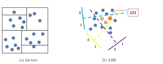
• Spatial partitioning methods such as trees (Bentley, 1975; Samet, 1990) and hash tables (Andoni and Indyk, 2008), which are aimed at enabling sublinear-time sim-ilarity search;
(a) kd-tree
0
1
0
1
0 1
101
(b) LSH
Figure 2.1: A toy example of kd-tree and LSH scheme. (a) kd-tree partitions the space by recursively partitioning the coordinates. (b) LSH partitions the space by random projections. (Figure (b) is from Professor Rob Fergus’s slides.)
2.1.1 Spatial Partitioning Tree and Locality Sensitive Hashing
Tree- and hashing-based nearest neighbor search has been an active research area in theoretical computer science, machine learning, and computer vision. These methods partition the feature space into a large number of cells and try to achieve sub-linear searches by reducing the search space.
neighbors. However, kd-trees suffer from the curse of dimensionality and cannot handle high-dimensional data (e.g., several hundred dimensions). A few other tree variants such ask-means trees (Nister and Stewenius, 2006) and random projection trees (Freund et al., 2007) have also been applied to nearest neighbor search in vision applications, but have achieved limited success for high-dimensional data.
2.1.2 Similarity Preserving Binary Codes
Unlike tree-based methods and LSH, similarity preserving binary codes (Torralba et al., 2008b; Weiss et al., 2008; Gong and Lazebnik, 2011b) do not necessarily offer sub-linear search complexity. However, they can reduce memory requirements and the running times of brute-force searches by significant, constant factors, and they do not involve building and maintaining complex data structures.
The similarity preserving binary code idea was first introduced by Salakhutdinov and Hinton (2009) for text retrieval, and then introduced to the vision community by Torralba et al. (2008b). Both of these researchers used a deep neural network architecture to learn binary codes and were able to show successful applications for text, image retrieval, and scene parsing. A number of subsequent works that are surveyed in the following pages focused on designing better models for learning binary codes. Most methods considered here consist of the following three steps:
1. Projection learning, or finding a linear or nonlinear projection of the data;
2. Binary thresholding, or quantizing continuous projected data to binary vectors;
3. Similarity computation, or finding distances between query and database points.
I will discuss each of these steps in related methods in the next sections.
Step 1: Projection Learning
nonlinear projection to reduce data dimensionality. One example is the angle-preserving LSH scheme by Charikar (2002); Andoni and Indyk (2008) that uses hyperplanes to preserve angles. Kulis and Grauman (2009); Kulis et al. (2009) generalized this LSH formulation to the setting in which the similarity is given by a “black-box” kernel function. Raginsky and Lazebnik (2009) used random Fourier features (Rahimi and Recht, 2007) to approximate the Gaussian kernel. All of these methods are based on random projections. With large numbers of random projections, these methods usually enjoy strong theoretical guarantees for approximating the distance between the original points; however, when the number of bits is small, they tend to be quite noisy. Therefore they might not be appropriate for applications with limited storage budgets.
(Gordo et al., 2011; J´egou et al., 2011) also used PCA as an initial step for the projection step. Gordo et al. (2011) proposed to directly threshold PCA projections, and have obtained good performance with asymmetric distance computation (see below). J´egou et al. (2011) also applied PCA in their image retrieval pipeline for fast indexing. Beyond PCA, He et al. (2011) used a method similar to independent component analysis (ICA) for learning hash functions; they showed that such projections usually do not need to be coupled with an “adjustment” because ICA projections are learned to be independent. Strecha et al. (2010) used linear discriminant analysis (LDA) and Liu et al. (2012) used discriminative graph embedding to learn supervised hash codes that work better for semantic retrieval. In my work, I start with PCA projections. In Chapter 3 I will show how to adjust these projections for better preservation of similarities.
Step 2: Binary Thresholding
hashing (Weiss et al., 2008, 2012), allocated bits based on separable Laplacian eigenfunc-tions, but the allocation function was heuristic and involved very restricted assumptions about the data. The work by Liu et al. (2011) similarly used multiple bits per dimension to address the imbalanced variance problem. Norouzi and Fleet (2012); Norouzi et al. (2012a) proposed an elegant structured prediction framework to directly minimize the error of quantization through structured learning, which was solved by optimizing the upper bound of the structured loss. The methods Norouzi and Fleet (2012); Norouzi et al. (2012a) do not split the projection learning and quantization stage, but instead directly learn the hash functions, and have achieved superior performance. However, one limitation is that such approaches usually involve many free parameters that must be tuned.
In this thesis, I proposed approaches that directly try to minimize binary quantization error by learning a rotation of PCA-projected data and have achieved state-of-the-art performance. Some other approaches have also proposed other methods for thresholding. Heo et al. (2012) proposed to use hyperspheres instead of hyperplanes to partition the space. Some recent works (Kong and Li, 2012; Ge et al., 2013; Norouzi and Fleet, 2013) adopted the rotation learning idea of ITQ and further improved it.
Step 3: Distance Computation for Binary Codes
asymmetric distance.
Most methods directly compute the Hamming distance between the respective binary codes, which simply measures how many bits are different between two strings. Hamming distance can be computed very efficiently using XOR and POPCOUNT operation in CPU. For example, given two binary vectors b1 = 1001 and b2 = 0011, their XOR is computed as:
1 0 0 1
⊕ 0 0 1 1 1 0 1 0,
and then the internal CPU operation POPCOUNT is used to count the number of 1s in the resulting vector to obtain the Hamming distance. In practice, we can group 64 bits together to a unsigned 64-bit integer, and during distance computation we can directly perform operations on the integers.
The second method iscosine similarity between binary codes. The cosine of the angle θ between two binary vectorsb1 and b2 is defined as:
cos(θ) = b
T
1b2
kb1k2kb2k2
. (2.1)
The dot-product bT1b2 can be obtained by bitwise AND followed by POPCOUNT, and
kb1k2 and kb2k2 can be obtained by popcount and lookup table to find the square root. Of course, if b1 is the query vector that needs to be compared to every database vector
the original data vectors.
The third method isasymmetric distance(Dong et al., 2008; Gordo et al., 2011; J´egou et al., 2011), in which the database points are quantized but the query data point is not. Such an approach usually offers better performance than Hamming distance. However, the query data structure is also more complicated and the search speed is not as fast as that of Hamming distance. For a query x ∈ Rc (x has been rotated or transformed
by hash function without binarization) and database points b ∈ {−1,+1}c, the lower-bounded asymmetric distance is simply the L2 distance between x and b: da(x,b) =
kxk2
2 +c−2xTb. Since kxk22 is on the query side and c is fixed, in practice, we only need to compute xTb. We can do this by putting bits in groups of 8 and constructing a 1×256 lookup table to make the dot-product computation more efficient.
The three different functions introduced above will be used in following chapters. In particular, Hamming distance will be used in Chapter 3 and Chapter 6, cosine similarity will be used in Chapter 4, and asymmetric distance will be used in Chapter 5.
2.1.3 Product Quantization
most accurate baselines in the literature.
2.2 Large-scale Image Retrieval and Recognition
The main applications of similarity preserving binary codes in my thesis are large-scale image classification and retrieval. These in turn can serve as the bases for many other applications where binary codes can be useful, such as location recognition (Hays and Efros, 2008), scene parsing (Tighe and Lazebnik, 2010), object detection (Felzenszwalb et al., 2008), image segmentation (Kuettel et al., 2012), 3D reconstruction (Frahm et al., 2010), and many others.
Several large-scale datasets (Deng et al., 2009; Xiao et al., 2010; Torralba et al., 2008a) have recently become the new benchmarks for recognition and retrieval research. ImageNet (Deng et al., 2009) is arguably the most important web-scale image dataset; currently, it contains around 15M images and 20K categories. All the images in that database have been manually verified and labeled with WordNet (Miller, 1995) categories. The SUN dataset (Xiao et al., 2010) is the largest dataset for scene recognition,with 397 categories and more than 100,000 images. The 80M tiny-images dataset (Torralba et al., 2008a) is the largest publicly available dataset, though it suffers from poor image quality and noisy annotations.
that a data-independent mapping usually works comparably to (if not better than) a data-dependent one. Both the nonlinear embedding methods and the feature coding schemes result in representations that are extremely high-dimensional.
difficult. Several recent works have experimented with methods for compressing VLAD. For example, Perronnin et al. (2011) have investigated binary coding methods includ-ing spectral hashinclud-ing (Weiss et al., 2008) and LSH (Andoni and Indyk, 2008). J´egou et al. (2010) proposed a joint dimensionality reduction and coding method that first performs PCA to reduce dimensionality, and then performs product quantization (J´egou et al., 2011) to convert the data to the compressed domain. Subsequent works by J´egou and Chum (2012) proposed several simple improvements, such as whitened PCA, which further reduce the dimensionality and improve performance.
Throughout this thesis, I will perform retrieval and recognition using a variety of visual descriptors. In Chapter 3, I will start with the relatively low-dimensional GIST descriptor (Oliva and Torralba, 2001) which is the most commonly used feature for evalu-ating binary coding methods. Accordingly, I will develop specific binary coding methods for BoW type data in Chapter 4, and for very high dimensional descriptors (e.g. VLAD and LLC) in Chapter 5.
2.2.1 Internet Computer Vision and Beyond
noisily-tagged Internet image collections. Another popular way to obtain an intermedi-ate embedding space for images is by mapping them to outputs of a bank of concepts or attribute classifiers (Rasiwasia et al., 2007; Wang et al., 2009b; Farhadi et al., 2009). This is related to the idea of classeme representation (Torresani et al., 2010). I will also demonstrate an application that converts classemes to binary codes in Chapter 6. There are many other applications as well for which cleanly labeled training data may be scarce (Guillaumin et al., 2010; Quattoni et al., 2007; Wang et al., 2009a). This is a weakly supervised setting (as opposed to the fully supervised setting (Deng et al., 2009; Perronnin et al., 2010b)), where the idea is to use a large amount of noisy data to improve the classification results on a small, clean training set. The methods I present in Chapter 6 are also useful for learning from weakly tagged data.
methods have also achieved success in annotation tasks involving Internet-scale datasets. Perhaps the largest-scale discriminative image-annotation system in the literature is the WSABIE (web scale annotation by image embedding) system proposed by Weston et al. (2011). It uses a stochastic gradient descent to optimize a ranking objective function and has been evaluated on datasets with 10M training examples. Because most of the annotation methods use nearest neighbor as an important component, binary codes can be used to improve their efficiency.
CHAPTER 3: Iterative Quantization for Learning Compact Binary Codes
This Chapter details my Iterative Quantization (ITQ) algorithm, which will also serve as the foundation for the methods of Chapters 4 and 5. ITQ was mainly inspired by the work by Weiss et al. (2008) and Wang et al. (2010a), which both use principal component analysis (PCA) to reduce the dimensionality of the data prior to binary coding. However, since the variance of the data in each PCA direction is different (and in particular, higher-variance directions carry much more information), encoding each direction with the same number of bits is bound to produce poor performance.
−1 0 1 −1
0 1
Average quantization error: 1.00
(a) PCA aligned.
−1 0 1
−1 0 1
Average quantization error: 0.93
(b) Random Rotation.
−1 0 1
−1 0 1
Average quantization error: 0.88
(c) Optimized Rotation.
Figure 3.1: Toy illustration of my ITQ method (see Section 3.1 for details). The basic binary encoding scheme is to quantize each data point to the closest vertex of the binary cube, (±1,±1) (this is equivalent to quantizing points according to their quadrant). (a) The x and yaxes correspond to the PCA directions of the data. Note that quantization assigns points in the same cluster to different vertices. (b) Randomly rotated data – the variance is more balanced and the quantization error is lower. (c) Optimized rotation found by ITQ – quantization error is lowest, and the partitioning respects the cluster structure.
concern theunsupervised setting, that does not use labeled data to learn binary codes. In Chapter 6, I will show applications that use label information to learn binary codes. This work was originally published in Gong and Lazebnik (2011b) and Gong et al. (2013c).
3.1 The ITQ Formulation
Let me first define notations. We have a set ofndata points{x1,x2, . . . ,xn},xi ∈Rd,
that form the rows of the data matrix X ∈ Rn×d. The goal is to learn a binary code
matrix B ∈ {−1,1}n×c, where c denotes the code length. Each row of B is denoted
as bi. For each bit k = 1, . . . , c, the binary encoding function is usually defined by
hk(x) = sgn(xwk), where wk is a column vector of hyperplane coefficients and
sgn(v) =
1, if v ≥0;
−1, otherwise.
For a matrix or a vector, sgn(·) will denote the result of element-wise application of the above function. Thus, we can write the entire encoding process as:
B = sgn(XW), (3.1)
where W ∈ Rd×c is the matrix with columns w
k. We assume that the points are
zero-centered, i.e., Pn
i=1xi = 0.
3.1.1 Dimensionality Reduction
pairwise uncorrelated. We can do this by maximizing the following objective function:
I(W) = X
k
var(hk(x)) =
X
k
var(sgn(xwk)),
1 nB
TB =I .
As shown in Wang et al. (2010a), the variance is maximized by encoding functions that produce exactly balanced bits, i.e., when hk(x) = 1 for exactly half of the data points
and −1 for the other half. However, the requirement of exact balancedness makes the above objective function intractable. Adopting the same signed magnitude relaxation as in Wang et al. (2010a), we get the following continuous objective function:
e
I(W) = X
k
E(kxwkk22) = 1 n
X
k
wTkXTXwk
= 1
ntr(W
TXTXW), WTW =I . (3.2)
The constraint WTW = I requires the hashing hyperplanes to be orthogonal to each
3.1.2 Binary Quantization
Let v ∈ Rc be a vector in the projected space. It is easy to show (see below) that sgn(v) is the vertex of the hypercube{−1,1}cclosest tov in terms of Euclidean distance.
The smaller the quantization loss ksgn(v)−vk2, the better the resulting binary code will preserve the original locality structure of the data. Now, going back to eq. (3.2), it is clear that if W is an optimal solution, then so is Wf =W R for any orthogonal c×c
matrix R. Therefore, we are free to orthogonally transform the projected dataV =XW in such a way as to minimize the quantization loss
Q(B, R) =kB−V Rk2F, (3.3)
where k · kF denotes the Frobenius norm.
The idea of rotating the data to minimize quantization loss can be found in J´egou et al. (2010). However, the approach of J´egou et al. (2010) is based not on binary codes, but on product quantization with asymmetric distance computation (ADC). Unlike in my formulation, direct minimization of quantization loss for ADC is impractical, so J´egou et al. (2010) instead suggest solving an easier problem, that of finding a rotation (or, more precisely, an orthogonal transformation) to balance the variance of the different dimensions of the data. In practice, they find that a random rotation works well for this purpose. Based on this observation, a natural baseline for my method is given by initializing R to a random orthogonal matrix.
I call ITQ to find a local minimum of the quantization loss (3.3). In each iteration, each data point is first assigned to the nearest vertex of the binary hypercube, and then R is updated to minimize the quantization loss given this assignment. These two alternating steps are described in detail below.
Fix R and update B. Expanding (3.3), we have
Q(B, R) = kBk2F +kVk2F −2 tr(BRTVT)
= nc+kVk2F −2 tr(BRTVT). (3.4)
Because the projected data matrix V = XW is fixed, minimizing (3.4) is equivalent to maximizing
tr(BRTVT) =
n
X
i=1
c
X
j=1
BijVeij,
where Veij denote the elements of Ve = V R. To maximize this expression with respect
to B, I need to have Bij = 1 whenever Veij ≥ 0 and −1 otherwise. In other words,
B = sgn(V R) as claimed in the beginning of this section.
0 100 200 300 400 500 1.565 1.57 1.575 1.58 1.585
1.59x 10
6
Number of iterations
Q
(
B
,R
)
(a) Quantization error for 32-bit.
100,0000 300,000 500,000 10
20 30 40 50
number of training data
running time (seconds)
PCA+ITQ PCA+RR PCA+Nonorth SKLSH SH
(b) Training time for 32-bit code.
Figure 3.2: The behavior of ITQ quantization error and training time for a 32-bit code.
the binary cube.
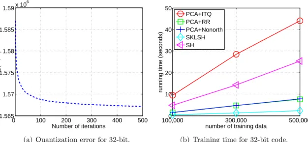
Fix B and update R. For a fixed B, the objective function (3.3) corresponds to the classic Orthogonal Procrustes problem (Schonemann, 1966), in which one tries to find a rotation to align one point set with another. In my case, the two point sets are given by the projected data V and the target binary code matrix B. For a fixed B, (3.3) is minimized as follows: first compute the SVD of the c×cmatrix BTV as SΩ ˆST =BTV and then let R= ˆSST.
We alternate between updates to B and R for several iterations to find a locally optimal solution. The typical behavior of the error (3.3) is shown in Figure 3.2 (a). In practice, I have found that it is not necessary to iterate until convergence to achieve good performance, and I use 50 iterations for all experiments. Figure 3.2 (b) shows the training time for 32-bit code. I have found all the methods scale linearly with the number of images. Although my method takes a slightly longer time, it is still very practical.
discretizing relaxed solutions to multi-class spectral clustering, which is based on finding an orthogonal transformation of the continuous eigenvectors to bring them as close as possible to a discrete solution. One important difference between Yu and Shi (2003) and my approach is that Yu and Shi (2003) allows discretization only to the c orthogonal hypercube vertices with exactly one positive entry, while I use all the 2c vertices as
targets. This enables us to learn efficient codes that preserve the locality structure of the data.
3.2 Evaluation of Unsupervised Code Learning
3.2.1 Datasets
I evaluate my method on two subsets of the Tiny Images dataset (Torralba et al., 2008a). Both of these subsets come from Fergus et al. (2009). The first subset is a version of the CIFAR dataset (Krizhevsky, 2009), and it consists of 64,800 images that have been manually grouped into 11 ground-truth classes (airplane, automobile, bird, boat, cat, deer, dog, frog, horse, ship and truck). The second, larger subset consists of 580,000 Tiny Images. Apart from the CIFAR images, which are included among the 580,000 images, all the other images lack manually supplied ground truth labels, but they come associated with one of 388 Internet search keywords. In this section, I will use the CIFAR ground-truth labels to evaluate the semantic consistency of my codes.
resulting in 320-dimensional feature vectors. Because my method (as well as many state-of-the-art methods) cannot use more bits than the original dimension of the data, the evaluation is limited to code sizes up to 256 bits.
3.2.2 Protocols and Baseline Methods
I follow two evaluation protocols widely used in recent papers (Raginsky and Lazebnik, 2009; Wang et al., 2010a; Weiss et al., 2008). The first one is to evaluate performance of nearest neighbor search using Euclidean neighbors as ground truth. As in Raginsky and Lazebnik (2009), a nominal threshold of the average distance to the 50th nearest neighbor is used to determine whether a database point returned for a given query is considered a true positive. Then, based on the Euclidean ground truth, I compute the recall-precision curve and the mean average precision (mAP), or the area under the recall precision curve. In particular, given the predefined ground truth, we rank the database items based on the learned codes, and compute recall and precision. To summarize the curves in a compact form, we directly report the mean average precision (mAP), which measures the area under precision recall curve. We first define average precision for one query,
AveP =
Z 1
0
p(r)dr≈
n
X
k=1
P(k)∆r(k) (3.5)
whereP(k) andr(k) are the values of the precision and recall. The mAP forQ different queries are computed as MAP = PQ
q=1AveP(q)
For this case, I report the averaged semantic precision of the top 500 ranked images for each query as in (Wang et al., 2010b). This measure is reporting the percentage of images having the same class label to the query within the 500 top ranked images. For all experiments, I randomly select 1000 points to serve as test queries. The remaining images form the training set on which the code parameters are learned, as well as the database against which the queries are performed. All the experiments reported in this chapter are averaged over five random training/test partitions.
I compare my ITQ method to three baseline methods that follow the basic hashing scheme H(X) = sgn(XfW), where the projection matrix fW is defined in different ways:
1. LSH: fW is a Gaussian random matrix (Andoni and Indyk, 2008). Note that in
theory, this scheme has locality preserving guarantees only for unit-norm vectors. While I do not normalize the data to unit norm, I have found that it still works well as long as the data is zero-centered.
2. PCA-Direct: fW is simply the matrix of the topc PCA directions. This baseline
is included to show what happens when we do not rotate the PCA-projected data prior to quantization.
3. PCA-RR:fW =W R, whereW is the matrix of PCA directions andRis a random
orthogonal matrix. This is the initialization of ITQ, as described in Section 3.1.2.
I also compare ITQ to three state-of-the-art methods using code provided by the authors:
2. SKLSH(Raginsky and Lazebnik, 2009): This method is based on the random fea-tures mapping for approximating shift-invariant kernels (Rahimi and Recht, 2007). In Raginsky and Lazebnik (2009), this method is reported to outperform SH for code sizes larger than 64 bits. I use a Gaussian kernel with bandwidth set to the average distance to the 50th nearest neighbor as in Raginsky and Lazebnik (2009). 3. PCA-Nonorth (Wang et al., 2010a): Non-orthogonal relaxation of PCA. This method is reported in Wang et al. (2010a) to outperform SH. Note that instead of using semi-supervised PCA as in Wang et al. (2010a), the evaluation of this section uses standard unsupervised PCA since I assume there is no class label information available.
Note that of all the six methods above, LSH and SKLSH are the only ones that rely on randomized data-independent linear projections. All the other methods, including my PCA-RR and PCA-ITQ, use PCA (or a non-orthogonal relaxation of PCA) as an intermediate dimensionality reduction step.
3.2.3 Results on CIFAR Dataset
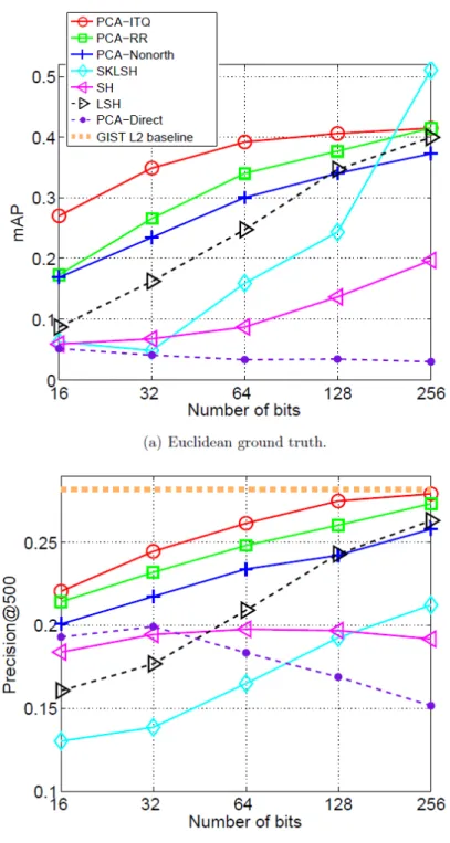
actually decrease in performance as the number of bits increases.
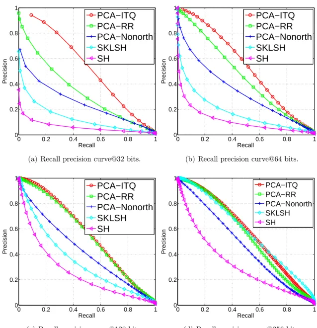
Figures 3.4 and 3.5 show complete recall-precision and class label precision curves corresponding to the summary numbers in Figures 3.3(a,b). To avoid clutter, these curves (and all the subsequent results reported in this chapter) omit the two baseline methods LSH and PCA-Direct. The complete curves confirm the trends seen in Figures 3.3 (a,b). What becomes especially apparent from looking at Figure 3.4(d) is that the data-dependent methods (PCA-Nonorth, PCA-RR, PCA-ITQ) seem to hit a ceiling of performance as code size increases, while the data-independent SKLSH method does not have a similar limitation (in fact, in the limit of infinitely many bits, SKLSH is guaranteed to yield exact Euclidean neighbors). Once again, the message seems to be that adapting binary codes to the data can give the biggest gain for small code sizes.
3.2.4 Results on 580,000 Tiny Images
0 0.2 0.4 0.6 0.8 1 0 0.2 0.4 0.6 0.8 1 Recall Precision PCA−ITQ PCA−RR PCA−Nonorth SKLSH SH
(a) Recall precision curve@32 bits.
0 0.2 0.4 0.6 0.8 1 0 0.2 0.4 0.6 0.8 1 Recall Precision PCA−ITQ PCA−RR PCA−Nonorth SKLSH SH
(b) Recall precision curve@64 bits.
0 0.2 0.4 0.6 0.8 1 0 0.2 0.4 0.6 0.8 1 Recall Precision PCA−ITQ PCA−RR PCA−Nonorth SKLSH SH
(c) Recall precision curve@128 bits.
0 0.2 0.4 0.6 0.8 1 0 0.2 0.4 0.6 0.8 1 Recall Precision PCA−ITQ PCA−RR PCA−Nonorth SKLSH SH
(d) Recall precision curve@256 bits.
0 100 200 300 400 500 0.2
0.3 0.4
Number of top returned images
Precision PCA−ITQ PCA−RR PCA−Nonorth SKLSH SH
(a) Class label precision@32 bits.
0 100 200 300 400 500 0.2
0.3 0.4
Number of top returned images
Precision PCA−ITQ PCA−RR PCA−Nonorth SKLSH SH
(b) Class label precision@64 bits.
0 100 200 300 400 500 0.2
0.3 0.4
Number of top returned images
Precision PCA−ITQ PCA−RR PCA−Nonorth SKLSH SH
(c) Class label precision@128 bits.
0 100 200 300 400 500 0.2
0.3 0.4
Number of top returned images
Precision PCA−ITQ PCA−RR PCA−Nonorth SKLSH SH
(d) Class label precision@256 bits.
0 0.2 0.4 0.6 0.8 1 0 0.2 0.4 0.6 0.8 1 Recall Precision PCA−ITQ PCA−RR PCA−Nonorth SKLSH SH
(a) Recall precision curve@32 bits.
0 0.2 0.4 0.6 0.8 1 0 0.2 0.4 0.6 0.8 1 Recall Precision PCA−ITQ PCA−RR PCA−Nonorth SKLSH SH
(b) Recall precision curve@64 bits.
0 0.2 0.4 0.6 0.8 1 0 0.2 0.4 0.6 0.8 1 Recall Precision PCA−ITQ PCA−RR PCA−Nonorth SKLSH SH
(c) Recall precision curve@128 bits.
0 0.2 0.4 0.6 0.8 1 0 0.2 0.4 0.6 0.8 1 Recall Precision PCA−ITQ PCA−RR PCA−Nonorth SKLSH SH
(d) Recall precision curve@256 bits.
16 32 64 128 256 0
0.1 0.2 0.3 0.4 0.5
Number of bits
mAP
PCA−ITQ PCA−RR PCA−Nonorth SKLSH SH
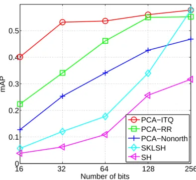
Figure 3.7: mAP on the 580,000 Tiny Image subset. Ground truth is defined by Euclidean neighbors.
Finally, Figure 3.8 shows image retrieval examples.
3.2.5 Evaluation of Hashing Performance
(a) Query (b) PCA-ITQ (c) PCA-RR
Precision: 55.56% Precision: 44.44%
Precision: 55.56% Precision: 36.11%
Precision: 69.44% Precision: 63.89%
0 0.2 0.4 0.6 0.8 1 0 0.2 0.4 0.6 0.8 1 Recall Precision PCA−ITQ PCA−RR PCA−Nonorth SKLSH SH r=0 r=1 r=2
(a) CIFAR, 8 bits
0 0.2 0.4 0.6 0.8 1
0 0.2 0.4 0.6 0.8 1 Recall Precision PCA−ITQ PCA−RR PCA−Nonorth SKLSH SH
(b) CIFAR, 16 bits
0 0.2 0.4 0.6 0.8 1
0 0.2 0.4 0.6 0.8 1 Recall Precision PCA−ITQ PCA−RR PCA−Nonorth SKLSH SH
(c) CIFAR, 32 bits
0 0.2 0.4 0.6 0.8 1
0 0.2 0.4 0.6 0.8 1 Recall Precision PCA−ITQ PCA−RR PCA−Nonorth SKLSH SH r=0 r=1 r=2
(d) Tiny images, 8 bits
0 0.2 0.4 0.6 0.8 1
0 0.2 0.4 0.6 0.8 1 Recall Precision PCA−ITQ PCA−RR PCA−Nonorth SKLSH SH
(e) Tiny images, 16 bits
0 0.2 0.4 0.6 0.8 1
0 0.2 0.4 0.6 0.8 1 Recall Precision PCA−ITQ PCA−RR PCA−Nonorth SKLSH SH
(f) Tiny images, 32 bits
0 0.1 0.2 0.3 0.4 0.5 0.1 0.15 0.2 0.25 Recall Precision PCA−ITQ PCA−RR PCA−Nonorth SKLSH SH r=0 r=1 r=2
(a) CIFAR, 8 bits
0 0.02 0.04 0.06
0.1 0.15 0.2 0.25 Recall Precision PCA−ITQ PCA−RR PCA−Nonorth SKLSH SH
(b) CIFAR, 16 bits
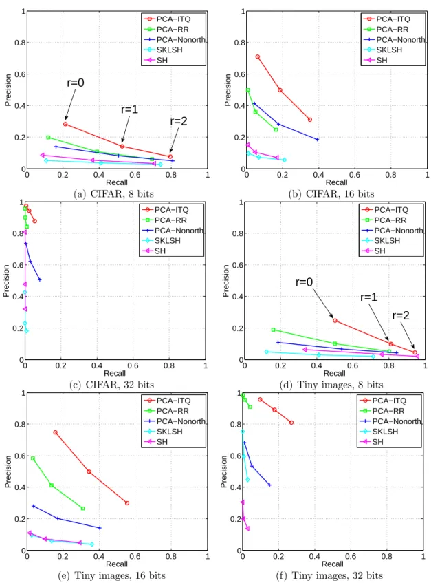
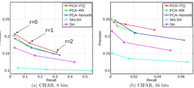
Figure 3.10: Hashing performance on the CIFAR dataset with class label ground truth. r is Hamming radius. Note the progressively decreasing recall from (a) to (c), and the different vertical scale in (c).
order of magnitude.
3.3 ITQ with a Kernel Embedding
3.3.1 Random Fourier Features
A big limitation of PCA is that it can only capture linear structure in the data. In order to introduce nonlinearity into the embedding process, I can use kernel PCA (KPCA) (Scholkopf et al., 1997). Finding the KPCA embedding for n feature vectors involves computing the n×n kernel matrix and performing eigendecomposition on it. However, for large-scale image databases, these operations are prohibitively expensive, so I have to resort to approximation schemes.
In this section, I am particularly interested in the Gaussian kernel, whose radius can be used to control the neighborhood size for nearest-neighbor search. To approximate the Gaussian kernelK(x,y) = exp(−kx−yk2/(2σ2)), I can use the explicit random Fourier feature (RFF) mapping (Rahimi and Recht, 2007). For a data point x, each coordinate of this mapping is given by
Φw,b(x) =
√
2 cos(xw+b),
where the random projection vectorwis drawn from Normal(0,σ12I) andb is drawn from Unif[0,2π]. A D-dimensional embedding is given by
ΦD(x)ΦD(y)T. WhenDgoes to infinity, the mapping becomes exact. In my experiments, I useD= 3,000. After the random Fourier mapping, I simply perform linear PCA on top of ΦD(X) to obtain an approximate KPCA embedding for the data. Given the points
in my dataset, I first transform them using RFF, then perform KPCA to reduce the dimensionality, and finally binarize the data in the same way as before.
Note that while I solely focus on approximation of the Gaussian kernel, there also exist explicit mappings for other popular kernels (Maji et al., 2008; Perronnin et al., 2010a).
3.3.2 Results
0 0.2 0.4 0.6 0.8 1 0
0.2 0.4 0.6 0.8 1
Recall
Precision
KPCA (4δ)
KPCA (2δ)
KPCA (δ)
KPCA (δ/2)
PCA
Figure 3.12: Performance of kernel ITQ (32 bits) with a ground truth radius δ equal to half the distance to the 50th nearest neighbor. The numbers in parentheses show the value of the kernel width σ used in the RFF mapping.
It is interesting to compare KPCA-RR/ITQ and SKLSH (Raginsky and Lazebnik, 2009), since the latter is also based on RFF. To obtain ac-bit code, SKLSH first computes a c-dimensional RFF embedding of the data and then quantizes each dimension after adding a random threshold. By contrast, my KPCA-based methods start with a 3,000-dimensional RFF embedding and then use PCA to reduce it to topc dimensions. Based on the results of Figure 3.11, this process makes an especially big difference for class label precision.
structure of the data. To demonstrate this, I use a ground-truth radius δ defined as half the distance to the 50th nearest neighbor. This results in only very close points (near duplicates) being defined as ground truth neighbors. Figure 3.12 shows recall and precision of KPCA-ITQ for σ = [δ/2, δ, 2δ, 4δ]. The best performance is obtained for δ and δ/2, which match the desired neighborhood size the most closely. By contrast, KPCA-ITQ with a larger radius, or PCA-ITQ, which does not have a radius parameter, work very poorly in this regime.
Let me summarize the benefits of using the RFF embedding in combination with ITQ. First, it allows us to use more bits than original feature dimensions to get better code accuracy. Second, it significantly improves class label precision, especially when combined with CCA. Third, it has a tunable radius parameter that can be changed to obtain much better performance on tasks such as near-duplicate image retrieval.
3.4 Discussion
CHAPTER 4: Angular Quantization for Histogram Data
In many vision and text-related applications, it is common to represent data as a Bag of Words (BoW) (Salton and McGill, 1986; Csurka et al., 2004; Sivic and Zisserman, 2003), or a vector of counts or frequencies, which contains only non-negative entries. Furthermore, cosine of the angle between vectors is typically used as a similarity measure for such data. This chapter presents an extension to the ITQ approach presented in Chapter 3 by exploring the special data distribution of histograms.
works by quantizing each data point to the vertex of the positive orthant of the binary hypercube with which it has the smallest angle. This is very similar to ITQ, but the difference is the definition of landmark points. For ITQ, we define landmark points in
4.1 Angular Quantization-based Binary Codes
4.1.1 Data-independent Binary Codes
We assume we are given a database containing n d-dimensional points {xi}ni=1 as defined in Chapter 3. I first address the problem of computing ad-bit binary code of an input vector xi. A c-bit code for c < d will be described later in Sec. 4.1.2. For
angle-preserving quantization, I define a set of quantization centers or landmarks by projecting the vertices of the binary hypercube{0,1}donto the unit hypersphere. This construction
results in 2d−1 landmark points ford-dimensional data. Note that the vertex with all 0’s is excluded as its norm is 0, which is not permissible in eq. (4.1). An illustration of the proposed quantization model is given in Figure 4.1. Given a pointx on the hypersphere, one first finds its nearest1 landmark vi, and the binary encoding for xi is simply given
by the binary vertex bi corresponding to vi. Since in terms of angle from a point, both
bi and vi are equivalent, I will use the term landmark for either bi or vi depending on
the context.
Figure 4.1: An illustration of my quantization model in 3D. Herebi is a vertex of the unit cube
andviis its projection on the unit sphere. Pointsvi are used as the landmarks for quantization.
To find the binary code of a given data point x, I first find its nearest landmark point vi on
the sphere, and the correponding bi gives its binary code (v4 and b4 in this case).
that performing brute-force neighbor search might even be slower than nearest-neighbor retrieval from the original database! To obtain an efficient solution, I propose to take advantage of the special structure of our set of landmarks, which are given by the projections of binary vectors onto the unit hypercube. The nearest landmark of a point
x, or the binary vertex having the smallest angle with x, is given by
ˆ
b = arg max
b bTx
kbk2
s.t. b∈ {0,1}d. (4.1)
Algorithm 1: Finding the nearest binary landmark for a point on the unit hypersphere. Input: pointxon the unit hypersphere.
Output: ˆb, binary vector having the smallest angle withx. 1. Sort the entries of xin descending order as x(1), . . . , x(d). 2. for k= 1, . . . , d
3. if x(k)= 0 break.
4. Form binary vectorbkwhose elements are 1 for theklargest positions
in x, 0 otherwise.
5. Compute ψ(x, k) = (xTbk)/kbkk2=
Pk
j=1x(j)
/√k.
6. endfor
7. Return bk corresponding tom= arg maxkψ(x, k).
Lemma 1 The globally optimal solution of the integer programming problem in eq. (4.1)
can be computed in O(dlogd) time. Further, for a sparse vector with s non-zero entries, it can be computed in O(slogs) time.
Proof: Since b is a d-dimensional binary vector, its norm kbk2 can have at most d different values, i.e., kbk2 ∈ {
√
1, . . . ,√d}. We can separately consider the optimal solution of eq. (4.1) for each value of the norm. Given kbk2 =
√
k (i.e., b has k ones), eq. (4.1) is maximized by setting to one the entries of b corresponding to the largest k entries of x. Since kbk2 can take on d distinct values, we need to evaluate eq. (4.1) at most d times, and find the k and the corresponding ˆb for which the objective function is maximized (see Algorithm 1 for a detailed description of the algorithm). To find the largest k entries of x for k = 1, . . . , d, We need to sort all the entries of x, which takes O(dlogd) time, and checking the solutions for all k is linear ind. Further, if the vector
helps to characterize the angular resolution of the quantization landmarks.
Lemma 2 Suppose b is an arbitrary binary vector with Hamming weight kbk1 = m, where k · k1 is the L1 norm. Then for all binary vectorsb0 that lie at a Hamming radius
r from b, the cosine of the angle between b and b0 is bounded by hqmm−r,p m m+r
i
.
Proof: Since kbk1 = m, there are exactly m ones in b and the rest are zeros, and b0 has exactly r bits different from b. To find the lower bound on the cosine of the angle between b and b0, we want to find a b0 such that √ bTb0
kbk1√kb0k1 is maximized. It is easy to see that this will happen when b0 has exactly m−r ones in common positions with
b and the remaining entries are zero, i.e., kb0k1 = m−r and bTb 0
=m−r. This gives the lower bound of qmm−r. Similarly, the upper bound can be obtained when b0 has all ones at the same locations asb, and additionalr ones, i.e., kb0k1 =m+r andbTb0 =m. This yields the upper bound of p m
m+r.
10
010
110
210
30
0.2
0.4
0.6
0.8
1
m (log scale)
cos(b
1
,b
2)
lower bound (r=1) upper bound (r=1) lower bound (r=3) upper bound (r=3) lower bound (r=5) upper bound (r=5)
Figure 4.2: Bound on cosine of angle between a binary vertex b1 with Hamming weight m, and another vertexb2 at a Hamming distancer from b1. See Lemma 2 for details.
the distribution of the data should be such that a majority of the points fall closer to landmarks with higher m.
Algorithm 1 constitutes the core of my proposed angular quantization method, but it has several limitations: (i) it is data-independent, and thus cannot adapt to the data distribution to control the quantization error; (ii) it cannot control m which, based on my analysis, is critical for low quantization error; (iii) it can only produce a d-bit code ford-dimensional data, and thus cannot generate shorter codes. In the following section, I present a learning algorithm to address the above issues.
4.1.2 Learning Data-dependent Binary Codes
3, I would like to align the data to a pre-defined set of quantization landmarks using a rotation, because rotating the data does not change the angles – and, therefore, the similarities – between the data points. Later in this section, I will present an objective function and an optimization algorithm to accomplish this goal, but first, by way of motivation, I would like to illustrate how applying even a random rotation to a typical frequency/count vector can affect the Hamming weight m of its angular binary code.
Since we are mostly interested in modeling histogram data that is counts and fre-quencies, I propose to use Zipf’s distribution to generate synthetic data for illustration purposes, as most real world histogram data follows this distribution (Manning and Sch¨utze, 1999; Zipf, 1935). Suppose, for a data vector x, the sorted entries x(1), . . . , x(d) follow Zipf’s law, i.e.,x(k) ∝1/kq, wherek is the index of the entries sorted in descending order, and s is the power parameter that controls how quickly the entries decay. The effective m for x depends directly on the power q: the larger q is, the faster the en-tries of x decay, and the smaller m becomes. More germanely, for a fixed s, applying a random rotation R to x makes the distribution of the entries of the resulting vector RTx more uniform and raises the effective m. Figure 4.3 (a) plots the sorted entries of
x generated from Zipf’s law with s = 0.8. Based on Algorithm 1, I compute the scaled cumulative sums ψ(x, k) =Pk
j=1
x√(j)
k, which are shown in Figure 4.3 (b). Here the
opti-mal m= arg maxkψ(x, k) is relatively low (m= 2). In Figure 4.3 (c), I randomly rotate
the data and show the sorted values of RTx, which become more uniform. Finally, in
Figure 4.3 (d), I show ψ(RTx, k). The Hamming weight m after this random rotation
rotations for this example is 27.36. Thus, even randomly rotating the data tends to lead to finer Voronoi cells and reduced quantization error. Next, it is natural to ask whether we can optimize the rotation of the data to increase the cosine similarities between data points and their corresponding binary landmarks.
I seek a d×d orthogonal transformation R such that the sum of cosine similarities of each transformed data point RTx
i and its corresponding binary landmark bi is
max-imized. Note that after rotation, RTxi may contain negative values but this does not
affect the quantization since the binarization technique described in Algorithm 1 effec-tively suppresses the negative values to 0. Let B ∈ {0,1}d×n denote a matrix whose
columns are given by the bi. Then the objective function for my optimization problem
is given by
Q(B, R) = arg max
B,R n
X
i=1
bTi
kbik2
RTxi s.t. bi ∈ {0,1}d, RTR =Id, (4.2)
where Id denotes thed×d identity matrix.
The above objective function still yields a d-bit binary code for d-dimensional data, while in many real-world applications, a low-dimensional binary code may be preferable. To generate a c-bit code where c < d, I can learn a d× c projection matrix R with orthogonal columns by optimizing the following modified objective function:
Q(B, R) = arg max
B,R n
X
i=1
bTi
kbik2
RTx i
kRTx ik2
0 20 40 60 80 100 0 0.1 0.2 0.3 0.4 0.5 0.6 0.7 0.8 0.9 1
sorted index (k)
data value x
(k)
(a)
0 20 40 60 80 100
0.5 0.6 0.7 0.8 0.9 1 1.1
sorted index (k)
Ψ
(x,k)
m=2
(b)
0 20 40 60 80 100
−3 −2 −1 0 1 2 3
sorted index (k)
after rotation (R
T x)
(k)
(c)
0 20 40 60 80 100
0 1 2 3 4 5 6 7 8 9
sorted index (k)
Ψ
(R
T x,k) m=25
(d)
Figure 4.3: Effect of rotation on Hamming weight m of the landmark corresponding to a particular vector. (a) Sorted vector elements x(k) following Zipf’s law with q = 0.8; (b) Scaled cumulative sumψ(x, k); (c) Sorted vector elements after random rotation; (d) Scaled cumulative
tion), the denominator of the objective function contains kRTxik2 since after projection
kRTx
ik2 6= 1. However, adding this new term to the denominator makes the optimization problem hard to solve. I propose to relax it by optimizing the linear correlation instead of the angle:
Q(B, R) = arg max
B,R n
X
i=1
bTi
kbik2
RTxi s.t. bi ∈ {0,1}c, RTR =Ic. (4.4)
This is similar to eq. (4.2) but the geometric interpretation is slightly different: I am now looking for a projection matrixR to map the d-dimensional data to a lower-dimensional space such that after the mapping, the data has high linear correlation with a set of land-mark points lying on the lower-dimensional hypersphere. Section 4.2 will demonstrate that this relaxation works quite well in practice.
4.1.3 Optimization
The objective function in (4.4) can be written more compactly in a matrix form:
Q(B, Re ) = arg max
e
B,R
Tr(BeTRTX) s.t. RTR=Ic, (4.5)
where Tr(·) is the trace operator, Be is thec×n matrix with columns given bybi/kbik2, and X is the d ×n matrix with columns given by xi. This objective is nonconvex in
e
for each bi separately. Here, the individual sub-problem for eachxi can be written as
ˆ
bi = arg max
bi
bTi
kbik2
(RTxi). (4.6)
Thus, given a pointyi =RTx
i inc-dimensional space, I want to find the vertexbi on the
c-dimensional hypercube having the smallest angle withyi. To do this, I use Algorithm 1 to find bi for each yi, and then normalize each bi back to the unit hypersphere: ebi =
bi/kbik2. This yields each column ofBe. Note that the Be found in this way is the global
optimum for this subproblem.
(2) Fix Be, update R. When Be is fixed, I want to find
ˆ
R = arg max
R Tr(Be
TRTX) = arg max R Tr(R
TX
e
BT) s.t. RTR=Ic. (4.7)
This is a well-known problem and its global optimum can be obtained by polar decom-position (Chen et al., 2011). Namely, I take the SVD of the d ×c matrix XBeT as
XBeT =U SVT, let Uc be the first csingular vectors of U, and finally obtain R=UcVT.
1
2, and then normalizing each column to unit norm. Note that the optimization is also computationally efficient. The first subproblem takes O(nclogc) time while the second one takes O(dc2). This is linear in data dimension d, which enables us to handle very high-dimensional feature vectors.
4.1.4 Computation of cosine Similarity between Binary Codes
We use the cosine similarity between binary codes introduced in Section 2.1.2 as the similarity measure. The cosine similarity between two binary codes can also be very efficiently computed using CPU efficient operations.
4.2 Experiments
4.2.1 Datasets and Protocols
To test the effectiveness of the proposed Angular Quantization-based Binary Codes (AQBC) method, I have conducted experiments on two image datasets and one text dataset. The first image dataset is SUN, which contains 142,169 natural scene images (Xiao et al., 2010). Each image is represented by a 1000-dimensional bag of visual words (BoW) feature vector computed on top of dense SIFT descriptors. The BoW vectors are power-normalized by taking the square root of each entry, which has been shown to improve performance for recognition tasks (Perronnin et al., 2011).
is also used as the local descriptor in this case.
The third dataset is 20 Newsgroups,2 which contains 18,846 text documents and 26,214 words. Tf-idf weighting is used for each text document BoW vector. The fea-ture vectors for all three datasets are sparse, non-negative, and normalized to unit L2 norm. Due to this, Euclidean distance directly corresponds to the cosine similarity as dist2 = 2 − 2 sim. Therefore, in the following, I will talk about similarity and distance interchangeably.
To perform evaluation on each dataset, I randomly sample and fix 2000 points as queries, and use the remaining points as the “database” against which the similarity searches are run. For each query, I define the ground truth neighbors as all the points within the radius determined by the average distance to the 50th nearest neighbor in the dataset, and plot precision-recall curves of database points ordered by decreasing similarity of their binary codes with the query. This methodology is similar to our protocol in Chapter 3, and to that of other recent works (Raginsky and Lazebnik, 2009; Weiss et al., 2008). Since my AQBC method is unsupervised, I compare with several state-of-the-art unsupervised binary coding methods: Locality Sensitive Hashing (LSH) (Charikar, 2002), Spectral Hashing (Weiss et al., 2008), ITQ (Chapter 3), Shift-invariant Kernel LSH (SKLSH) (Raginsky and Lazebnik, 2009), and Spherical Hashing (SPH) (Heo et al., 2012). Although these methods are designed to work with the Euclidean distance, they can be directly applied here since all the vectors have unit norm. As in Chapter 3, we also evaluate the semantic precision for binary codes in this section. For this evaluation,
we use ITQ as the main baseline. We follow the experimental protocols mentioned above, and use precision@50 to evaluate different methods. This metric reports the percentage of images having the same class label to each query image within its 50 nearest neighbors.
4.2.2 Results on SUN and ImageNet
code size
16
32
64
128
256
512
1024
ITQ
2.64 3.30 4.22 5.28 5.64 5.91
6.22
AQBC
2.22 2.95 3.58 4.36 5.00 5.97
5.46
Table 4.1: Semantic retrieval results (precision@50) on SUN dataset.
code size
16
32
64
128
256
512
1024
ITQ
6.37 8.33 11.09 12.95 14.09 14.84 15.15
AQBC
5.78 7.44
9.61
11.68 13.12 13.86 14.43
Table 4.2: Semantic retrieval results (precision@50) on ImageNet120K dataset.
results in Table 4.1 and Table 4.2. We can find the proposed AQBC method is usually slightly worse than ITQ. This suggests that using cosine similarity might not have a very significant advantage in terms of semantic retrieval on these datasets. The best distance preserving approach might not be able to lead to the best semantic retrieval performance, and it depends on specific applications.
4.2.3 Results on 20 Newsgroups
0 0.2 0.4 0.6 0.8 1 0 0.2 0.4 0.6 0.8 1 Recall Precision ITQ LSH SKLSH SH SPH AQBC
(a) 64 bits.
0 0.2 0.4 0.6 0.8 1
0 0.2 0.4 0.6 0.8 1 Recall Precision ITQ LSH SKLSH SH SPH AQBC
(b) 256 bits.
0 0.2 0.4 0.6 0.8 1
0 0.2 0.4 0.6 0.8 1 Recall Precision ITQ LSH SKLSH SH SPH AQBC AQBC naive
(c) 1000 bits.
0 0.2 0.4 0.6 0.8 1 0 0.2 0.4 0.6 0.8 1 Recall Precision ITQ LSH SKLSH SH SPH AQBC
(a) 64 bits.
0 0.2 0.4 0.6 0.8 1
0 0.2 0.4 0.6 0.8 1 Recall Precision ITQ LSH SKLSH SH SPH AQBC
(b) 256 bits.
0 0.2 0.4 0.6 0.8 1
0 0.2 0.4 0.6 0.8 1 Recall Precision ITQ LSH SKLSH SH SPH AQBC
(c) 1024 bits.
0 0.2 0.4 0.6 0.8 1 0 0.2 0.4 0.6 0.8 1 Recall Precision ITQ LSH SKLSH SH SPH AQBC
(a) 64 bits.
0 0.2 0.4 0.6 0.8 1
0 0.2 0.4 0.6 0.8 1 Recall Precision ITQ LSH SKLSH SH SPH AQBC
(b) 256 bits.
0 0.2 0.4 0.6 0.8 1
0 0.2 0.4 0.6 0.8 1 Recall Precision ITQ LSH SKLSH SH SPH AQBC
(c) 1024 bits.
Figure 4.6: Precision-recall curves for different methods on the 20 Newsgroups dataset. decays more slowly than the original distribution in Figure 4.7 (a). Figure 4.7 (d) shows the scaled cumulative sum for the projected vectors, indicating a much higher m.