Research Article
3D Pattern Synthesis of Time-Modulated Conformal Arrays with
a Multiobjective Optimization Approach
Wentao Li,
1Yongqiang Hei,
2Jing Yang,
1and Xiaowei Shi
1 1School of Electronic Engineering, Xidian University, Xi’an, Shaanxi 710071, China2State Key Laboratory of Integrated Services Networks, Xidian University, Xi’an, Shaanxi 710071, China Correspondence should be addressed to Wentao Li; [email protected]
Received 28 November 2013; Revised 24 April 2014; Accepted 28 April 2014; Published 2 June 2014 Academic Editor: Atsushi Mase
Copyright © 2014 Wentao Li et al. This is an open access article distributed under the Creative Commons Attribution License, which permits unrestricted use, distribution, and reproduction in any medium, provided the original work is properly cited. This paper addresses the synthesis of the three-dimensional (3D) radiation patterns of the time-modulated conformal arrays. Due to the nature of periodic time modulation, harmonic radiation patterns are generated at the multiples of the modulation frequency in time-modulated arrays. Thus, the optimization goal of the time-modulated conformal array includes the optimization of the sidelobe level at the operating frequency and the sideband levels (SBLs) at the harmonic frequency, and the design can be regarded as a multiobjective problem. The multiobjective particle swarm optimization (MOPSO) is applied to optimize the switch-on instants and pulse duratiswitch-ons of the time-modulated cswitch-onformal array. To significantly reduce the optimizatiswitch-on variables, the modified Bernstein polynomial is employed in the synthesis process. Furthermore, dual polarized patch antenna is designed as radiator to achieve low cross-polarization level during the beam scanning. A 12×13 (156)-element conical conformal microstrip array is simulated to demonstrate the proposed synthesis mechanism, and good results reveal the promising ability of the proposed algorithm in solving the synthesis of the time-modulated conformal arrays problem.
1. Introduction
Conformal phased arrays will prove their potential applica-tions in a variety of fields, such as airborne, missile, and unmanned aerial vehicles, due to their excellent aerodynamic performances [1–3]. However, due to the influences of curved carriers, the design of conformal arrays also faces many challenges. Unlike planar and linear arrays, the radiating elements of conformal arrays generally orient in different directions on curved surfaces, posing unique challenges in the synthesis of antenna arrays. In particular, the cross-polarization level of the conformal phased array is more serious compared with the planar or linear arrays.
With the development of high-speed computers, the synthesis of conformal arrays has made a series of pro-gresses. Bucci et al. proposed a conformal array synthesis procedure which incorporates near-field constraints [4]. In 2005, Boeringer and Werner presented an approach to curved phased array synthesis using the particle swarm optimization with a modified Bernstein polynomial to obtain the excitation
amplitudes [5]. However, during the design process, many practical factors were not considered. In 2007, Vaskelainen used a constrained least-squares method to synthesize con-formal arrays and the least mean square (LMS) error of the constrained least-squares optimization problem has been studied [6]. In 2010, Fuchs proposed a procedure for the synthesis of shaped beams, which reduced the synthesis problem to a linear programming one. A cylindrical array of8 × 8elements was utilized to illustrate the effectiveness of the method, but the optimality of the solution could not be guaranteed [7]. Similarly, Tsui and Chan used iterative second-order cone programming method for the power or shaped beam pattern synthesis of narrowband conformal arrays [8].
However, for the synthesis of patterns with low/ultra-low sidelobes of the conventional conformal arrays, the obtained dynamic range ratios of amplitude excitations could be quite high, which results in stringent requirements on various error tolerances for practical implementation. With the rapid development of engineering technology, the
previously proposed time-modulated antenna array (TMAA) causes the researchers’ attention again [9]. By introducing a fourth dimension—time—into conventional arrays, the feed network of the antenna array can be simplified greatly. Moti-vated by this, introducing the “time-modulated” technology into the conformal phased array will provide a new design approach.
Compared with the conventional array, in time-modu-lated array, each antenna element is connected with a high-speed RF switch which works periodically. Due to the periodic modulation of switches, the inherent property of time-modulated antenna arrays is the presence of sidebands or harmonic signals at the multiples of the time modulation frequency. The sideband signals result in a reduction of the array gain. Aiming at improving the gain of TMAAs and suppressing the sideband levels (SBL), various stochastic optimization algorithms have been used, such as the par-ticle swarm optimization (PSO), genetic algorithm (GA), simulated annealing, differential evolution algorithm, and artificial bee colony algorithm [10–13]. Recently, to improve the gain of TMAAs, a novel approach is proposed by using single-pole-double-throw switches [14], and the concept of a time-modulated reflector array has been analyzed in [15]. In [16], the pulse shaping has been employed as an additional degree of freedom to yield a nonnegligible effect on reduction of the sideband losses. Furthermore, the total power radiated in harmonics for asymmetric pulse distributions has been studied in [17]. However, sideband signals can also be uti-lized. At different sideband frequencies, the time-modulated antenna array can produce multiple beams simultaneously and point at different angular directions [18,19].
In this paper, the synthesis of the three-dimensional (3D) radiation patterns in full space of the time-modulated conformal arrays is investigated. Due to the multiobjective nature of the optimization problem, considering both the SLL at the operating frequency and the sideband levels (SBLs), simultaneously, the multiobjective particle swarm optimization (MOPSO) is employed. To reduce the opti-mization variables and accelerate the speed of convergence, the modified Bernstein polynomial is extended to 3D case in synthesizing conformal arrays. Furthermore, in order to control the polarization of the array during scanning, a dual fed stacked microstrip antenna is designed to build the con-ical conformal array. Finally, a12 × 13(156)-element conical conformal phased array has been successfully simulated.
The remainder of the paper is organized as follows.
Section 2 briefly explains the formulation of the problem.
Section 3presents the detailed architecture of the proposed
algorithm. Numerical results are discussed inSection 4, while
Section 5concludes this paper.
2. Problem Formulation
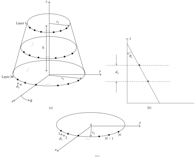
Consider an array of𝑀 × 𝑁elements located over a conical surface, as shown in Figure 1, where 𝑀 and 𝑁 represent the number of elements in the𝑧-direction and𝜑-direction, respectively. The radii of the cone at the top and bottom are denoted as𝑟1= 2.29𝜆and𝑟2= 3.85𝜆, respectively. The height
of the cone isℎ = 5.48𝜆and the half cone angle is𝜃𝑐 = 16∘. The elements are arranged according to the following rule: the space between consecutive horizontal rows is𝑑𝑧 = 0.5𝜆in the𝑧-direction; that is, the elements in the same column are along the same generatrix; the distance between the adjacent elements on the bottom layer is𝑑𝑙= 0.67𝜆.
The far-field radiation pattern produced by these𝑀 × 𝑁 elements placed on the conical surface can be expressed as
FF(𝜃, 𝜑) = 𝑀 ∑ 𝑚=1 𝑁 ∑ 𝑁=1 𝐼𝑚𝑛𝑓𝑚𝑛(𝜃, 𝜑)
×exp[𝑗𝑘𝑟𝑛[sin𝜃𝑐sin𝜃cos(𝜑 − 𝜑𝑚𝑛)
−cos𝜃cos𝜃𝑐] + 𝑗𝜓𝑚𝑛] , (1)
where𝐼𝑚𝑛 is the element excitation current amplitude,𝜓𝑚𝑛 is the excitation current phase, 𝑓𝑚𝑛(𝜃, 𝜑) is the individual element pattern, and𝑟𝑛 is the radius of circle, on which the
𝑚𝑛th element is placed.𝑘is the free-space wave number. The excitation current phase𝜓𝑚𝑛can be calculated by
𝜓𝑚𝑛= −𝑘𝑟𝑛[sin𝜃𝑐sin𝜃0cos(𝜑0− 𝜑𝑚𝑛) −cos𝜃𝑐cos𝜃0] , (2) where(𝜃0, 𝜑0)is the desired steering angle.
In time-modulated arrays, each element is controlled by a high speed RF switch which works periodically. In each modulation period𝑇𝑝, the switch-on time interval is𝜏𝑛(0 ≤
𝑡 ≤ 𝑇𝑝)and the time-modulated frequency is𝑓𝑝= 1/𝑇𝑝. Such switch can be represented by a unit step function
𝑈𝑚𝑛(𝑡)depicted as
𝑈𝑚𝑛(𝑡) = {1, 0 ≤ 𝑡 ≤ 𝜏0, 𝑚𝑛
otherwise. (3)
The far-field radiation pattern of the conical conformal array in (1) can be rewritten as
FF(𝜃, 𝜑, 𝑡) = 𝑀 ∑ 𝑚=1 𝑁 ∑ 𝑁=1𝐼𝑚𝑛𝑈𝑚𝑛(𝑡) 𝑓𝑚𝑛(𝜃, 𝜑)
×exp[𝑗𝑘𝑟𝑛 [sin𝜃𝑐sin𝜃cos(𝜑 − 𝜑𝑚𝑛)
−cos𝜃cos𝜃𝑐] + 𝑗𝜓𝑚𝑛] . (4)
Since𝑈𝑚𝑛(𝑡)is a continuous time periodic function, its Fourier series exists and (4) can be decomposed into a Fourier series with different frequency components as follows:
FF(𝜃, 𝜑, 𝑡) = ∞ ∑ 𝑞=−∞𝑒 𝑗2𝜋(𝑓0+𝑞𝑓𝑝)𝑡 × ∑𝑀 𝑚=1 𝑁 ∑ 𝑁=1 𝐼𝑚𝑛𝑎𝑞𝑚𝑛𝑓𝑚𝑛(𝜃, 𝜑)
×exp[𝑗𝑘𝑟𝑛[sin𝜃𝑐sin𝜃cos(𝜑 − 𝜑𝑚𝑛)
−cos𝜃cos𝜃𝑐] + 𝑗𝜓𝑚𝑛] , (5)
x y h d1 ̂𝜑 r1 r1 · · · · · · · · · ·· · ·· · Layer1 Layer M (a) 𝜃c dz z (b) x y 1 2 o d1 r2 · · · N − 1 N (c)
Figure 1: A graphical representation of the antenna element distribution conformal to the conical surface. (a) 3D structure. (b) Sectional View. (c) Cross sectional view for the bottom ring.
where 𝑓0 is the operating frequency. The 𝑞th-order (𝑞 =
0, ±1, ±2, . . . , ±∞) Fourier component is FF(𝜃, 𝜑, 𝑡)𝑞= 𝑒𝑗2𝜋(𝑓0+𝑞𝑓𝑝)𝑡 ×∑𝑀 𝑚=1 𝑁 ∑ 𝑁=1 𝐼𝑚𝑛𝑎𝑞𝑚𝑛𝑓𝑚𝑛(𝜃, 𝜑)
×exp[𝑗𝑘𝑟𝑛 [sin𝜃𝑐sin𝜃cos(𝜑 − 𝜑𝑚𝑛)
−cos𝜃cos𝜃𝑐] + 𝑗𝜓𝑚𝑛] , (6)
where the amplitude for the𝑞th harmonic𝑎𝑞𝑚𝑛is integrated as
𝑎𝑞𝑚𝑛= 𝑓𝑝𝜏𝑚𝑛sin𝑞𝜋𝑓(𝑞𝜋𝑓𝑝𝜏𝑚𝑛)
𝑝𝜏𝑚𝑛 𝑒
−𝑗𝑞𝜋𝑓𝑝𝜏𝑚𝑛. (7)
Obviously, the expression of the far-field radiation pattern at the operating frequency is determined by the 𝑞 = 0 component as follows: FF(𝜃, 𝜑, 𝑡)𝑞=0= 𝑒𝑗2𝜋𝑓0𝑡 × ∑𝑀 𝑚=1 𝑁 ∑ 𝑁=1 𝐼𝑚𝑛𝜏𝑚𝑛 𝑇𝑝 𝑎𝑞𝑚𝑛𝑓𝑚𝑛(𝜃, 𝜑) ×exp[𝑗𝑘𝑟𝑛 [sin𝜃𝑐sin𝜃cos(𝜑 − 𝜑𝑚𝑛)
−cos𝜃cos𝜃𝑐] + 𝑗𝜓𝑚𝑛] . (8) Since time-modulated array radiates at each harmonic frequency, it is necessary to suppress the sideband level for the purpose of reducing the energy loss and the interference. From (7), we can see that𝑎𝑞𝑚𝑛obeys the sin(𝑥)/𝑥distribution. Therefore, it is usually needed to suppress the maximum side-band level at the first sideside-band frequency𝑓0+ 𝑓𝑝. However, recent study shows that minimizing the first sideband level may produce inaccurate results [20] and therefore at least a
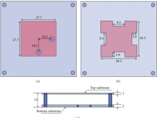
27.7 27.7 10.5 10.5 (a) 28.5 28.5 9.5 9.5 3.9 3.9 (b) 2 1 12 Top substrate Bottom substrate (c)
Figure 2: Configurations of the stacked microstrip antenna. (a) Top view of bottom layer. (b) Top view of top layer. (c) Side view (all units are in mm).
few harmonics should be taken into account to ensure the sideband level suppression is conducted.
3. MOPSO Algorithm
3.1. Terminologies of Multiobjective Optimizations. Without
loss of generality, the following minimization problem is to be considered: Minimize 𝑓 ( ⃗𝑥) = {𝑓⃗ 1( ⃗𝑥) , 𝑓2( ⃗𝑥) , . . . , 𝑓𝑀( ⃗𝑥) , 𝑚 = 1, 2, . . . , 𝑀} , subject to constraints 𝑔𝑖( ⃗𝑥) ≤ 0; 𝑖 = 1, 2, . . . , 𝑝 ℎ𝑖( ⃗𝑥) = 0; 𝑖 = 1, 2, . . . , 𝑞, (9) where ⃗𝑥 = {𝑥𝑖, 𝑖 = 1, 2, . . . , 𝐷}is a vector of decision variables. These constraints define the feasible region, and any vector in the feasible region is called a feasible solution.
In multiobjective optimal problems, the following two terminologies are often used.
Dominance Relations.The definitions of dominance relations
between two vectors (or individuals of the population) are given in [21]. The weak dominance relation (⪯) between ⃗𝑥1 and ⃗𝑥2is defined as:
⃗𝑥
1 weak dominates ⃗𝑥2 ⃗𝑥1⪯ ⃗𝑥2 iff∀𝑖 : 𝑓𝑖( ⃗𝑥1) ≤ 𝑓𝑖( ⃗𝑥2)
(10)
while the dominance relation (≺) is defined as
⃗𝑥
1 dominates ⃗𝑥2 ⃗𝑥1≺ ⃗𝑥2
iff ⃗𝑥1⪯ ⃗𝑥2∧ ∃𝑖 : 𝑓𝑖( ⃗𝑥1) < 𝑓𝑖( ⃗𝑥2) . (11) The dominance relationship can be extended to take into consideration constraint values besides objective val-ues; the relation constraint-dominance (≺𝑐) is defined as:
⃗𝑥
1 constraint-dominates ⃗𝑥2 ⃗𝑥1≺𝑐 ⃗𝑥2, if any of the following
conditions is true.
(1) ⃗𝑥1belongs to the feasible space and ⃗𝑥2does not. (2) ⃗𝑥1and ⃗𝑥2are both infeasible and ⃗𝑥1dominates ⃗𝑥2in
constraint function space.
(3) ⃗𝑥1and ⃗𝑥2are feasible and ⃗𝑥1dominates ⃗𝑥2in objective function space.
Pareto Optimal (Solution, or Front). The strongly and weakly
nondominated solutions constitute the total Pareto front of a multiobjective optimization problem.
3.2. MOPSO Algorithm. Particle swarm optimization (PSO)
is a stochastic population-based multipoint search optimiza-tion technique developed by Eberhart and Kennedy in 1995 [22], inspired by the social behavior of bird flocking or fish schooling. In PSO, each particle has a position vector
⃗𝑥
𝑖 = (𝑥𝑖1, 𝑥𝑖2, . . . , 𝑥𝑖𝐷)in the 𝐷-dimensional search space
and moves through the problem space, with the moving velocity of each particle represented by a position vector
(a) (b)
Figure 3: Photograph of the fabricated antenna. (a) Top layer. (b) Bottom layer.
6 5 4 3 2 1 V SWR 2.8 2.9 3.0 3.1 3.2 3.3 3.4 3.5 3.6 Frequency (GHz) Measured results Simulated results
Figure 4: Simulated and measured VSWR for the antenna.
x y z ̂𝜑 ̂𝜃 𝜃-feed points 𝜑-feed points
Figure 5: The schematic diagram of the antennas positioned on the conical surface with the𝜃-feed points in thê𝜃-direction and the𝜑 -feed points in thê𝜑-direction.
Copolarized direction beam direction (𝜃d, 𝜑d) En𝜑 𝛼nE𝜃n𝜑 𝛽nE𝜑n𝜃 𝛽nE𝜑n𝜃 𝛾d En ̂𝜑 ̂𝜃 En𝜑 𝛼nE𝜃n𝜃
Sample point in main
Figure 6: A graphical representation of the relations between the desired polarization vector in the main beam direction and the various components of the radiated field.
−40 −35 −30 −25 −20 −15 −10 −45 −40 −35 −30 −25 −20 −15 −10 MSLL (dB) MS BL (dB) Solution A
Figure 7: Pareto front obtained by the proposed MOPSO for scan direction of(74∘, 0∘).
0 2040 60 80 100120140 160180 −80 −60 −40 −20 0 20 40 60 80 0 The co p o la ri za tio n pa tt er n (dB) −80 −70 −60 −50 −40 −30 −20 −10 0 𝜃(deg) 𝜑(deg) −20 −40 −60 −80 2040404040440404040440404040404040404040400000000000000000000000000066666666606666666666060666060606060606606060606606060660666000000 80 8 80 8 8 8 80 80 80 80 80 80 80 8 80 80 80 80 80 80 80 80 80 800 80 800 80 80 80000000000100101010010100100101010100100100100100101001001001100101100100000000000000000000000000000000001201201201201201201212012012012121201201201201201201202020202020202202020000 140 1 1 1 1 1 1 1 1 1 1 1 1 1 10016 80 −60 −6 −60 −60 −60 −60 −60 −6 −606 −60 −60 −60 −606 −6 −60 −660 −6 −6060606066 −6 −6 −6 −660 −6 − −6 −6 −6 −60 −6 −6 − −6 −6 − −6 − − − − − − − − − − − − − − −66 −40 −4 −4 − − − −4 − −4 −4 − − − − −4 −4 −44444 −202202020202022202022020220202020202020000000000000 −202202020000 −20 −20220200000 −20 −20 −20 −20 −20 − −20 − −20 −202000 −20 −20 −20 − −20 −20 − − −20 − −2020202020000 0 0 0 0 0 0 0 0 0 0 0 0 0 0 0 0 0 0 0 0 0 0 0 0 0 0 0 0 20 40 4 4 4 4 4 4 4 4 40 40 60 0 𝜃 𝜃 𝜃 𝜃(((de(de((de(((((((((((ddededddedededededdeddeddeddededdddededededdedddddddddddededeeeg)gg)g)ggg)gg)g))))))))))))))))))
𝜑 𝜑 𝜑 𝜑 𝜑 𝜑 𝜑 𝜑 𝜑 𝜑 𝜑 𝜑 𝜑 𝜑 𝜑 𝜑 𝜑 𝜑 𝜑 𝜑 𝜑 𝜑 𝜑 𝜑 𝜑 𝜑 𝜑(de d (d (d (d (de (d (de (d (de ( (d (d (de (d (de (de (de ( (d (d (de (dde (d (d (de (dde eg)
(a) Copolarization pattern
0 2040 60 80 100120 140160 180 −80 −60 −40 −200 20 40 60 80 −70 −60 −50 −40 −30 −20 −10 0 The cr oss-p o la riza tio n pa tt er n (dB) −160 −140 −120 −100 −80 −60 −40 𝜃(deg) 𝜑(deg) 20 4060 80 10012000000000000000000000000000000000 140 0 0 16 80 −6066666666666666666666666666666066666066606666660 −40 −200 20 40 4 400 4 4 4 4000000000000 60 0 𝜃(deg)g)g)g)g)g)g)g)g)g)g)g)g)g)gg)g)g)g)g)gg)g)g)))))))))))) 𝜑(de g) (b) Cross-polarization pattern
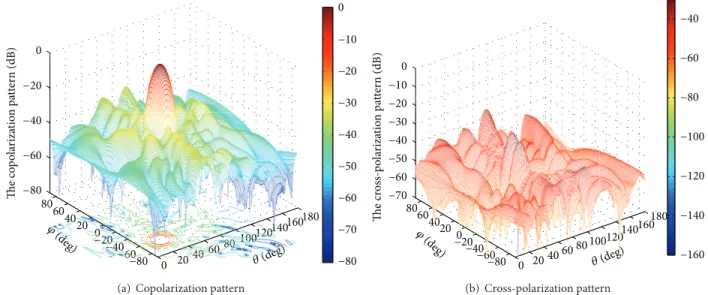
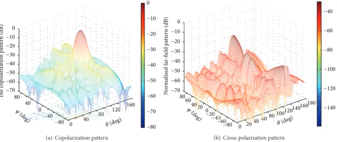
Figure 8: 3D radiation pattern of the conical conformal array for scan direction of(74∘, 0∘)for solution A inFigure 7.
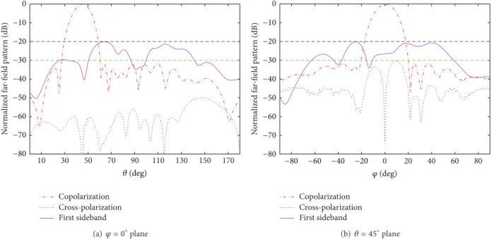
10 30 50 70 90 110 130 150 170 0 N o rm alized fa r-field p at ter n (dB) Copolarization Cross-polarization First sideband 𝜃(deg) −10 −20 −30 −40 −50 −60 −70 −80 (a)𝜑 = 0∘plane 0 20 40 60 80 0 N o rm alized fa r-field p at ter n (dB) 𝜑(deg) −10 −20 −30 −40 −50 −60 −70 −80 −20 −40 −60 −80 Copolarization Cross-polarization First sideband (b) 𝜃 = 74∘plane
Figure 9: Sectional views in the elevation and azimuth planes for scan direction of(74∘, 0∘)for solution A inFigure 7.
⃗
V𝑖 = (V𝑖1,V𝑖2, . . . ,V𝑖𝐷). Each particle keeps track of its own best position𝑝best𝑖 = (𝑝best𝑖1, 𝑝best𝑖2, . . . , 𝑝best𝑖𝐷)and the best position among all the particles obtained so far in the population𝑔best = (𝑔best1, 𝑔best2, . . . , 𝑔best𝐷), which are given by
V𝜏+1𝑖𝑑 = 𝑤V𝜏𝑖𝑑+ 𝑐1𝑟1𝑑(𝑝best𝜏𝑖𝑑− 𝑥𝜏𝑖𝑑) + 𝑐2𝑟2𝑑(𝑔best𝜏𝑑− 𝑥𝜏𝑖𝑑) , (12)
𝑥𝜏+1𝑖𝑑 = 𝑥𝑖𝑑𝜏 +V𝜏+1𝑖𝑑 , (13) where 𝑐1 and 𝑐2 are acceleration constants and𝑟1𝑑 and 𝑟2𝑑 are uniformly distributed random numbers in[0, 1].𝑤is the inertia weight factor.
Since PSO cannot be directly applied to multiobjective optimization, there are two major issues to be considered when extending PSO to multiobjective optimization. The first one is how to select the global and local best particles (leaders) to guide the search of a particle. The second one is how to maintain good points found so far. The algorithm based on the repository of particles [23] and mutation operator in multiobjective particles swarm optimization (MOPSO) is adopted in this paper. The steps of the MOPSO are briefly given in the following.
Step 1. Initialize the population: given the population scale
𝑃, randomly generate the position of each particle𝑃[𝑖]and initialize the velocity of each particleV[𝑖]to 0.
Step 3. Store the positions of the particles which represent nondominated vectors in the repository Rep.
Step 4. Generate hypercubes of the search space and locate
the particles using these hypercubes as a coordinate system.
Step 5. Initialize the memory of each particle, which serves
as a guide to travel through the search space.
Step 6. Compare current loop iteration to the maximum
iterations to decide whether to continue to iterate again.
Step 6.1. Compute the speed of each particle as follows:
V𝜏+1𝑖𝑑 = 𝑤V𝜏𝑖𝑑+ 𝑐1𝑟1𝑑(𝑝best𝜏𝑖𝑑− 𝑥𝜏𝑖𝑑) + 𝑐2𝑟2𝑑(Rep[ℎ]𝜏𝑑− 𝑥𝜏𝑖𝑑) . (14) Different from (12), its own best position in (14) is judged by the dominance principle and the global best is replaced by Rep taken from the repository.
Step 6.2. Compute the new positions of the particles and
maintain the particles within the search space.
Step 6.3. Update the contents of Rep and the geographical
representation of the particles within the hypercubes.
Step 6.4. Update particles’ own best position𝑝best𝑖.
Step 7. Repeat the above Steps2to6until a stopping criterion
is stratified. In this paper, the MOPSO ends if the algorithm reaches the maximum amount of iterations or the maximum execution time.
4. Numerical Results
4.1. Array Element Antenna Design. As microstrip patch
antennas have the advantages of light weight, low profile, and low cost, they are extensively utilized as the array element. With a center frequency of 3.2 GHz, a compact dual-fed stacked microstrip antenna is designed as the element of the conformal conical array. Its geometry is given in Figure 2, which is fabricated on two layers with relative permittivity of 2.65. This antenna utilizes a one-order quasi-Minkowski fractal patch on the top substrate to reduce the patch size, which also reduces the coupling between adjacent elements. The antenna is fed by standard SMA coaxial connectors from the bottom.Figure 3shows the photograph of the fabricated antenna.
Figure 4displays the measured and simulated impedance
bandwidth for the antenna. The measured impedance band-width (VSWR≤2) by Agilent N5230A network analyzer is from 3.0 to 3.61 GHz (18.46%). There is a good agreement between simulated and measured results. Therefore, the designed antenna can fully satisfy the demanded require-ments.
For conformal arrays, to determine the total radiation pattern produced at a far-field point, it is more convenient
−30 −35 −40 −45 −50 −55 Harmonic mode,q Sideba nd le ve l (dB) 0 5 10 15 20 25 30
Figure 10: The maximum sideband levels of the first 30 positive harmonics for scan direction of(74∘, 0∘)for solution A inFigure 7.
to consider the field of individual elements in their own coordinate systems firstly and then transform the field back to the global coordinate system [24].
4.2. Pattern Synthesis. Since polarization plays a very
impor-tant role in conformal phased arrays, the polarization radia-tion pattern is investigated in this paper. To reduce the cross-polarization of the conical array, the technique based on combining the weighted individual feeding ports of the patch antennas before beamforming is employed in this paper [25]. As shown inFigure 5, each antenna is fed using dual feeds. For the𝑛th radiator, the𝜃-feed point will excite two radiated fields, that is, a copolarized field 𝐸𝑛𝜃𝜃 , in the ̂𝜃-direction and a cross-polarized component𝐸𝜃𝑛𝜑. Similarly, the𝜑-feed point will result in a copolarized radiated field𝐸𝜑𝑛𝜑in the ̂𝜑 -direction and a cross-polarized component𝐸𝜑𝑛𝜃. Besides, the polarization angle (𝛾𝑑) for linear polarization is defined as the angle between the ̂𝜃-unit vector and the unit vector in the direction of the desired polarization at the field point in the direction of the main beam, as shown inFigure 6.
For the𝑛th element, the unit vector of the desired polar-ization is a linear combination of the𝜃- and𝜑-components of the radiated field in the direction of the main beam as follows:
𝐸𝑛(𝜃𝑑, 𝜑𝑑)sin𝛾𝑑= 𝛼𝑛𝐸𝑛𝜑𝜃 (𝜃𝑑, 𝜑𝑑) + 𝛽𝑛𝐸𝜑𝑛𝜑(𝜃𝑑, 𝜑𝑑) ,
𝐸𝑛(𝜃𝑑, 𝜑𝑑)cos𝛾𝑑= 𝛼𝑛𝐸𝑛𝜃𝜃 (𝜃𝑑, 𝜑𝑑) + 𝛽𝑛𝐸𝜑𝑛𝜃(𝜃𝑑, 𝜑𝑑) , (15)
where 𝐸𝑛(𝜃𝑑, 𝜑𝑑) is the desired polarization from the 𝑛th radiator in the direction of the main beam.𝐸𝜃𝑛𝜑(𝜃𝑑, 𝜑𝑑)and
𝐸𝜑
𝑛𝜑(𝜃𝑑, 𝜑𝑑)are the𝜑-components of the radiated field from
𝜃- and𝜑-feed point of the𝑛th radiator, respectively. Whereas,
𝐸𝜃
𝑛𝜃(𝜃𝑑, 𝜑𝑑)and𝐸𝜑𝑛𝜃(𝜃𝑑, 𝜑𝑑)are the𝜃-components from𝜃- and
𝜑-feed point of the𝑛th radiator, respectively.𝛼𝑛and𝛽𝑛 are, respectively, the weights for the𝜃- and𝜑-feed point of the𝑛th
1 2 3 4 5 6 7 8 910 11 1213 1 2 3 45 67 8 910 11 12 0 0.5 1 N M Sw it ch -o n d ura tio n
(a) Theta feed point
1 2 3 4 5 6 7 8 9 101112 13 12 3 45 67 8 9 10 1112 0 0.2 0.4 0.6 0.8 N M Sw it ch -o n d ura tio n
(b) Phi feed point
Figure 11: Optimized switch-on durations in the theta feed point and phi feed point for scan direction of(74∘, 0∘)for solution A inFigure 7.
0 40 80 120 160 200 −100 −60 −200 20 60 100 −70 −60 −50 −40 −30 −20 −10 0 The co p o la riza tio n pa tt er n (dB) −80 −70 −60 −50 −40 −30 −20 −10 0 𝜃(deg) 𝜑(deg) 4 40 4 4 4 4 4 4 40 4000 4 4 4 4 4 40 40 40 40 40 40 40 40 4 400 88888888880880880808080808088080808 120222222222222222222222222222222222222 1 −60606060 −6 −66060606060 −6 −6 −60 −6 −66060606060 −60 −60 −6 −6000 −6066066000 −6600 −606666666666600 −20 −202000 −2020 −20020202200 20 60 𝜃(de(d((d(d(d(d(d(((d(d(dg) 𝜑(de e e eg)g)g)g)g)g)g)g)g)g)g) ) ) g g))) g)) g g) g) g g) g g g g g g g) g) g g g g)
(a) Copolarization pattern
0 2040 60 80100 120140160 180 −80 −60 −40 −20 0 20 40 60 80 −70 −60 −50 −40 −30 −20 −10 0 The cr oss-p o la riza tio n pa tt er n (dB) −160 −140 −120 −100 −80 −60 −40 𝜃(deg) 𝜑(deg) 20 406060666666060660606666066066660660606660660606066666666606666660660606660660606066606060000000 80 8 80 80 80 80 80000 80 800 80 8000000 80 80 800 80 8000 80000 80 800 80 8 800 800000000000 80 800000000000 8 11110110010011001011111001001100100100101001110100111110101100110010010100101010101111100111101001101100000000000000000000000000000000000000000000000000000 1 120 120 1 1 1200 1 1 120 1 1 1 1 1 1 1 1 1 1 1 1 1 1 1 1 1 1 1 1 0 0 1414014141114144444444444444444444 16 80 −606 −6 − −6 − −6 − −66 −6 − −66 −66 −66 − −66 −666 −66 −6666666666 −6 − −6666666 −400000000000000000000000000000000000000000000 −20 0 20 40 60 0 𝜃(deg) 𝜑(deg) (b) Cross-polarization pattern
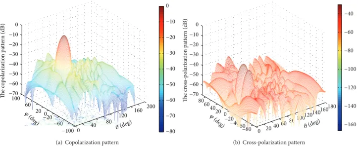
Figure 12: 3D radiation pattern of the conical conformal array for scan direction of(45∘, 0∘)for solution A inFigure 7.
radiator to achieve the required polarization in the direction of the main beam. From (15) we can derive that
tan𝛾𝑑=𝛼𝑛𝐸 𝜃 𝑛𝜑(𝜃𝑑, 𝜑𝑑) + 𝛽𝑛𝐸𝜑𝑛𝜑(𝜃𝑑, 𝜑𝑑) 𝛼𝑛𝐸𝜃 𝑛𝜃(𝜃𝑑, 𝜑𝑑) + 𝛽𝑛𝐸𝜑𝑛𝜃(𝜃𝑑, 𝜑𝑑) . (16)
From (16), the ratio of the excitation amplitude between the two feed ports can be written as
𝛽𝑛 𝛼𝑛 =
tan𝛾𝑑𝐸𝜃𝑛𝜃(𝜃𝑑, 𝜑𝑑) − 𝐸𝜃𝑛𝜑(𝜃𝑑, 𝜑𝑑)
𝐸𝑛𝜑𝜑 (𝜃𝑑, 𝜑𝑑) −tan𝛾𝑑𝐸𝜑𝑛𝜃(𝜃𝑑, 𝜑𝑑)
. (17)
Thus, before the synthesis of the radiation patterns, the excitation relation between the two feed ports can be
determined, which can be used to effectively reduce half of the optimization variables.
The arrays considered here are fed with a uniform static excitation (|𝐼𝑛| = 1), a target of which is always desired in practice. For conformal arrays, it is common to select the excitation phase to focus the beam in the desired direction. With the phase excitation calculated by (2), the specified scan angle can be guaranteed. Only the pulse durations are considered in the numerical simulation later. In this paper, a
12 × 13conical conformal phased array is investigated; that is, the array consists of 156 elements. Now considering that the optimization for the pulse durations of each element on the conical phased array may be a prohibitive task in practical engineering, then, a previously proposed modified Bernstein
10 30 50 70 90 110 130 150 170 N o rm alized fa r-field p at ter n (dB) 𝜃(deg) −20 −30 −40 −50 −60 −70 −80 Copolarization Cross-polarization First sideband (a)𝜑 = 0∘plane 0 20 40 60 80 N o rm alized fa r-field p at ter n (dB) 𝜑(deg) −20 −30 −40 −50 −60 −70 −80 −20 −40 −60 −80 Copolarization Cross-polarization First sideband (b)𝜃 = 45∘plane
Figure 13: Sectional views in the elevation and azimuth planes for scan direction of(45∘, 0∘)for solution A inFigure 7. polynomial for arc arrays [5] is extended to 3D case to be used.
The modified Bernstein polynomial is defined as
𝐹 (𝑈) = { { { { { { { { { { { { { { { { { 𝐵1+ 1 − 𝐵1 𝐴𝑁0𝐴(1 − 𝐴)𝑁0(1−𝐴)𝑈 𝑁0𝐴(1 − 𝑈)𝑁0(1−𝐴), 0 ≤ 𝑈 ≤ 𝐴 𝐵2+ 1 − 𝐵2 𝐴𝑁1𝐴(1 − 𝐴)𝑁1(1−𝐴)𝑈 𝑁1𝐴(1 − 𝑈)𝑁1(1−𝐴), 𝐴 ≤ 𝑈 ≤ 1, (18) where 𝐵1, 𝐵2, 𝑀1, 𝑀2, and 𝐴are parameters in the poly-nomial. By using the modified Bernstein polynomial, in our pattern synthesis example only five variables need to be optimized of each concentric ring. The differences among the maximum amplitude of each row are also obtained by a modified Bernstein polynomial. That is to say, for a spherical conformal array constituting of𝑀concentric circular arrays, the total number of variables to be optimized can be reduced to5 × (𝑀 + 1), which can significantly alleviate the burden of the algorithm in the optimization process. For the conical conformal array consisting of 12 rows, the total number of variables to be optimized is reduced from 12×13 to 5×(12 + 1); that is, the optimization variables can be reduced by 58.3%. In this paper, the third definition of Ludwig is used to define the copolarization𝐸coand the cross-polarization𝐸cross [26] as follows:
𝐸co= 𝐸𝜃cos𝜑 − 𝐸𝜑sin𝜑,
𝐸cross= 𝐸𝜃sin𝜑 + 𝐸𝜑cos𝜑.
(19) To illustrate the effectiveness of the proposed mechanism, the three-dimensional (3D) radiation patterns of the array are synthesized in three scan angles:(74∘, 0∘),(45∘, 0∘), and
(105∘, 0∘). For this time-modulated conformal array, we focus
on achieving low sidelobe level and low sideband level simultaneously as follows:
min FF( ⃗𝑥) = {SLL( ⃗𝑥) ,SBL( ⃗𝑥)} . (20) Behavior of the MOPSO on the considered synthesis problem has been investigated. Simulation results show that to ensure the convergence of the optimization process, parameters in (14) should satisfy0.5(𝑐1 + 𝑐2) < 1.5(1 + 𝑤) condition and in such case the population mean converges to the desired solution set. Otherwise, the algorithm may fail to converge to the desired solution set. Thus, in the numerical experiments, the inertia weight factor𝑤is chosen to be 0.4, the acceleration constants𝑐1 = 𝑐2 = 1. The population size is set to 100, the repository size𝑟𝑝 = 100, the mutation rate
𝑚𝑢 = 0.5, and the maximum number of generations is set to 2000. The proposed approach runs on an I7-2620 2.7 GHz CPU with 4 GB memory. The simulation times for different scan angles are roughly the same, which is about 22.32 minutes. The distribution of the Pareto front (PF) achieved by the MOPSO for scan direction of (74∘, 0∘) is shown in
Figure 7. The coordinate values of the axes represent the
maximum SLL (MSLL) at𝑓0and the maximum SBL (MSBL). Each point of the Pareto front represents a feasible design case, which can provide great freedom to the designers, as compared with the single-objective optimization techniques. To further validate the effectiveness of the proposed method, the normalized radiation patterns for one of the solutions, solution A (inFigure 7), are plotted, as presented inFigure 8. The copolarization and cross-polarization patterns and the first sideband cuts through the main beam at𝜑 = 0∘ and
𝜃 = 74∘ are illustrated inFigure 9. From those simulation
results, it can be seen that the main beam points in the desired direction with sidelobe levels are below−30 dB and
1 2 3 4 5 6 7 8 9 1011 12 13 12 3 4 5 67 8 9 10 1112 0 0.5 1 N M Sw it ch -o n d ura tio n
(a) Theta feed point
1 2 3 4 5 6 7 8 9 10 11 1213 12 3 45 67 8 9 1011 12 0 0.2 0.4 0.6 0.8 N M Sw it ch -o n d ura tio n
(b) Phi feed point
Figure 14: Optimized switch-on durations in the theta feed point and phi feed point for scan direction of(45∘, 0∘)for solution A inFigure 7.
0 40 80 120 160 −80 −40 0 40 80 −70 −60 −50 −40 −30 −20 −10 0 The co p o la riza tio n pa tt er n (dB) −80 −70 −60 −50 −40 −30 −20 −10 0 𝜃(deg) 𝜑(deg) 40 40 4 40 40000000 40000000 4 4000 4 4000 4 4 40000 4 4 40000 4 4000 4 4000 400 88888888888880880888888808 1200000000000000000000000000 16 80 80 80 −40 −40 −40 −40 −4 −40 −40 −40 −40 −440 −40 −40 −40 −40 −40 −4 −4 −4 −40 −40 −40 −40 − −4 −4 −40 −40404 −44440 −4 −4 −4440404444404000 0 40 0 deeeeeg)gg 𝜑(de de de de de de de de deeeeeeeeeeeeeeee g) g) g) g) g) g) g) g) g) g) g) g) g) g) g)) g) g) g) g) g) g) g g g g g g g g g) g)
(a) Copolarization pattern
0 2040 60 80 100120140 160180 −80 −60 −40 −20 0 20 40 60 80 −70 −60 −50 −40 −30 −20 −10 0 N o rm alized fa r-field pa tt er n (dB) −140 −120 −100 −80 −60 −40 2 2 20 2 20 200 200 2 2 2 20 2 2 20 2 20 20000444444444444444444444444444444404444444444 6666666666666666666666666666666666066666666666666666666666666666 8000000000000000000000000000000000000000000001111111111111111111111111111110011111111111111111 1111111111111111111111111111201111 14016 80 −60 − − − − −40000000000000000000000000000000000 −20 0 2 2 2 2 2 2 2 20 2 2 2 2 2 2 2 2 2 2 2 2 2 2 2 2 2 2 2 2 2 2 2 2 2 2 2 2 2 2 2 2 2 2 2 2 2 2 2 2 2 2 2 2 2 2 2 2 2 2 2 2 2 2 2 2 2 2 2 40000000000000000000000000000000000000000000 60 0 𝜃(deg) 𝜑(deg) (b) Cross-polarization pattern
Figure 15: 3D radiation pattern of the conical conformal array for scan direction of(105∘, 0∘)for solution A inFigure 7.
the cross-polarization pattern for the array are also below
−30 dB. Furthermore, the MSBL for the first sidebands is
−20.08 dB, which can also be seen from Figures8and9. In order to prove the suppression of SBL, the maximum levels of first 30 harmonics in this direction are provided inFigure 10. For limited space, the figures corresponding to the other two scan angles are not provided because their results are similar to that inFigure 10.Figure 11provides the optimized pulse duration sequences for the dual-fed stacked microstrip elements in theta feed point and phi feed point.
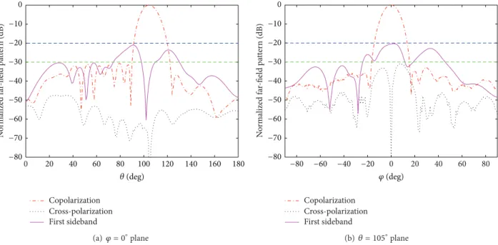
Due to the similar distributions of the Pareto front (PF) for scan directions of(45∘, 0∘)and(105∘, 0∘)as inFigure 7, they are not presented. Also, one of the solutions for these two scan directions chosen from the Pareto front is plotted. The 3D radiation patterns for these two scan angles are presented
in Figures12and 15, respectively. The corresponding copo-larization and cross-pocopo-larization patterns and first sideband cuts through the main beams are illustrated in Figures13and 16, respectively. From the figures, we can also discover that sidelobe levels are all below−30 dB and the cross-polarization patterns also below −30 dB. The required pulse duration sequences for the dual-fed stacked microstrip elements in theta feed point and phi feed point for these two scan angles are shown in Figures14and17, respectively.
5. Conclusion
This paper has presented time-modulated conformal phased array synthesis optimization by using the multiobjective particle swarm optimization. Conflicting specifications such
0 N o rm alized fa r-field p at ter n (dB) 𝜃(deg) −20 −30 −40 −50 −60 −70 −80 Copolarization Cross-polarization First sideband 20 40 60 80 100 120 140 160 180 (a)𝜑 = 0∘plane 0 20 40 60 80 N o rm alized fa r-field p at ter n (dB) 𝜑(deg) −20 −30 −40 −50 −60 −70 −80 −20 −40 −60 −80 Copolarization Cross-polarization First sideband (b)𝜃 = 105∘plane
Figure 16: Sectional views in the elevation and azimuth planes for scan direction of(105∘, 0∘)for solution A inFigure 7.
1 2 3 4 5 6 7 8 9 10 11 1213 1 23 4 5 67 89 10 11 12 0 0.5 1 N M Sw it ch -o n d u ra tio n
(a) Theta feed point
1 2 3 4 5 6 7 8 9 1011 1213 1 2 3 4 5 6 7 8 910 1112 0 0.2 0.4 0.6 0.8 N M Sw it ch -o n d u ra tio n
(b) Phi feed point
Figure 17: Optimized switch-on durations in the theta feed point and phi feed point for scan direction of(105∘, 0∘)for solution A inFigure 7.
as the peak SLL and SBL have been optimized simultaneously. Additionally, the modified Bernstein polynomial is extended to 3D case in synthesizing conformal arrays in order to greatly reduce the optimization variables. Dual fed patch antennas are designed as the radiating elements to achieve low cross-polarization level during the beam scanning. The proposed algorithm has been successfully applied to design a12 × 13 -element conical conformal microstrip phased array, which can provide great freedom to the designers as compared with the single-objective optimization techniques. The numerical results reveal the promising characteristics of the mechanism in synthesizing time-modulated conformal arrays.
Conflict of Interests
The authors declare that there is no conflict of interests regarding to the publication of this paper.
Acknowledgments
The authors would like to thank the financial support from the Natural Science Foundation of China (no. 61101069 and no. 61201135) and the Fundamental Research Funds for the Central Universities (no. K5051302022 and no. K7214569601).
References
[1] L. Josefsson and P. Persson,Conformal Array Antenna Theory and Design, John Wiley & Sons, New York, NY, USA, 2006. [2] K. Wincza, S. Gruszczynski, and K. Sachse, “Conformal
four-beam antenna arrays with reduced sidelobes,”Electronics Let-ters, vol. 44, no. 3, pp. 174–175, 2008.
[3] Y. Y. Bai, S. Xiao, C. Liu, and B. Z. Wang, “A hybrid IWO/PSO algorithm for pattern synthesis of conformal phased arrays,” IEEE Transactions on Antennas and Propagation, vol. 61, no. 4, pp. 2328–2332, 2013.
[4] O. M. Bucci, A. Capozzoli, and G. D’Elia, “Power pattern synthesis of reconfigurable conformal arrays with near-field constraints,”IEEE Transactions on Antennas and Propagation, vol. 52, no. 1, pp. 132–141, 2004.
[5] D. W. Boeringer and D. H. Werner, “Efficiency-constrained particle swarm optimization of a modified Bernstein polyno-mial for conformal array excitation amplitude synthesis,”IEEE Transactions on Antennas and Propagation, vol. 53, no. 8, pp. 2662–2673, 2005.
[6] L. I. Vaskelainen, “Constrained least-squares optimization in conformal array antenna synthesis,” IEEE Transactions on Antennas and Propagation, vol. 55, no. 3, pp. 859–867, 2007. [7] B. Fuchs, “Shaped beam synthesis of arbitrary arrays via
linear programming,”IEEE Antennas and Wireless Propagation Letters, vol. 8, pp. 481–484, 2010.
[8] K. M. Tsui and S. C. Chan, “Pattern synthesis of narrowband conformal arrays using iterative second-order cone program-ming,”IEEE Transactions on Antennas and Propagation, vol. 58, no. 6, pp. 1959–1970, 2010.
[9] H. E. Shanks and R. W. Bickmore, “Four-dimensional electro-magnetic radiators,”Canadian Journal of Physics, vol. 37, no. 3, pp. 263–275, 1959.
[10] L. Poli, P. Rocca, L. Manica, and A. Massa, “Handling sideband radiations in time-modulated arrays through particle swarm optimization,”IEEE Transactions on Antennas and Propagation, vol. 58, no. 4, pp. 1408–1411, 2010.
[11] J. Fondevila, J. C. Br´egains, F. Ares, and E. Moreno, “Optimizing uniformly excited linear arrays through time modulation,”IEEE Antennas and Wireless Propagation Letters, vol. 3, no. 1, pp. 298– 301, 2004.
[12] S. W. Yang, Y. B. Gan, and A. Y. Qing, “Sideband suppression in time-modulated linear arrays by the differential evolution algorithm,”IEEE Antennas and Wireless Propagation Letters, vol. 1, pp. 173–175, 2002.
[13] S. K. Mandal, R. Ghatak, and G. K. Mahanti, “Minimization of side lobe level and side band radiation of a uniformly excited time modulated linear antenna array by using artificial bee colony algorithm,” inProceedings of the IEEE Symposium on Industrial Electronics and Applications (ISIEA ’11), pp. 247–250, September 2011.
[14] Q. Zhu, S. Yang, R. Yao, and Z. Nie, “Gain improvement in time-modulated linear arrays using SPDT switches,”IEEE Antennas and Wireless Propagation Letters, vol. 11, pp. 994–997, 2012. [15] Y. Wang and A. Tennant, “Time-modulated reflector array,”
Electronics Letters, vol. 48, no. 16, pp. 972–974, 2012.
[16] E. T. Bekele, L. Poli, P. Rocca, M. DUrso, and A. Massa, “Pulse-shaping strategy for time modulated arrays—analysis and design,”IEEE Transactions on Antennas and Propagation, vol. 61, no. 7, pp. 3525–3537, 2013.
[17] E. Aksoy and E. Afacan, “Calculation of sideband power radia-tion in time-modulated arrays with asymmetrically posiradia-tioned
pulses,”IEEE Antennas and Wireless Propagation Letters, vol. 11, pp. 133–136, 2012.
[18] A. Tennant, “Experimental two-element time-modulated direc-tion finding array,”IEEE Transactions on Antennas and Propa-gation, vol. 58, no. 3, pp. 986–988, 2010.
[19] G. Li, S. Yang, and Z. Nie, “Direction of arrival estimation in time modulated linear arrays with unidirectional phase center motion,”IEEE Transactions on Antennas and Propagation, vol. 58, no. 4, pp. 1105–1111, 2010.
[20] E. Aksoy and E. Afacan, “An inequality for the calculation of relative maximum sideband level in time-modulated linear and planar arrays,”IEEE Transactions on Antennas and Propagation, vol. PP, no. 99, 2014.
[21] K. Deb,Multiobjective Evolutionary Algorithm, John Wiley & Sons, Chichester, UK, 2001.
[22] R. Eberhart and J. Kennedy, “New optimizer using particle swarm theory,” inProceedings of the 6th International Sympo-sium on Micro Machine and Human Science, pp. 39–43, October 1995.
[23] C. A. C. Coello, G. T. Pulido, and M. S. Lechuga, “Handling multiple objectives with particle swarm optimization,” IEEE Transactions on Evolutionary Computation, vol. 8, no. 3, pp. 256–279, 2004.
[24] H. A. Burger, “Use of euler-rotation angles for generating antenna pattern,”IEEE Antennas and Propagationg Magazine, vol. 37, no. 2, pp. 56–63, 1995.
[25] C. Dohmen, J. W. Odendaal, and J. Joubert, “Synthesis of confor-mal arrays with optimized polarization,”IEEE Transactions on Antennas and Propagation, vol. 55, no. 10, pp. 2922–2925, 2007. [26] A. C. Ludwig, “The definition of cross polarization,” IEEE Transactions on Antennas and Propagation, vol. AP-21, no. 1, pp. 116–119, 1973.
International Journal of
Aerospace
Engineering
Hindawi Publishing Corporationhttp://www.hindawi.com Volume 2014
Robotics
Journal ofHindawi Publishing Corporation
http://www.hindawi.com Volume 2014
Hindawi Publishing Corporation
http://www.hindawi.com Volume 2014 Active and Passive Electronic Components
Control Science and Engineering Journal of
Hindawi Publishing Corporation
http://www.hindawi.com Volume 2014 Hindawi Publishing Corporation
http://www.hindawi.com Volume 2014 Hindawi Publishing Corporation
http://www.hindawi.com Journal of
Engineering
Volume 2014Submit your manuscripts at
http://www.hindawi.com
VLSI Design
Hindawi Publishing Corporation
http://www.hindawi.com Volume 2014
Hindawi Publishing Corporation
http://www.hindawi.com Volume 2014 Shock and Vibration Hindawi Publishing Corporation
http://www.hindawi.com Volume 2014
Civil Engineering
Advances inAcoustics and VibrationAdvances in Hindawi Publishing Corporation
http://www.hindawi.com Volume 2014 Hindawi Publishing Corporation
http://www.hindawi.com Volume 2014 Electrical and Computer Engineering
Journal of
Advances in OptoElectronics
Hindawi Publishing Corporation
http://www.hindawi.com Volume 2014
The Scientific
World Journal
Hindawi Publishing Corporationhttp://www.hindawi.com Volume 2014
Sensors
Journal of Hindawi Publishing Corporationhttp://www.hindawi.com Volume 2014
Modelling & Simulation in Engineering Hindawi Publishing Corporation
http://www.hindawi.com Volume 2014
Hindawi Publishing Corporation
http://www.hindawi.com Volume 2014 Chemical Engineering
International Journal of Antennas and Propagation International Journal of
Hindawi Publishing Corporation
http://www.hindawi.com Volume 2014
Hindawi Publishing Corporation
http://www.hindawi.com Volume 2014 Navigation and Observation International Journal of
Hindawi Publishing Corporation
http://www.hindawi.com Volume 2014