Bounded-Degree Vertex Deletion Problem
Robert Ganian
1Algorithms and Complexity Group, TU Wien, Vienna, Austria
Fabian Klute
Algorithms and Complexity Group, TU Wien, Vienna, Austria
Sebastian Ordyniak
Algorithms and Complexity Group, TU Wien, Vienna, Austria Abstract
We study the parameterized complexity of the Bounded-Degree Vertex Deletion problem (BDD), where the aim is to find a maximum induced subgraph whose maximum degree is below a given degree bound. Our focus lies on parameters that measure the structural properties of the input instance. We first show that the problem is W[1]-hard parameterized by a wide range of fairly restrictive structural parameters such as the feedback vertex set number, pathwidth, treedepth, and even the size of a minimum vertex deletion set into graphs of pathwidth and treedepth at most three. We thereby resolve the main open question stated in Betzler, Bredereck, Niedermeier and Uhlmann (2012) concerning the complexity of BDD parameterized by the feedback vertex set number. On the positive side, we obtain fixed-parameter algorithms for the problem with respect to the decompositional parameter treecut width and a novel problem-specific parameter called the core fracture number.
2012 ACM Subject Classification Theory of computation→Graph algorithms analysis, Theory of computation→Parameterized complexity and exact algorithms
Keywords and phrases Bounded-degree Vertex Deletion, Feedback Vertex Set, Parameterized Algorithms, Treecut Width
Digital Object Identifier 10.4230/LIPIcs.STACS.2018.33
Funding This work was supported by the Austrian Science Fund (FWF), project P26696.
1
Introduction
This paper studies the Bounded-Degree Vertex Deletion problem (BDD): given an undirected graph G, a degree bound d, and a limit `, determine whether it is possible to delete at most `vertices fromGin order to obtain a graph of maximum degree at mostd. Aside from being a natural generalization of the classical Vertex Cover problem, BDD has found applications in areas such as computational biology [17] and is the dual problem of the so-called s-Plex Detectionproblem in social network analysis [30, 3, 31, 35].
It is not surprising that the complexity of BDD and several of its variants has been studied extensively by the theory community in the past years [5, 4, 7, 6, 11, 26, 34, 35]. Since the problem is NP-complete in general, it is natural to ask under which conditions does the problem become tractable. In this direction, theparameterized complexityparadigm [13, 33, 9] allows a more refined analysis of the problem’s complexity than classical complexity. In the
1 Robert Ganian is also affiliated with FI MU, Brno, Czech Republic.
© Robert Ganian, Fabian Klute, and Sebastian Ordyniak; licensed under Creative Commons License CC-BY
parameterized setting, we associate each instance with a numerical parameterkand are most often interested in the existence of afixed-parameter algorithm, i.e., an algorithm solving the problem in timef(k)· |V(G)|O(1)for some computable functionf. Parameterized problems admitting such an algorithm belong to the class FPT; on the other hand, parameterized problems that are hard for the complexity classW[1] orW[2] do not admit fixed-parameter algorithms (under standard complexity assumptions).
In general, there exist two notable approaches for selecting parameters: a parameter may either originate from the formulation of the problem itself (often called natural pa-rameters), or rather from the structure of the input graph (so-calledstructural parameters, most prominently represented by the decomposition-based parametertreewidth tw). The parameterized complexity of BDD has already been studied extensively through the lens of natural parameters (especiallyd and `). In particular, BDD is known to be FPT when parameterized byd+`[34, 17, 31],W[2]-hard when parameterized only by`[17], andNP -complete when parameterized only by d(as witnessed by the case of d = 0, i.e., Vertex Cover). The complexity of BDD is also fairly well understood when considering combina-tions of natural and structural parameters: it isFPTwhen parameterized bytw+ddue to Courcelle’s Theorem [8] and has been shown to beFPTwhen parameterized bytw+`[5].
Given the above, it is fairly surprising that the problem has remained fairly unexplored when viewed through the lens of structural parameters only, i.e., in the case where we impose no restrictions on the problem formulation itself but only on the structure of the graph. BDD was shown not to beFPTwhen parameterized by treewidth [5], complementing the previous
O(ntw+1) algorithm of Dessmark et al. [11]. The only structural parameter which is known to make the problem fixed-parameter tractable is the feedback edge set number, i.e., the minimum number of edges whose deletion results in a forest [5].
Contribution
The goal of this paper is to provide new insight into the complexity of BDD parameterized by the structure of the input graph. Our first main result shows that BDD is W[1]-hard parameterized by thefeedback vertex set number, i.e., the minimum number of vertices whose deletion results in a forest. This resolves the main open question in [5]. Interestingly, our result is significantly stronger since we show that hardness even applies in the case that the remaining parts, after deleting the feedback vertex set, are trees of height three. This rules out fixed-parameter algorithms w.r.t. most of the remaining “classical” decomposition-based structural parameters such aspathwidth andtreedepth [32] as well as w.r.t. thevertex deletion distance[19, 32] to bounded pathwidth, treedepth, and treewidth. On the way to our hardness result we show hardness for several multidimensional variants of the classical subset sum problem parameterized by the number of dimensions, which we believe are interesting on their own.
In light of the above, it is natural to ask whether there exist natural decomposition-based parameters for which BDD is fixed-parameter tractable. Our main algorithmic result answers this question affirmatively: we obtain a fixed-parameter algorithm utilizing the recently introduced structural parameter called treecut width. The importance of treecut width is that it plays a similar role with respect to the fundamental graph operation of immersion as the graph parametertreewidth plays with respect to the minor operation [36, 29]. Up to now, only a handful of problems are known to beFPTwhen parameterized by treecut width butW[1]-hard when parameterized by treewidth [20]. Furthermore, unlike previously known algorithms using treecut width, this is the first of its kind which does not use an Integer Linear Programming formulation but instead relies purely on combinatorial arguments.
Our second algorithmic result focuses on structural parameters which are not based on any particular decomposition of the graph, but instead measure the “vertex-deletion dis-tance” to a certain graph property. Such structural parameters have been successfully used in the past for a plethora of other difficult problems [19, 22, 27, 15, 14, 21]. In this context and taking into account the strong lower bounds obtained in Section 3, we introduce a struc-tural parameter which is specifically tailored to BDD and which we call the core fracture number. Roughly speaking, the core fracture numberk is the vertex deletion distance to a graph where each connected component only contains at mostk vertices which exceed the degree bound d. We show that computing the core fracture number isFPT which in turn gives rise to a fixed-parameter algorithm for BDD; the latter is achieved by identifying and formalizing a type-aggregation condition, allowing for an encoding of the problem into an Integer Linear Program with a controlled number of integer variables. This also resolves the question from [5] if BDD isFPTparametrized by vertex cover.
Finally, we exclude the existence of apolynomial kernel [13, 9] for BDD parameterized by the treecut width and core fracture number, and compare the two parameters in Section 5.
2
Preliminaries
2.1
Basic Notation
We use standard terminology for graph theory, see for instance [12]. All graphs except for those used to compute the torso-size in Subsection 2.3 are simple; the multigraphs used in Subsection 2.3 have loops, and each loop increases the degree of the vertex by 2.
Let Gbe a graph. We denote byV(G) andE(G) its vertex and edge set, respectively. For a vertexv ∈ V(G), let NG(v) ={y ∈V(G) :vy ∈E(G)}, NG[v] =NG(v)∪ {v}, and degG(v) denote its open neighborhood, closed neighborhood, and degree, respectively. For a subset X ⊆V(G), the (open) neighborhood NG(X) ofX is defined as Sx∈XN(x)\X. The setNG[X] refers to the closed neighborhood of X defined asNG(X)∪X. We refer to the setNG(V(G)\X) as∂G(X); this is the set of vertices in X which have a neighbor in
V(G)\X. We omit the lower indexG, ifGis clear from the context. For a vertex setA, we useG−Ato denote the graph obtained from Gby deleting all vertices inA. We use [i] to denote the set{0,1, . . . , i}. For completeness, we provide a formal definition of our problem of interest below.
Bounded-Degree Vertex Deletion (BDD)
Input: An undirected graphG= (V, E) and integers d≥0 and`≥0. Question: Is there a subsetV0⊆V with|V0| ≤
`whose removal fromGyields a graph in which each vertex has degree at mostd?
2.2
Parameterized Complexity
Aparameterized problemP is a subset of Σ∗×Nfor some finite alphabet Σ. LetL⊆Σ∗be a classical decision problem for a finite alphabet, and letpbe a non-negative integer-valued function defined on Σ∗. Then L parameterized by p denotes the parameterized problem
{(x, p(x))| x∈L} where x∈Σ∗. For a problem instance (x, k) ∈Σ∗×
N we call x the main part and k the parameter. A parameterized problem P is fixed-parameter tractable (FPT in short) if a given instance (x, k) can be solved in time O(f(k)·p(|x|)) wheref is an arbitrary computable function of k and pis a polynomial function; we call algorithms running in this timefixed-parameter algorithms. We refer the reader to [13] for more details on parameterized complexity.
Parameterized complexity classes are defined with respect tofpt-reducibility. A parame-terized problemP isfpt-reducibletoQif in timef(k)· |x|O(1), one can transform an instance (x, k) of P into an instance (x0, k0) of Q such that (x, k) ∈ P if and only if (x0, k0)∈ Q, and k0 ≤g(k), where f and g are computable functions depending only onk. Central to parameterized complexity is the following hierarchy of complexity classes, defined by the closure of canonical problems under fpt-reductions: FPT ⊆ W[1]⊆ W[2] ⊆ · · · ⊆ XP. All inclusions are believed to be strict. In particular,FPT6=W[1] under the Exponential Time Hypothesis [23].
The class W[1] is the analog of NP in parameterized complexity. A major goal in pa-rameterized complexity is to distinguish between papa-rameterized problems which are inFPT
and those which areW[1]-hard, i.e., those to which every problem inW[1] is fpt-reducible. There are many problems shown to be complete for W[1], or equivalently W[1]-complete, including theMulti-Colored Clique (MCC)problem [13].
2.3
Treecut Width
The notion of treecut decompositions was first proposed by Wollan [36], see also [29]. A family of subsetsX1, . . . , Xk ofX is anear-partitionofX if they are pairwise disjoint and
Sk
i=1Xi=X, allowing the possibility ofXi =∅.
IDefinition 1. Atreecut decompositionofGis a pair (T,X) which consists of a rooted tree
T and a near-partition X ={Xt ⊆V(G) :t ∈ V(T)} of V(G). A set in the familyX is called abagof the treecut decomposition.
For any node t of T other than the root r, let e(t) = ut be the unique edge incident tot on the path to r. Let Tu and Tt be the two connected components in T−e(t) which containuand t, respectively. Note that (S
q∈TuXq,
S
q∈TtXq) is a near-partition ofV(G),
and we usecut(t) to denote the set of edges with one endpoint in each part. We define the adhesionoft (adhT(t) oradh(t) in brief) as|cut(t)|; ift is the root, we setadhT(t) = 0 andcut(t) =∅.
The torso of a treecut decomposition (T,X) at a node t, written as Ht, is the graph obtained fromGas follows. IfT consists of a single nodet, then the torso of (T,X) att is
G. Otherwise letT1, . . . , T`be the connected components ofT−t. For eachi= 1, . . . , `, the vertex setZi⊆V(G) is defined as the set Sb∈V(Ti)Xb. The torsoHtatt is obtained from
Gbyconsolidatingeach vertex setZiinto a single vertex zi (this is also calledshrinkingin the literature). Here, the operation of consolidating a vertex setZ intoz is to substituteZ
byz inG, and for each edgeebetweenZ andv∈V(G)\Z, adding an edgezvin the new graph. We note that this may create parallel edges.
The operation ofsuppressing(also calleddissolvingin the literature) a vertexvof degree at most 2 consists of deleting v, and when the degree is two, adding an edge between the neighbors ofv. Given a connected graphGandX ⊆V(G), let the3-centerof (G, X) be the unique graph obtained fromGby exhaustively suppressing vertices in V(G)\X of degree at most two. Finally, for a nodetofT, we denote by ˜Htthe 3-center of (Ht, Xt), whereHt is the torso of (T,X) att. Let thetorso-sizetor(t) denote|H˜t|.
IDefinition 2. The width of a treecut decomposition (T,X) ofGis max t∈V(T)
{adh(t),tor(t)}. The treecut width ofG, ortcw(G) in short, is the minimum width of (T,X) over all treecut decompositions (T,X) ofG.
We conclude this subsection with some notation related to treecut decompositions. Given a tree nodet, letTtbe the subtree ofTrooted att. LetYt=Sb∈V(Tt)Xb, and letGtdenote
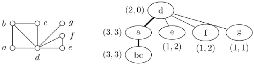
a d b c e f g d (2,0) a (3,3) bc (3,3) e (1,2) f (1,2) g (1,1)
Figure 1 A graphGand a width-3 treecut decomposition of G, including the torso-size (left value) and adhesion (right value) of each node.
the induced subgraph G[Yt]. Thedepth of a node t in T is the distance of tfrom the root
r. The vertices of ∂t =∂G(Yt) are called the border at node t. A node t 6=r in a rooted treecut decomposition isthinifadh(t)≤2 andbold otherwise. For a nodet, we letBtand
At denote the set of children oftwhich are thin and bold, respectively.
While it is not known how to compute optimal treecut decompositions efficiently, there exists a fixed-parameter 2-approximation algorithm which fully suffices for our purposes. I Theorem 3 ([24]). There exists an algorithm that takes as input an n-vertex graph G
and integerk, runs in time2O(k2logk)
n2, and either outputs a treecut decomposition ofGof width at most2kor correctly reports that tcw(G)> k.
A treecut decomposition (T,X) is nice if it satisfies the following condition for every thin node t ∈ V(T): N(Yt)∩Sbis a sibling oftYb = ∅. The intuition behind nice treecut decompositions is that we restrict the neighborhood of thin nodes in a way which facilitates dynamic programming.
ILemma 4([20]). There exists a cubic-time algorithm which transforms any rooted treecut decomposition (T,X) of G into a nice treecut decomposition of the same graph, without increasing its width or number of nodes.
The following property of nice treecut decompositions will be crucial for our algorithm. I Lemma 5 ([20]). Let t be a node in a nice treecut decomposition of width k. Then
|At| ≤2k+ 1.
We refer to previous work [20] for a comparison of treecut width to other parameters.
3
Hardness Results
In this section we show that BDD is W[1]-hard parameterized by a vertex deletion set to trees of height at most three, i.e., a subset D of the vertices of the graph such that every component in the graph, after removing D, is a tree of height at most three. On the way towards this result, we provide hardness results for several interesting versions of the multidimensional subset sum problem (parameterized by the number of dimensions) which we believe are interesting in their own right. In particular, we note that the hardness results also hold for the well-known and more general multidimensional knapsack problem [18].
Our first auxiliary result shows hardness for the following problem. Multidimensional Subset Sum (MSS)
Input: An integerk, a setS ={s1, . . . , sn}of item-vectors withsi∈Nk
for everyiwith 1≤i≤nand a target vectort∈Nk.
Parameter: k
Question: Is there a subsetS0⊆S such thatP
ILemma 6. MSSisW[1]-hard even if all integers in the input are given in unary. Proof sketch. The proof is by a parameterized reduction from the well-known W[1]-hard Multicolored Clique (MCC) problem [13]: given a k-partite graphG with partition
V1, . . . , Vk, decide whetherGcontains a clique of sizek. For an instanceI= (G, k) of MCC we construct an equivalent instance I0 = (2 k
2
+k, S, t) of MSS in polynomial time, as follows. For everyv ∈V(G) we construct one item-vectorsv in S and for every e∈E(G) one item-vector se. Furthermore, we impose the following requirements on every solution
S0 ⊆ S of I0: (1) exactly one vector s
v with v ∈ Vi is contained in S0 for every i with 1≤i≤k, (2) exactly one vector se, withebeing an edge betweenVi andVj, is contained in S0 for every i and j with 1 ≤ i < j ≤ k, and (3) for every edge e with se ∈ S0 and endpoints vi ∈ Vi, vj ∈ Vj we find svi, svj ∈ S
0. To ensure (1), the target vector has k
entries with value one and every vectorsv with v ∈ Vi has value one at the i-th of those entries. Property (2) is ensured in a similar way by using k2
entries with value one in the target vector. To ensure Property (3), we assign to every vertexv of G a unique number
S(v) from a Sidon sequence S of length |V(G)| [16]. A Sidon sequence is a sequence of natural numbers such that the sum of each pair of numbers is unique; it can be shown that it is possible to construct such sequences whose maximum value is bounded by a polynomial in its length [1, 16]. The target vector then contains one additional entryI(i, j) for every i
andj with 1≤i < j≤k with value max2(S) + 1, where max2(S) is the maximum sum of any two numbers inS. Moreover, every vectorsvforv∈V(G) has valueS(v) at every entry
I(l, r) withl=iorr=iand similarly every vector sefor an edgeebetweenVi andVj has value (max2(S) + 1)−(S(u) +S(v)) at entryI(i, j). Then, becauseS is a Sidon sequence, it holds that theI(i, j)-th entry ofP
s∈S0sfor a solutionS0 is equal to theI(i, j)-th entry
oft if and only if the endpoints of the unique edge chosen betweenVi and Vj are equal to the unique verticesvi andvj chosen inVi andVj, respectively. J The proof of the above lemma also implies hardness for the following slightly adapted ver-sion of MSS, which we call theRestricted Multidimensional Subset Sum (RMSS) problem. ForRMSSan additional integerk0 is given (which will be part of the parameter) and we ask for a solution of the MSS problem of size exactly k0. Before presenting our hardness result for BDD, we need to show hardness for the following more relaxed version of RMSS, which we call theMultidimensional Relaxed Subset Sum (MRSS) problem. ForMRSSboth the input as well as the parameters are the same as in the case of RMSS however one now asks whether there is a subsetS0⊆Swith|S0| ≤k0such thatP
s∈S0s≥t.
ILemma 7. MRSSisW[1]-hard even if all integers in the input are given in unary. We are now ready to show our main hardness result for BDD using a reduction fromMRSS. ITheorem 8. BDD is W[1]-hard parameterized by the size of a vertex deletion set into trees of height at most3.
Proof Sketch. We prove the theorem by a parameterized reduction from MRSS. Namely, given an instanceI= (k, S, t, k0) ofMRSSwe construct an equivalent instanceI0= (G, d, `)
of BDD such thatG has a FVSD of size k·k0. The core idea of the reduction relies on transforming the decision of whether to select a vector into a solution S0 for I into the decision of whether to resolve a tree gadget inGin one of two possible ways.
The setDconsists of (k0+ 1) verticesd1i, . . . , dik0+1 for everyiwith 1≤i≤k. Moreover, for every s∈ S we introduce the gadget G(s) defined as follows. G(s) consists of max(s) stars with centerscs1, . . . , csmax(s) andd+ 1 leaves. For every star with center c
s
i, we denote byls
by rs, that has an edge to every center vertex csi. Finally, we add edges between the leavesls
1, . . . , lmax(s s) and the vertices inD such that for everyi and j with 1 ≤i ≤k and 1≤j ≤k0+ 1, it holds thatdji hass[i] neighbors among the leavesls
1, . . . , lsmax(s)of G(s). Clearly this is always possible and can be done in an arbitrary manner.
We set dto be the maximum degree of the part ofGconstructed so far (note that this maximum is reached by one of the vertices inD). Moreover, we now ensure that for every
i and j with 1 ≤ i ≤ k and 1 ≤ j ≤ k0+ 1, the vertex dji has degree d+t[i] in G by attaching a appropriate number of leaves todi. Finally, we set`to be Ps∈Smax(s)
+k0. This completes the construction of I0. Clearly, I0 can be constructed in polynomial time.
Moreover, |D| ≤k·k0 and each component of G−D is a tree with height at most 3. To complete the proof, it suffices to establish the equivalence betweenI andI0.
J Clearly trees of height at most three are trivially acyclic. Moreover, it is easy to verify that such trees have pathwidth [25] and treedepth [32] at most three, which implies:
ICorollary 9. BDDisW[1]-hard parameterized by any of the following parameters: the size of a feedback vertex set,
the pathwidth and treedepth of the input graph,
the size of a minimum set of vertices whose deletion results in components of path-width/treedepth at most three.
4
Solving BDD using Treecut-width
The goal of this section is to provide a fixed-parameter algorithm forBDDparameterized by treecut-width. The core of the algorithm is a dynamic programming procedure which runs on a nice treecut decomposition of the input graph. First we define the data table the algorithm is going to dynamically compute for individual nodes of the treecut decomposition. For each node t∈T, the table is going to contain two components, which we will call the universal costutand thespecific costst. Informally, the universal cost captures the minimum number of vertices which need to be deleted fromYtto satisfy the degree bound inGt. The specific cost captures how many more vertices (than the universal cost) we need to delete in order to satisfy the degree bound in Gt when we also place restrictions on howGt will interact with the rest of the graph. We formalize these notions below.
Let us fix an instance (G, d, `) of BDDand a treecut decomposition (T,X) ofGof width at mostkand rooted atr. Aconfiguration δof a graphH with a designated vertex-subset
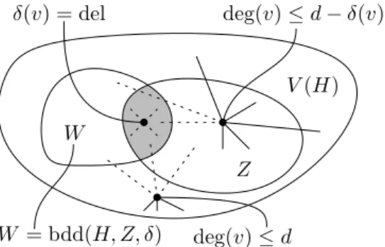
Z is a mapping Z 7→ [k]∪del. Intuitively, configurations are going to be used to place additional restrictions on the deletion sets we are interested in. We letbdd(H, Z, δ) denote the minimum size of a vertex setW ⊆V(H) such that:
v∈W∩Z if and only ifδ(v) = del, and
for eachv∈Z\W, the degree ofv inH−W is at mostd−δ(v), for eachv∈V(H)\(Z∪W), the degree of vin H−W is at mostd.
Figure 2 depicts an illustration of bdd(H, Z, δ). Informally, bdd captures the size of a minimum deletion set which intersects the designated subset precisely in the vertices specified by δ, and for the remainder of the designated subset it overshoots the degree bound by a buffer specified byδ. Ifbdd(H, Y, δ) is not defined (which may happen, e.g., ifd <|Y|), we formally setbdd(H, Y, δ) =∞. For each nodet∈V(T), we can now define:
ut=bdd(Gt,∅,∅), and
for each δ : ∂t → [k]∪del such that each v ∈ ∂t is mapped to del or to an integer
V(H) W Z δ(v) = del deg(v)≤d−δ(v) deg(v)≤d W = bdd(H, Z, δ)
Figure 2Illustration of the setbdd(H, Z, δ). The dotted edges are not considered for the de-gree of a nodev.
At ∂t
t
Bounded number of equivalence classes
Bt Bt
Figure 3The three branching sets for a node t ∈ T, first branch on ∂t (green), then on the boundaries of the bold nodesAt together with the “interior” of t (orange) and finally on the equivalence classes ofBt (gray).
We proceed with a few observations. Naturally, the value ofutcan be much larger than
k (as an example, consider a collection of disjoint stars), and this is not an issue for our algorithm. Furthermore, for everyδit holds that 0≤s0t(δ), sinceut≤bdd(Gt, ∂t, δ); notice thatutattains the value of the smallest deletion set forGt, whilebdd(Gt, ∂t, δ) attains the value of a smallest deletion set forGtwhich satisfies certain additional restrictions.
Crucially, the value ofs0t(δ) can be much larger thank, and this represents a significant obstacle for our algorithm. The role of the specific cost in the dynamic programming pro-cedure is to capture how a node may interact with the solution and how such interactions affect the size of a deletion set. The algorithm relies heavily on having only a bounded number of possible interactions in order to achieve its run-time bounds. Luckily, we will prove that any value ofs0t(δ) exceedingkmust lead to a dead end and can be disregarded. ILemma 10. LetS be a minimum-size bounded degree deletion set inG. Letδt
S be defined
over ∂t as follows: δSt(v) =del if v ∈ S, and otherwise δSt(v) = |(N(v)\Yt)\S|. Then
s0t(δt
S)≤ |N(Yt)| ≤k.
Proof. For brevity, let q = N(Yt). The fact that q ≤ k follows immediately from the bound on the adhesion oft, hence we only need to prove thats0t(δt
S) ≤q. So, assume for a contradiction that s0t(δt
S) > q. Let P be a witness for the value of ut, i.e., let P be a minimum-cardinality vertex subset of Gt such that the maximum degree inGt−P is at mostd. Observe that|P∪N(Yt)|=ut+q. Now consider the setS0= (S\Yt)∪P∪N(Yt). First of all, note that|S0|<|S|, since we obtainedS0 fromS by removing more thanu
t+q vertices (recall that, by our assumption,s0t(δt
S)> q) and then adding back at most ut+q vertices. Second, we claim that S0 is also a bounded degree deletion set in G. Indeed, consider for a contradiction thatG−S0contains a vertexvof degree higher thand. Such a
v cannot lie inYtsinceP was a solution inGtandN(Yt) separatesGtfrom the rest ofG. On the other hand,vcannot lie outside of Yt due to the fact thatS itself was a solution in
G[V(G)−Yt]. So the claim holds, andS0 contradicts the optimality ofS. J Thanks to Lemma 10, we can safely focus our attention on those configurationsδwhere
s0t(δ)≤ |N(Yt)|. Hence we definest(δ) =s0t(δ) ifs0t(δ)≤ |N(Yt)| ands0t(δ) =∞otherwise. Observe that, unlikes0t, the number of distinct possibilities of what a special costst may look like is bounded by a function ofk. The high-level strategy for the algorithm is now the following:
1. Compute (ut, st) whentis a leaf,
2. Compute (ut, st) whent is not a leaf, but the universal and specific costs are known for all of its children, and
3. Use the values (ur, sr) at the root noder∈T.
As we will see below, points1. and3. are straightforward.
IObservation 11. (ut, st)can be computed in time at most2O(k) if tis a leaf.
Proof. To compute ut it suffices to exhaustively loop through all vertex subsets L ⊆ Xt and check whether Gt−Lhas degree at most d. Thenutis equal to the minimum size of such a subset. To computest, we proceed similarly: for each configurationδsuch that each
v ∈∂t is mapped to del or to an integer i≤ |N(v)\Yt|, we exhaustively loop through all
L⊆Xt\∂t in order to determine the value ofbdd(Gt, ∂t, δ), and we then use that value
andutto determinest(δ). J
IObservation 12. (G, d, `)is a YES-instance of BDDif and only if ur≤`.
Given the above, the last remaining obstacle is handling point (2), i.e., the dynamic propagation of information from leaves to the root. This is also the by far most challenging part of the algorithm. Let us fix a nodet∈T and for all its childrenpwe assume (up, sp) to be already computed.
Our strategy is to apply a 2-step approach. Figure 3 shows an illustration of the upcoming branching sets for a nodet. Recall thatAtandBtdenote the set of all children oftwhich are bold and thin, respectively. First, we exhaustively loop over all options of how a deletion set candidate intersects withXtand the borders of nodes inAt, resulting in a set of “templates” which provide us with additional information about a potential solution. Here the bound on|At|provided in Lemma 5 will be crucial. Second, we use branching and network flows to find an optimal way of extending such a template to a solution which deals with Bt. In this step, we overcome the fact that there may be an unbounded number of childrenpinBt by “aggregating” them into types based on their sp component. Lemma 10 along with our definition of specific costs then guarantees that the number of aggregated types will depend only on k. Informally, if two nodes p1, p2 in Bt have the same specific cost, then their behavior (“contribution”) to any solution is fully interchangeable. In particular, even ifp1,
p2have different universal costs, both of these costs will need to be “paid” by every solution regardless of how the solution handles the borders of these nodes. When formalizing the above sketched algorithm we obtain.
ILemma 13. Point 2. can be solved in time2O(k2)· |B
t|2, where|Bt|is upper-bounded by
the number of children oft.
I Theorem 14. BDD can be solved in time n3+ 2O(k2·logk)
·n2, where k and n are the treecut-width and number of vertices of the input graph, respectively.
Proof. We begin by applying Theorem 3 followed by Lemma 4 to obtain a nice treecut decomposition (T,X) of width at most 2k. We then use a dynamic programming algorithm to compute the values ut and st at every node t ∈ T. For leaves, this is carried out by Observation 11, while for non-leaves we invoke Lemma 13. Finally, once we computeurfor the rootr, we can determine the answer to aBDD instance using Observation 12. J Finally, using standard techniques it is not difficult to show that BDD parameterized by treecut width does not admit a polynomial kernel.
I Theorem 15. BDD parameterized by treecut width has no polynomial kernel unless
5
Core Fracture Number
In this section we introduce the new structural parameter core fracture number and pro-vide a fixed-parameter algorithm for BDD parameterized by this parameter. An important prerequisite for the introduction of this parameter is the following simple preprocessing pro-cedure that can be applied to any BDD instance. Given an instanceI = (G, d, `) of BDD, thecore of I, denoted by c(I) = (c(G), d, `), is the BDD instance obtained from I after removing all edges whose both endpoints have degree at mostdfrom G.
IObservation 16. Let I = (G, d, `) be a BDD instance. Then I and c(I) are equivalent instances of BDD in the sense that any solution forI is also a solution for c(I) and vice versa. Moreover,c(I)can be computed in linear time w.r.t. the number of edges of G. In the following we will assume that we have already applied the above preprocessing proce-dure to any BDD instance and hence the graph of the instance does not contain any edges between vertices whose degree is already below the given degree bound. Thecore fracture number of a BDD instanceI= (G, d, `), denoted bycfn(I), is the minimum integerksuch that there is a deletion set D ⊆ V(G) with |D| ≤ k and the number of vertices in any component C of G\D of degree larger than d in G is at most k. In other words, each connected component ofG−D may contain only at mostk vertices of degree greater than
d. We start by showing that this parameter is orthogonal to treecut width.
ITheorem 17. There is a class of BDD instances with bounded treecut width and unbounded core fracture number. Similarly, there is a class of BDD instances with bounded core fracture number and unbounded treecut width. Moreover, both classes only contain BDD instancesI
withc(I) =I.
We are now ready to present our fixed-parameter algorithm for BDD parameterized by the core fracture number. The algorithm consists of two steps: (1) it computes a deletion setD
of size at mostk, witnessing thatcfn(I)≤kand (2) it solvesI with the help of the deletion setD. Namely, our algorithm will consists of fixed-parameter algorithms for the following two parameterized problems. Given an instanceI= (G, d, `) of BDD and an integerk(which also serves as the parameter of the problem), theCore Fracture Number Detection (CFND)problem, asks whether cfn(I)≤k and if so outputs a set D ⊆V(G) witnessing this. On the other hand theCore Fracture Number Evaluation (CFNE) problem asks whetherI has a solution for a given BDD instance I= (G, d, `) and a setD⊆V(G) witnessing thatcfn(I)≤ |D|and is parameterized by|D|.
ITheorem 18.CFND can be solved in timeO((2k+1)k|E(G)|)and is hence fixed-parameter
tractable. Moreover, CFND can be approximated in polynomial time within a factor of2k+1. LetI = (G, d, `, D) be an instance of CFNE and assume w.l.o.g. that c(G) =G. We start by showing that we do not need to consider solutionsV0 ⊆V(G) for I that contain more than 2k−1 vertices from any component C ofG−D.
ILemma 19. IfI has a solution, then it has a solutionV0 such that |V0∩V(C)|<2kfor every componentC ofG−D.
Proof. LetV0 be a solution forI andC be a component ofG−D with|V0∩V(C)| ≥2k;
if no such component exists, then we are done. LetM be the set of all vertices inC, whose degree is larger thandinG. Then (V0\V(C))∪M∪Dis also a solution forIand moreover
|(V0\V(C))∪M ∪D| ≤ |V0| −2k+k+k≤ |V0|. By iterating the same process for every
componentC with|V0∩V(C)| ≥2k, one obtains the desired solution forI.
LetC be a component of G−D and let M ⊆V(C) be the set of all vertices with degree larger than d in G. Then the signature of C, denoted by S(C), contains all pairs (D0,Γ) such thatD0⊆D, and Γ is the set of all pairs (o, γ) such that:
o is an integer with 0≤o <2k, and
γ : D\D0 → {0, . . . ,2k−1} is a mapping such that there is a set V0 ⊆ V(C) with
|V0|=osatisfying the following conditions:
(S1) every vertex inM \V0 has degree at mostdin G−(V0∪D0) and (S2) for every vertexvin D\D0,V0 contains exactlyγ(v) neighbors of v.
Informally, for every subset D0 of vertices that we decide to delete from D, the signature tells us how many vertices inC we need to delete and how their deletion affects the degrees of the remaining vertices inD−D0. Because we only need to consider solutions containing less than 2k vertices fromC (Lemma 19), the number of ways in which different solutions effect the degrees of vertices inD is bounded, which allows us to compute the signatures. ILemma 20. The signatureS(C)can be computed in timeO(|V(C)|+|E(C)|+ 2k(2k)22k) for any componentC of G−D.
LetD0 ⊆D andC andC0 be two distinct components ofG−D. We say thatCandC0are equivalent w.r.t. D0 if (D0,Γ)∈ S(C)∩ S(C0) for some Γ. LetP(D0) be the partition of all components ofG−Dinto equivalence classes and for an equivalence classC ∈ P(D0) let Γ(C)
denote the set Γ such that (D0,Γ)∈ S(C) for everyC∈ C. Note that|P(D0)| ≤2k(2k)k. ILemma 21. An instanceI = (G, d, `, D)has a solution if and only if there is a subsetD0
of D and a mapping αthat assigns to every C ∈ P(D0) and every (o, γ) ∈Γ(C) a natural number satisfying the following conditions:
(C1) (P
C∈P(D0)∧(o,γ)∈Γ(C)o·α(C,(o, γ))) +|D0| ≤`, i.e., the budget` is not exceeded,
(C2) P
(o,γ)∈Γ(C)α(C,(o, γ)) =|C|for everyC ∈ P(D
0), i.e., all components are considered,
(C3) P
C∈P(D0)∧(o,γ)∈Γ(C)γ(v)·α(C,(o, γ)≥ |NG−D0(v)| −d for everyv ∈D\D0, i.e., the
degree conditions for the vertices inD\D0 are satisfied.
Proof. Towards showing the forward direction letV0be a solution forI. We start by setting
D0=D∩V0. Consider a componentCofG−Dand let Γ be the set such that (D0,Γ)∈ S(C).
Because of Lemma 19, we can assume that |V0 ∩V(C)| < 2k. Hence Γ contains a pair
(|V0∩V(C)|, γ), which we denote byA(C), such that for everyv ∈D\D0, it holds that v
has exactlyγ(v) neighbors inV0∩V(C). For every C ∈ P(D0) and (o, γ)∈Γ(C), we now setα(C,(o, γ)) to be the number of componentsCinCwithA(C) = (o, γ) and claim thatα
satisfies the conditions (C1)–(C3). Because (P
C∈P(D0)∧(o,γ)∈Γ(C)o·α(C,(o, γ)))+|D0|=|V0|
and|V0| ≤`, we obtain thatαsatisfies (C1). Condition (C2) follows immediately from the
definition of α. Finally, Condition (C3) follows because for everyv ∈D\D0 it holds that
P
C∈P(D0)∧(o,γ)∈Γ(C)γ(v)·α(C,(o, γ)) is equal to the number of neighbors ofvinV0\Dand
the fact thatvcan have at mostdneighbors inG−V0.
Towards showing the reverse direction let D0 ⊆Dandαbe a mapping satisfying (C1)– (C3). For a component C ∈ C and (o, γ) ∈ Γ, where C ∈ P(D0) and (D0,Γ) ∈ S(C), we denote by V(C,(o, γ)) a subset of V(C) of size o satisfying the conditions (S1) and (S2) in the definition of a signature. Then a solution V0 for I is obtained as follows. For any
C ∈ P(D0) we take the union of V(C,(o, γ)) for exactly α(C,(o, γ)) components C ∈ C.
Condition (C2) ensures that there are enough components inC and moreover that this way we use every component exactly once. Finally, we addD0toV0. Because of Condition (C1), we have that|V0| ≤`. Moreover, because of Condition (C3), we obtain that every vertex in
D\D0 has degree at mostdin G−V0. The same holds for every vertex in any component
With the help of the above lemma, we can express the existence of a solution in terms of the solution of an integer linear program with a bounded number of variables, which in turn can be solved in fpt-time w.r.t. the number of variables [28].
ITheorem 22. CFNE is fixed-parameter tractable.
Proof sketch. Let I = (G, d, `, D) be the given instance of CFNE. The algorithm first computes the signature S(C) for every component C of G−D according to Lemma 20. It then uses the characterization given in Lemma 21 to decide whether I has a solution. Namely, for every D0 ⊆D the algorithm constructs an ILP instance I0 whose optimum is
at most`− |D0| if and only if the BDD instanceI has a solution V0 with V0 ∩D = D0.
In accordance with Lemma 21 the ILP instanceI0 has one variable, denote byx
C,(o,γ), for everyC ∈ P(D0) and (o, γ)∈Γ(C) and consists of the following constraints:
minimize X C∈P(D0),(o,γ)∈Γ(C) o·xC,(o,γ) subject to X (o,γ)∈Γ(C) xC,(o,γ)=|C| ∀C ∈ P(D0) X C∈P(D0)∧(o,γ)∈Γ(C) γ(v)·xC,(o,γ)≥ |NG−D0(v)| −d∀v∈D\D0
Observe that there is a one-to-one correspondence between assignmentsβ for the variables in I0 and the assignment αdefined in Lemma 21. Moreover, the constraints of I0 ensure
Condition (C2) and (C3) and Condition (C1) can be satisfied if and only if the optimum value ofI0 is at most`− |D0|. This completes the description of the algorithm.
J As our final result, we show a kernel lower bound for CFNE.
ITheorem 23. CFNE has no polynomial kernel unless coNP⊆NP/poly.
Proof sketch. We give a polynomial parameter transformation [2, Proposition 1] from the well-knownSet Coverproblem parameterized by the size of the universe. It is known that Set Cover does not admit a polynomial kernel unless coNP⊆NP/poly [10]. Given an instanceI = (U,F, k) of Set Cover, we construct an instance I0 = (G, d, `, D) of CFNE
as follows. Ghas one vertexvu for everyu∈U as well as one vertexwF for everyF ∈ F. Moreover,Ghas an edge between a vertexvuand a vertex wF if and only ifu∈F. We set
D={vu |u∈U}. Let ∆ be the maximum degree of any vertex inG. Then we attach to every vertex inDnew leaf vertices such that the degree of every vertex inD becomes ∆ + 1. This completes the construction ofG. Finally, we set d= ∆ and `=k. BecauseG−D is an independent set, this shows thatcfn(G)≤k. To complete the proof, it remains to show thatI has a solution if and only if so doesI0. J
6
Concluding Notes
Our results close a wide gap in the understanding of the complexity landscape of BDD parameterized by structural parameters. In particular, they not only resolve the main open question from previous work in the area [5], but push the lower bounds significantly further, specifically to deletion distance to trees of bounded depth. Moreover, we identified structural parameterizations which are better suited for the problem at hand and used these to obtain two novel fixed-parameter algorithms for BDD.
References
1 Martin Aigner and Günter M. Ziegler. Proofs from the Book (3. ed.). Springer, 2004. 2 Christer Bäckström, Peter Jonsson, Sebastian Ordyniak, and Stefan Szeider. A complete
parameterized complexity analysis of bounded planning. JCSS, 81(7):1311–1332, 2015. 3 Balabhaskar Balasundaram, Sergiy Butenko, and Illya V. Hicks. Clique relaxations in
social network analysis: The maximumk-plex problem. Operations Research, 59(1):133– 142, 2011.
4 Balabhaskar Balasundaram, Shyam Sundar Chandramouli, and Svyatoslav Trukhanov. Ap-proximation algorithms for finding and partitioning unit-disk graphs into co-k-plexes. Op-timization Letters, 4(3):311–320, 2010.
5 Nadja Betzler, Robert Bredereck, Rolf Niedermeier, and Johannes Uhlmann. On bounded-degree vertex deletion parameterized by treewidth. Discrete Applied Mathematics, 160(1-2):53–60, 2012.
6 Hans L. Bodlaender and Babette van Antwerpen-de Fluiter. Reduction algorithms for graphs of small treewidth. Inf. Comput., 167(2):86–119, 2001.
7 Zhi-Zhong Chen, Michael R. Fellows, Bin Fu, Haitao Jiang, Yang Liu, Lusheng Wang, and Binhai Zhu. A linear kernel for co-path/cycle packing. InProc. AAIM 2010, volume 6124 ofLNCS, pages 90–102. Springer, 2010.
8 Bruno Courcelle. The monadic second-order logic of graphs. i. recognizable sets of finite graphs. Inf. Comput., 85(1):12–75, 1990.
9 Marek Cygan, Fedor V. Fomin, Lukasz Kowalik, Daniel Lokshtanov, Dániel Marx, Marcin Pilipczuk, Michal Pilipczuk, and Saket Saurabh.Parameterized Algorithms. Springer, 2015. 10 Marek Cygan, Fedor V. Fomin, Lukasz Kowalik, Daniel Lokshtanov, Dániel Marx, Marcin Pilipczuk, Michal Pilipczuk, and Saket Saurabh.Parameterized Algorithms. Springer, 2015.
doi:10.1007/978-3-319-21275-3.
11 Anders Dessmark, Klaus Jansen, and Andrzej Lingas. The maximumk-dependent andf -dependent set problem. InProc. ISAAC 1993, volume 762 ofLNCS, pages 88–98. Springer, 1993.
12 Reinhard Diestel. Graph Theory, volume 173 ofGraduate Texts in Mathematics. Springer Verlag, New York, 2nd edition, 2000.
13 Rodney G. Downey and Michael R. Fellows. Fundamentals of Parameterized Complexity. Texts in Computer Science. Springer, 2013.
14 Eduard Eiben, Robert Ganian, and Stefan Szeider. Meta-kernelization using well-structured modulators. In Thore Husfeldt and Iyad A. Kanj, editors,Proc. IPEC 2015, volume 43 of LIPIcs, pages 114–126. Leibniz-Zentrum für Informatik, 2015.
15 Eduard Eiben, Robert Ganian, and Stefan Szeider. Solving problems on graphs of high rank-width. InProc. WADS 2015, volume 9214 ofLNCS, pages 314–326. Springer, 2015. 16 Paul Erdős and Paul Turán. On a problem of Sidon in additive number theory, and on
some related problems. Journal of the London Mathematical Society, 1(4):212–215, 1941. 17 Michael R. Fellows, Jiong Guo, Hannes Moser, and Rolf Niedermeier. A generalization of
Nemhauser and Trotter’s local optimization theorem. J. Comput. Syst. Sci., 77(6):1141– 1158, 2011.
18 Arnaud Fréville. The multidimensional 0-1 knapsack problem: An overview. European Journal of Operational Research, 155(1):1–21, 2004.
19 Jakub Gajarský, Petr Hlinený, Jan Obdrzálek, Sebastian Ordyniak, Felix Reidl, Peter Ross-manith, Fernando Sánchez Villaamil, and Somnath Sikdar. Kernelization using structural parameters on sparse graph classes. J. Comput. Syst. Sci., 84:219–242, 2017.
20 Robert Ganian, Eun Jung Kim, and Stefan Szeider. Algorithmic applications of tree-cut width. In Giuseppe F. Italiano, Giovanni Pighizzini, and Donald Sannella, editors, Proc. MFCS 2015, volume 9235 ofLNCS, pages 348–360. Springer, 2015.
21 Robert Ganian, Friedrich Slivovsky, and Stefan Szeider. Meta-kernelization with structural parameters. J. Comput. Syst. Sci., 82(2):333–346, 2016.
22 Serge Gaspers, Neeldhara Misra, Sebastian Ordyniak, Stefan Szeider, and Stanislav Zivny. Backdoors into heterogeneous classes of SAT and CSP. J. Comput. Syst. Sci., 85:38–56, 2017.
23 Russell Impagliazzo, Ramamohan Paturi, and Francis Zane. Which problems have strongly exponential complexity? J. Comput. Syst. Sci., 63(4):512–530, 2001.
24 Eunjung Kim, Sang-il Oum, Christophe Paul, Ignasi Sau, and Dimitrios M. Thilikos. An FPT 2-approximation for tree-cut decomposition. In Laura Sanità and Martin Skutella, editors,Proc. WAOA 2015, volume 9499 ofLNCS, pages 35–46. Springer, 2015.
25 Ton Kloks. Treewidth: Computations and Approximations, volume 842 ofLNCS. Springer Verlag, Berlin, 1994.
26 Christian Komusiewicz, Falk Hüffner, Hannes Moser, and Rolf Niedermeier. Isolation con-cepts for efficiently enumerating dense subgraphs. Theor. Comput. Sci., 410(38-40):3640– 3654, 2009.
27 Martin Kronegger, Sebastian Ordyniak, and Andreas Pfandler. Variable-deletion backdoors to planning. InProc. AAAI 2015, pages 2300–2307. AAAI Press, 2014.
28 H. W. Lenstra. Integer programming with a fixed number of variables. MATH. OPER. RES, 8(4):538–548, 1983.
29 Dániel Marx and Paul Wollan. Immersions in highly edge connected graphs. SIAM J. Discrete Math., 28(1):503–520, 2014.
30 Benjamin McClosky and Illya V. Hicks. Combinatorial algorithms for the maximumk-plex problem. J. Comb. Optim., 23(1):29–49, 2012.
31 Hannes Moser, Rolf Niedermeier, and Manuel Sorge. Exact combinatorial algorithms and experiments for finding maximumk-plexes. J. Comb. Optim., 24(3):347–373, 2012. 32 Jaroslav Nešetřil and Patrice Ossona de Mendez. Sparsity - Graphs, Structures, and
Algo-rithms, volume 28 ofAlgorithms and combinatorics. Springer, 2012.
33 Rolf Niedermeier. Invitation to Fixed-Parameter Algorithms, volume 31 ofOxford Lecture Series in Mathematics and its Applications. Oxford University Press, Oxford, 2006. 34 Naomi Nishimura, Prabhakar Ragde, and Dimitrios M. Thilikos. Fast fixed-parameter
tractable algorithms for nontrivial generalizations of vertex cover. Discrete Applied Math-ematics, 152(1-3):229–245, 2005.
35 Stephen B Seidman and Brian L Foster. A graph-theoretic generalization of the clique concept. Journal of Mathematical sociology, 6(1):139–154, 1978.
36 Paul Wollan. The structure of graphs not admitting a fixed immersion. J. Comb. Theory, Ser. B, 110:47–66, 2015.