Expected Case for Projecting Points
Sergio Cabello and Matt DeVos
Institute for Mathematics, Physics and Mechanics, Ljubljana, Slovenia E-mail: [email protected]
Bojan Mohar
Faculty of Mathematics and Physics, Ljubljana, Slovenia E-mail: [email protected]
Keywords:randomized algorithm, unit distance, closest pair
Received:June 14, 2005
Consider a set ofnpoints in the plane with the property that any pair of points is at least at distance one. We study the expected concentration of the point set after projecting it onto a random graduated line. There is a lower bound ofΩ(√nlogn)given by Matoušek in [4], and we provide an upper bound ofO(n2/3). Povzetek: Analizirana je gostota toˇck v ravnini z razdaljo najmanj ena.
1 Introduction
LetP be a set ofnpoints in the plane. For a lineL⊂R2, we can project the points P orthogonally ontoL, which we denote by πL(P). Imagine that the line Lis a
grad-uated line, that is, a line decomposed into line segments (cells) of length one. For a cell c ⊂ L, let P op(P, c)
be the population of the cellcafter the projection, that is P op(P, c) =|{p∈P|πL(p)∈c}|. For a graduated line
L, we say that its concentrationConc(P, L)is the number of points that its most populated cell gets; that is,
Conc(P, L) = max
ca cell ofL
{P op(P, c)}.
In a recent paper, Díaz et al. [3] consider the algorithmic problem of computing a graduated line that minimizes the concentration, that is, they are interested inConc(P) = minLConc(P, L). However, an asymptotically equivalent
problem was considered by Kuˇcera et al. [4] when studying a map labelling problem.
Here we are interested in the expected concentration that a point set has when projecting onto a random graduated line. LetL(α)be a graduated line through the origin with angleαwith respect to thex-axis, and such that the origin is the boundary of a cell. We are interested in the expected concentrationEConc(P)over all linesL(α)
EConc(P) =Eα[Conc(P, L(α))],
whereαis chosen uniformly at random. Let us observe that, for an asymptotic bound onEConc(P), it is equiva-lent to consider that the linesL(α)pass through some other point ofR2instead of the origin.
If the point setPis arbitrarily dense, then it may be that Conc(P, L) ≥ n/2for any lineL, and soEConc(P) = Ω(n). However, the problem becomes non-trivial if we put restrictions to the density of the point set.
Definition 1. A point setP ⊂R2is1-separatedif its clos-est pair is at least at distance 1.
Our objective1,2 is to bound the value EConc(P) for
any 1-separated point set. Kuˇcera et al. [4] have shown thatConc(P) =O(√nlogn)for any1-separated point set P. More interestingly, they use Besicovitch’s sets [1] for constructing 1-separated point setsP havingConc(P) = Ω(√nlogn), which impliesEConc(P) = Ω(√nlogn).
We will show that for any 1-separated point setP we haveEConc(P) =O(n2/3). Therefore, it remains open to find tight bounds forEConc(P).
The rationale behind considering projections onto ran-dom lines is the efficiency of ranran-domized algorithms whose running time depends on the expected concentration. As an example, consider a set of disjoint unit disks and any sweep-line algorithm [2, Chapter 2] whose running time depends on the maximum number of disks that are inter-sected by the sweep line. Choosing the direction in which the line sweeps affects the running time, but computing the best direction, or an approximation, is expensive: Kuˇcera et al. [4] claim that it can be done in polynomial time, and Díaz et al. [3] give a constant-factor approximation algo-rithm with O(ntlognt) running time, where t is the di-ameter ofP. By choosing a random projection we avoid having to compute a good direction for projecting, and we get a randomized algorithm. The results in this paper be-come helpful for analyzing the expected running time of such randomized algorithms.
The rest of the paper is organized as follows. In Sec-tion 2 we introduce some relevant random variables and give some basic facts. In Sections 3 and 4 we bound
1Supported by the European Community Sixth Framework Pro-gramme under a Marie Curie Intra-European Fellowship.
EConc(P) using the first and second moments, respec-tively.
2 Preliminaries
LetP = {p1, . . . , pn}be a 1-separated point set, and let
di,j = d(pi, pj). We use the notation[n] = {1, . . . , n}.
Without loss of generality, we can restrict ourselves to graduated lines passing through the origin. LetL(α)be the line passing through the origin that has angleαwith thex -axis, and letp∗(α)be the orthogonal projection of a point
pontoL(α). Consider the following random variables for the angleα
Xi,j(α) =
(
1 ifd¡p∗
i(α), p∗j(α)
¢ ≤1,
0 otherwise;
Xi(α) = n
X
j=1
Xi,j(α);
Xmax(α) = max{X1(α), . . . , Xn(α)};
X(α) =
n
X
i=1
Xi(α) = n
X
i=1
n
X
j=1
Xi,j(α),
where αis chosen uniformly at random from the values
[0, π). In words:Xi,jis the indicator variable for the event
thatp∗
i(α)andp∗j(α)are at distance at most one in the
pro-jection; Xi is the number of points (including pi itself)
whose projection is at distance at most one from p∗
i(α);
Xmaxis the maximum amongX1, . . . , Xn; andX counts
twice the number of pairs of points at distance at most one in the projection. It is clear thatP[Xi,i = 1] = 1for any
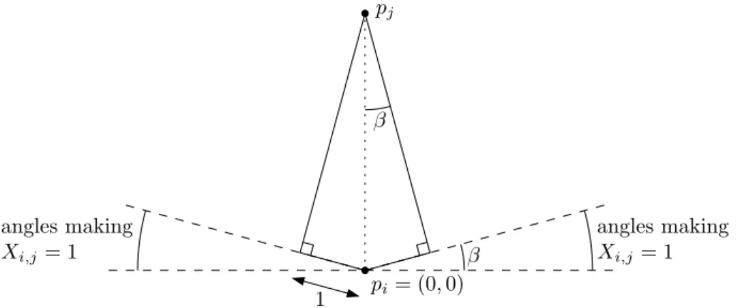
i∈[n]. Otherwise we have the following result. Lemma 1. Ifi6=j, then
P[Xi,j= 1] = 2 arcsin 1/di,j
π .
Proof. Assume without loss of generality thatpiis placed
at the origin andpjis vertically above it, on they-axis. See
Figure 1. We may also assume that the lineL(α)passes through pi. Because di,j ≥ 1, there are values α such
that Xi,j(α) 6= 1. The angles that make Xi,j(α) = 1
are indicated in the figure. In particular, ifβ is the angle indicated in the figure, and we chooseαuniformly at ran-dom, thenP[Xi,j = 1] = 2πβ. The angleβ is such that
sinβ = 1
di,j, and soβ = arcsin 1
di,j. We conclude that P[Xi,j= 1] = 2πβ = 2 arcsin 1π /di,j.
The first observation, which is already used for the ap-proximation algorithms described by Díaz et al. [3], is that, asymptotically, we do not need to care for the graduation, but only for the orientation of the line. In particular, the random variables Xi contain all the information that we
need asymptotically. Lemma 2. We have EConc(P))
2 ≤E[Xmax(α)]≤2EConc(P).
3 Using the first moment
Using that the closest pair ofPis at least one apart, we get the following result.
Lemma 3. For everyi∈[n], we have
X
j∈[n]\{i}
1 di,j =O(
√
n).
Proof. Without loss of generality, assume thati =n. Let ndbe the number of points inPwhose distance frompnis
in the interval[d, d+ 1). We have
X
j∈[n−1]
1 di,j =
∞
X
d=1
X
di,j∈[d,d+1)
1 di,j
(1)
≤
∞
X
d=1
X
di,j∈[d,d+1)
1 d
(2)
=
∞
X
d=1 nd
d. (3)
Observe that if we have two sequences(ai)i∈Nand(bi)i∈N of nonnegative numbers such thatPji=1ai ≤
Pj i=1bifor
all j ∈ N, then P∞i=1 ai
i ≤
P∞
i=1bii. That is, the sum
is maximized when the values concentrate on the smallest possible indexes. LetNd be the maximum number of
1-separated points that you can have in an annulus of inner radiusdand exterior radiusd+ 1, and letDbe the smallest value such that n < PDd=1Nd. We haven =
P
ndand
Pj
i=1ni ≤
Pj
i=1Ni for all j ∈ [D], and from (1) we
conclude
X
j∈[n−1]
1 di,j ≤
∞
X
d=1 nd
d ≤
D
X
d=1 Nd
d . (4)
We need to estimate the valuesNd. For the lower bound,
placing points at distance one in the circle of radiusd, we getNd = Ω(d). For the upper bound, we can use a
pack-ing argument to show that any 1-separated point set inside the annulus has O(d)points. Indeed, if we place a disk of radius1/2centered in each point of a 1-separated point set inside the annulus, they must have disjoint interiors and cover an area ofΘ(Nd). Moreover, all these disks are
con-tained in an annulus of inner radiusd−1and exterior ra-diusd+ 2, which has an area ofΘ(d). We conclude that Nd= Θ(d), and thereforeD=O(
√
n). Using (4) we get
X
j∈[n−1]
1 di,j ≤
D
X
d=1 Nd
d ≤
OX(√n)
d=1 O(d)
d =O(
√
n).
pi= (0,0)
pj
1
angles making
Xi,j= 1
angles making
Xi,j= 1
β
β
Figure 1: For Lemma 4. We consider what random linesL(α)throughpithat giveXij = 1
Proof. BecauseXi =
Pn
j=1Xi,j and the linearity of the
expectation, we have
E[Xi] = n
X
j=1
E[Xi,j] = n
X
j=1
P[Xi,j= 1]
= 1 + X
j∈[n]\{i}
P[Xi,j= 1]
= 1 + X
j∈[n]\{i}
2 arcsin(1/di,j)
π .
Observe that the function arcsin(x) is convex for x ∈ [0,1], and therefore we have arcsin(x) ≤ (π/2)xfor all x∈[0,1]. We then have
E[Xi] = 1 +
X
j∈[n]\{i}
2 arcsin(1/di,j)
π
≤1 + X
j∈[n]\{i}
1 di,j
,
and using Lemma 3 we conclude that E[Xi] = O(
√
n).
Using the first moment method, we can show that for any 1-separated point set P it holds that EConc(P) = O(n3/4). For this, consider a 1-separated point setP and its associated random variable X. We haveX = PXi,
and because of Lemma 4 we concludeE[X] =O(n√n). We claim that, for any value t > 0, if we have Xmax(α) ≥ t, thenX(α) ≥ t2/4. Intuitively, if some
Xi =t, then there areΘ(t2)pairs of points at distance at
most one from each other, and so contributing toX. The formal proof of the claim is as follows. Letibe an index such that Xi(α) ≥ t. Then, either to the right or to the
left ofp∗
i(α), the projection ofpiontoL(α), there are at
leastt/2pointsp∗
j(α)at distance at most one fromp∗i(α).
Assume that those points are to the left and letP˜ ⊂ P be the set of those points. We have |P˜| ≥ t/2. For any pj, pj0 ∈P˜ we haveXj,j0(α) = 1, and therefore we have
Xj(α)≥t/2for allpj∈P˜. We conclude that
X(α)≥ X
pj∈P˜
Xj(α)≥
X
pj∈P˜
t/2≥t/2· |P˜| ≥t2/4,
and the claim is proved.
We have shown that for any valuet >0we have
[Xmax≥t]⊆[X≥t2/4],
and using Markov’s inequality we conclude
P[Xmax≥t]≤P[X≥t2/4]≤4E[X]
t2 ≤
O(n√n) t2 .
Letr = bn3/4c. Since X
max only takes natural
num-bers, we have
E[Xmax] = n
X
t=1
P[Xmax≥t]
=
r
X
t=1
P[Xmax≥t] + n
X
t=r+1
P[Xmax≥t]
≤
r
X
t=1
1 +
n
X
t=r+1
O(n√n) t2
≤r+O(n√n) Z n
r
1 t2dt
≤n3/4+O(n√n)
µ 1 r−
1 n
=O(n3/4).
Using Lemma 2 it follows that EConc(P) = O(n3/4). However, observe that this bound will be improved in next section.
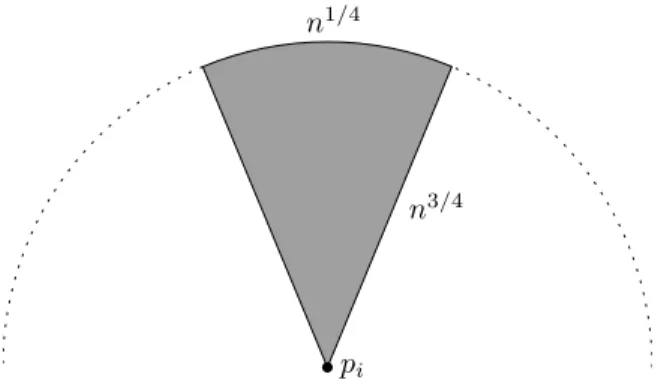
We would like to point out that the random variables Xi do not have a strong concentration around their
n3/4 n1/4
pi
Figure 2: Example showing thatXiis not concentrated around its expectation.
radius n3/4, and we consider a circular sector with arc-length n1/4. This region is grey in the picture. Imag-ine that we place a densest 1-separated point set P in-side the grey region. Asymptotically, since the region has areaΘ(n), such a point setP hasΘ(n)points. Consider the linesL(α+π/2) passing through pi. Ifαis chosen
uniformly at random, the lineL(α)intersects the grey re-gion with probability n1/4/(2πn3/4) = Θ(1/√n), and in that caseXi(α+π/2) = Θ(n3/4). We conclude that
E[Xi] = Θ(n1/4), butP[Xi= Ω(n4/3)] = Θ(1/
√
n), and soXidoes not concentrate around its expectation.
4 Second moments
Lemma 5. For everyi∈[n]we haveE[X2
i] =O(n).
Proof. Assume without loss of generality thatdi,j ≥di,k
wheneverj > k; that is, the points are indexed according to their distance frompi. Like above, we assume that the
lineL(α)passes throughpi. We have
E[X2
i] =E
X
j,k∈[n]
Xi,jXi,k
≤E
2X
j
X
k≤j
Xi,jXi,k
= 2X
j
E
Xi,j X
k≤j
Xi,k
We claim thatE
h
Xi,j
P
k≤jXi,k
i
= O(1), and so the result follows.
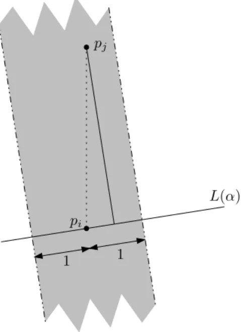
To prove the claim, observe that if Xi,j(α) = 1, then
all the pointspk that haveXi,k(α) = 1need to be in the
strip (or slab) of width two having L(α+π/2) as axis; see Figure 3, where this strip is in grey. Because of a packing argument, in this strip there areO(di,j)pointspk
that satisfy di,j ≥ di,k. Therefore, by the way we
in-dexed the points, we conclude that, ifXi,j(α) = 1, then
³P
k≤jXi,k
´
(α) =O(di,j). In any case, we always have
³
Xi,j
P
k≤jXi,k
´
(α) =O(di,j). Therefore
E[Xi,j
X
k≤j
Xi,k ] = n
X
t=1 t·P
Xi,j X
k≤j
Xi,k =t
≤
n
X
t=1
O(di,j)·P
Xi,j X
k≤j
Xi,k=t
=O(di,j) n
X
t=1 P
Xi,j X
k≤j
Xi,k=t
≤O(di,j)·P[Xi,j = 1]
=O(di,j)2 arcsin 1/di,j
π =O(1). This finishes the proof of the claim and of the lemma. Theorem 1. For any 1-separated point set P we have EConc(P) =O(n2/3).
Proof. LetP be a 1-separated point set and consider the random variableT(α) = ¡PiX2
i
¢
(α). By Lemma 5 we haveE[T] = PiE[X2
i] = O(n2). The rest of the proof
resembles the argument in the previous section.
We claim that, for any value t > 0, if we have Xmax(α)≥t, thenT(α)≥t3/8. The proof is as follows.
Letibe an index such thatXi(α)≥t. Then, either to the
right or to the left ofp∗
i(α), the projection ofpiontoL(α),
there are at leastt/2pointsp∗
j(α)at distance at most one
fromp∗
i(α). Assume that those points are to the left and let
˜
P ⊆P be the set of those points. We have|P˜| ≥t/2. For anypj, pj0 ∈ P˜ we haveXj,j0(α) = 1. Therefore for all
pj ∈ P˜ we haveXj(α) ≥ t/2, andXj2(α) ≥ t2/4. We
conclude that
T(α)≥ X
pj∈P˜ X2
j(α)
≥ X
pj∈P˜
t2/4≥t2/4· |P˜|
≥t3/8,
pi
pj
L(α)
1 1
Figure 3: For the proof of Lemma 5. For any angleαwe have
³
Xi,j
P
k≤jXi,k
´
(α) =O(di,j).
We have shown that for any valuet >0we have
[Xmax≥t]⊆[T ≥t3/8],
and using Markov’s inequality we conclude
P[Xmax≥t]≤P[T ≥t3/8]≤8E[T]
t3 ≤ O(n2)
t3 .
Letr = bn2/3c. SinceX
max only takes natural
num-bers, we have
E[Xmax] = n
X
t=1
P[Xmax≥t]
=
r
X
t=1
P[Xmax≥t] + n
X
t=r+1
P[Xmax≥t]
≤
r
X
t=1
1 +
n
X
t=r+1 O(n2)
t3
≤r+O(n2) Z n
r
1 t3dt
≤n2/3+O(n2)
µ 2 r2 −
2 n2
=O(n2/3).
Using Lemma 2 it follows that EConc(P) = O(n2/3).
Trying to use the same ideas with higher moments of Xi does not help. Consider for example the 1-separated
point set P consisting of allnpoints in a horizontal row of length n, and let p1 be the leftmost point. We have
E[X3
1] = Θ(n2), and in general E[X1p] = Θ(np−1) for all naturalsp >2. From this we can only conclude weaker results of the typeEConc(P) =O(np/(p+1)).
Conclusions
We have studied the expected concentration of project-ing 1-separated point sets onto random lines, a parameter that is relevant for sweep-line algorithms when the direc-tion for sweeping is chosen at random. We have shown that, ifP consists of npoints, the expected concentration EConc(P)isO(n2/3), while the best known lower bound isΩ(√nlogn). Therefore, it remains to close this gap.
Acknowledgements
The authors are grateful to Jiˇrí Matoušek for the key ref-erence [4]. Sergio is also grateful to Christian Knauer for early discussions.
References
[1] A. S. Besicovitch. The Kakeya problem.The American Mathematical Monthly, 70:697–706, 1963.
[2] M. de Berg, M. van Kreveld, M. Overmars, and O. Schwarzkopf. Computational Geometry: Algo-rithms and Applications. Springer-Verlag, Berlin, Ger-many, 2nd edition, 2000.
[3] J.M. Díaz and F. Hurtado and M. López and J.A. Sell-arès. Optimal point set projections onto regular grids. In T. Ibaraki et al., editor,14th Inter. Symp. on Algo-rithms and Computation, volume 2906 ofLNCS, pages 270–279. Springer Verlag, 2003.