RESETting Timed Machines
Ariel Stulman
Computer Science Department, Jerusalem College of Technology, Jerusalem, Israel
Many real-time applications enableRESETto account for all kinds of unexpected problems, or to accommodate for a users’ want of restarting. Additionally, some software testing techniques must allow for resetting timed-Implementations Under Test (t-IUT). Dedicated internal logic is probably the most common of solutions for accomplishing such tasks. There are situations, however, where such a privilege doesn’t exist; thus, it cannot be built upon. Testing pre-engineered timed-IUTs is one such case. In this paper we wish to present an algorithm for the direct generation of timed RESET sequences from the timed-IUT specification, such that it should be optimal w.r.t. to execution time.
Keywords: D.2.4 [Software Engineering]: Software/-Program Verification – Formal Methods; F.1.1[Theory of Computation]: Models of Computations – Automata; D.2.m [Software Engineering]: Miscellaneous – Real-time systems
1. Introduction and Related Work
Many algorithms were devised for specific tasks within the conformance testing envelope(status messages[10], separating family of sequences, distinguishing sequences [13], UIO sequences [1],[28], characterizing sequences[11],[19],[25], and identifying sequences [19]; a survey of the main methods can be found in[24]). The abil-ity to reset the implementation under test(IUT) to its original state, however, must also be part of the algorithmic suite when testing a system or some communication protocol. This is true, whether we are interested in testing a specific state transfer or when verifying complete con-formance to specification. Not always can we rely on the existence of some magicalRESET
but-ton for this purpose. Therefore, a special type of sequence, aRESETsequence(a.k.a.
synchro-nizing sequence)was devised. It is a sequence that uses inherent transfers within the IUT to
achieve its purpose. See Kohavi’s book[19]for basic algorithm and results.
Due to the wide use of finite state machines (FSM)as the modeling technique for theIUTs,
its inherent flaw was automatically projected into system testing. Standard FSMs do not take into account temporal constraints that may in-fluence theIUT; and as such, most methods
de-veloped for system testing were not applicable to real-time systems. With the proposal of Alur and Dill’s ‘Timed automata’[3]in 1994, an en-tirely new field of system testing for real-time (reactive)systems emerged. It soon became the prevalent model for real-time systems, and the underlying theory behind many model check-ing tools; e.g., UPPAAL [23] and KRONOS [8].
The emerging field quickly became a thriving research area with many diverse sub-topics(see [5],[6],[7],[9],[21],[22],[26]],[27],[28], and many others).
Papers dealing specifically with state identifi-cation sequences, however, were not concerned with actually producing algorithms for usage on anIUTwith timing constraints(t-IUT). Their
main objective was in demonstrating how a t-IUT
can be transformed into a regular, un-timedIUT,
given in [30]. This algorithm will be extended as to provide the ability of RESETting a timed IUT without insertion of explicit reset logic as
would be required otherwise. Thus, the con-tribution of this paper is twofold: development of timed synchronizing sequence optimal with respect to execution time, and extension of the algorithm as to provide for an internal RESET
logic where possible.
2. Preliminaries
2.1. Modeling time
The notion of time can be described asdiscrete
or dense [3]. In a discrete timing model, time
increases monotonically by some constant de-cided upon a priori(usually 1)every cycle of the system. When such is the case, there is no need for a real clock. A variable that represents the current “time” is sufficient. Using such a model limits the accuracy with which physical systems can be modeled.
A more natural model for physical processes op-erating over continuous time is the dense-time model. When we talk about “real” timing of systems, we must have a clock that keeps the time. The advancement of the clock is irrespec-tive of the cycle time of the system, and can increase monotonically without bound.
Assumption 1: We use a discrete-time model in the rest of this discussion. This will allow us to use numerical values in the examples and dis-cussions. This assumption will be lifted later, in Section 4.8. [Justification: Physical hardware of computer systems functions in discrete cy-cles, so the use of a discrete-time model is more in-tune with hardware. In addition, by choosing a very small granulation value, we can approx-imate a physical system to within any accuracy level.]
2.2. I/O Automata
There are many variants of FSMused to model
systems. The majority of the state identifica-tion techniques discussed in the literature are based on the Mealy machine[16]. This fact is based upon the ability of the Mealy machine to exchange messages(input and output)with its
environment. Adeterministictransition is stim-ulated by input from the environment, and as a consequence, the machine can return an output message back to the environment (a reactive
machine). Since ablack boxtesting model[17] – where one cannot see the internal structure of the IUT, but has access to its input and output
ports – is the basic premise of checking exper-iments, the Mealy machine [19] is a suitable candidate for representing the internal logic of anIUT.
Definition 1 (Mealy Machine). A Mealy ma-chine, M is a 6-tupleS,s0,I,O,,, where:
• Sis a finite set of states.
• s0 ∈Sis the initial state of the system.
• I is a finite set of input events (I ={1,2, . . . ,p}).
• Ois a finite set of output events (O={o1,o2, . . . ,or}).
• is the state-transfer function ( :S×I →S).
• is the output function( :S×I →O). For simplicity, we extend the state transfer func-tion, , from single input symbols to input strings as follows: for some initial state s1,
let the input sequence = 1 ·2 ·. . .· k
take the machine successively through the states
sj+1 = (sj,j), where j = 1,2, . . . ,k, such that the final state of (s1,) = sk+1. In
the same manner we extend the output func-tion,, from a single output to an output string such that: (s1,) = 1·2·. . .·k, where j = (sj,j)withj = 1,2, . . . ,k. Obviously,
sj∈S,j∈Iandj∈O.
2.3. State uncertainty
It may be the case that some state information of anIUTis missing. Thestate uncertaintyof the IUTis defined as the set of states that may
ade-quately complete the missing state information [19]. If the initial state of theIUTis unknown, we
speak of aninitial state uncertainty; a set con-taining all possible states that may constitute theIUTs initial state. For example, consider the
automata in Figure 1 representing a simplified internal logic of a sender using the alternating bit protocol (ABP) for data-link layer network
of the machine, the possible transfers between these states, and the output (o ∈ O) generated by a transfer triggered by input ( ∈ I) in the form of /o on its label. If the machine can begin in any of the four states, we say that the
initial state uncertaintyis{ABCD}.
Figure 1.Automata representation of alternating bit protocol.
When the current state of theIUTis unknown, we
speak of a current state uncertainty set. Sup-pose, for example, that =ack1. After in-putting of into the IUT in Figure 1, {ABC}
will be thecurrent state uncertainty.
2.4. Successor tree
Asuccessor treeis a tree representing the states
that can be reached by theIUTbased on all
possi-ble input combinations. The purpose of the tree
is to graphically display the nthsuccessors of the root; constituting an aid in the selection of the most suitable input sequence to meet required goals.
The root of the tree contains the initial state of theIUT. When it is not known, we associate with
the root aninitial state uncertaintyvector. Tree edges represent input to theIUT. Every node is
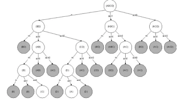
associated with acurrent state uncertainty vec-tor representing accumulated state uncertainty knowledge until that point, with being the concatenation of labels on the edges that form the path from the root to the node. For exam-ple, a partially extended successor tree for the automata in Figure 1 with an initial state uncer-tainty of{ABCD}is shown in Figure 21. Since the degree of the tree is |I|, the number of acceptable inputs in the language of the au-tomata, at levelj(0≤j ≤ ∞)we may have|I|j nodes. It is quite obvious that in order to reduce the size of the successor tree, some restrictions must be placed(avoid redundancy, etc.).
2.5. Timed I/O Automata
In this work we define a timed automaton as a Mealy machine with the addition of tempo-ral constraints on the transition function . A transition cannot fire, and hence no output or in-ternal state change can occur if the clock guard
Figure 2.Partially extended successor tree for alternating bit protocol.
1Nodes in the tree were grayed when redundancy was found. We didn’t extend those nodes as one can tell how these sub-trees
on the transition is not satisfied. Intuitively, a clock or set of clocks must be included within the system to allow for the definition of time.
Definition 2 (Clock Constraint). Let a clock constraint,, over an internal set of clocks, C, be defined as a Boolean expression of the form
copz, wherec∈C, op is a classical relational operator(=,≤,≥, >, <,=), andz∈Z≥0.
Definiton 3 (Clock Guard). Let aclock guard, , overCbe a conjunction of clock constraints overC: ( = 1∧2∧. . .∧m). Let be
the set of possible clock guards pertaining to the system, and k ⊆ be the set of all clock guards that contain at mostkclock constraints.
Definition 4 (Clock Assignment). Let a clock assignment, , over C be a conjunction of as-signments of values to some (or all) of the clocks inC, and letbe the set of all such con-junctions: ={c1 =r1∧. . .∧cm =rm|ci∈
C⊆C∧ri ∈Z≥0∧1≤m≤ |C|∧∀ci,cji=j}.
Definiton 5 (Timed I/O Automata). A timed
i/o automata, TA, is a tuple
S,s0,I,O,C,,,, where:
• Sis a finite set of states.
• s0∈Sis the initial state of the system.
• Iis a finite set of input events (I ={1,2, . . . ,p}).
• Ois a finite set of output events (O={o1,o2, . . . ,or}).
• Cis a finite set of clocks.
• is the set of clock guards pertaining to the system(see definition 3).
• is the state transfer relation ( :S×I× →S).
• is the output relation ( :S×I×→O×).
Assumption 2. For simplicity, we assume that if TA receives k ∈ I at instant t, it will also output the corresponding ob ∈ O at that ex-act instant. [Justification: In essence, output is produced on a transition generated by the in-put. Reducing transition time to be infinitely small, we may consider the input and output as occuring at the same instant.]
Assumption 3. For simplicity, we assume that |C| = 1, that : S ×I × 1 → S and that : S×I ×1 → O×2. The single clock
limitation will be lifted in Section 4.7.
2.6. Sequence generation environment
There are many possible environments within which we can develop a timed-RESETalgorithm.
The current work, however, is concerned with
theblack box modelin which we will not have
access to the internal logic of some IUT. We only have its specification model in terms of
TA, so we must deduce the required information
from it so it can be applied to an implementa-tion. Use of this environment is chosen partially because the sequence we are interested in also pertains to conformance testing, for which use of this environment is quite common.
In addition, given the following definitions:
Definition 6 (Fully specified). There exists a definition for each state, sj ∈ S, and every input, k ∈ I [and for TA for all h ∈ ];
i.e.: (sj,k) and (sj,k) [(sj,k,h) and (sj,k,h) – resp.] are defined ∀(sj,k) ∈
S×I[∀(sj,k,h)∈S×I×– resp.].
Definition 7 (Strongly connected). For every pair of states,si,sj ∈S, there exists an input se-quence[timed input sequence],ij[t-ij– resp.], which takes the automata[TA– resp.] fromsito
sj; i.e.(si,ij) =sj[(si,k,h) =sj– resp.].
Definition 8 (Reduced). For every pair of states,si,sj ∈S, there exists an input sequence, , which distinguishes them; i.e.: (si,) = (sj,) or (si,) = (sj,) [for TA: (si,,h) = (sj,,h) and the state ele-ments of (si,,h) and (sj,,h) are not equal]for some.
Definition 9 (Deterministic). Within Mealy machines determinism is inherent. To defineTA
as deterministic it must hold that ∀(sj,k,h) (sj,k,g)∈S×I×,handgare mutually exclusive; i.e.,h∧gis unsatisfiable.
Assumption 4. We assume that in the current context sequence generation and possible test-ing is performed on a fully specified, strongly
2This says that we will talk about a TA that has a single clock and that each clock guard on its transfers contains at most one
connected, reduced and deterministicIUT or t-IUT. [Justification: This is very common
as-sumptions made in literature dealing with the basic problem (see [25], [29], [5] and others). Obviously, there are works that deal with lifting any or all of these assumptions.]
3. RESET Sequence – Problem and Solution
3.1. Problem description
During the lifetime of most machines or soft-ware, the need for (self) RESETing is widely
acceptable. Within the context of protocol or system testing this feature must also be avail-able. One cannot begin execution of any test sequence without first bringing theIUTto some
identified state from which we know how to proceed. The state must be unequivocally iden-tified, regardless of the current state of theIUT.
ThisRESEToption can be realized using a
spe-cific transfer of the machine from every possible state to a predefined state; thus, achieving RE -SET. This solution will add an additional
trans-fer in our automaton from every state, compli-cating circuit or programming logic as a conse-quence. We wish to construct aRESETsequence
that will utilize existing transfers within the ma-chine while achieving an identical solution.
Definition 10 (RESET Sequence). An input sequence, RSk, is said to be a RESETsequence
(RS)of machineM, if the final state ofM after
insertion of RSk iss0(or some other state
des-ignated as aRESETstate)regardless of the initial
state prior to initiation ofRSk. LetRSk be the
set of allRSSaccepted byMas a solution to the RESETproblem; thusRSk ∈RS.
Definition 11 (Optimal Reset Sequence). We classify aRSfor machineMasoptimal,RSop, if
for allRSS,RS, accepted byM,RSopis shortest.
i.e.{|RSop| ≤ |RSk| ∀RSk ∈RS}.
3.2. Sequence generation
The RESET sequence can be easily generated
by extending the well known synchronizing se-quence(SS) (which brings the machine to some
known state) [19] concatenated with an addi-tional sequence to compensate for the transfer to theRESETstate. This method, however, doesn’t
necessarily foster the development of the opti-mal solution,RSop. We could, however, utilize
and extend the algorithm described in [19] for generating aSSusing a truncated successor tree
to reach an optimal solution as well:
Definition 12 (Synchronizing Tree). A
syn-chronizing tree(ST)is a successor tree in which
we deem a node as terminal(leaf)when one of the following occurs:
1. The loop rule: Thecurrent uncertainty as-sociated with the node was already associ-ated with a node in a preceding level. 2. The redundancy rule: Thecurrent
uncer-tainty associated with a node is also
asso-ciated with other nodes on the same level. One is chosen as a non-terminal candidate for future expansion of the tree; the others are deemed terminal.
Using a breadth first search(BFS)algorithm, we
look for a non-terminal node(leaf)that contains a singleton. The SSis constructed by
concate-nating the labels on the edges of theSTleading
from the initial uncertainty (root) to the first
node found satisfying the search criterion. Clearly thelengthof theSSis equal to the depth
of the solution node within theST. Since the first
node that can guarantee a solution was used, by the definition of BFS no other node exists at a
higher level of the tree that can also satisfy our requirements. This implies that there is no SS
with a shorter path; thus, the SS found is an
optimal synchronizing sequence.
Continuing the BFS as the method for tree
ex-pansion – until we encounter a node containing the singleton considered as theRESETstate (s0
in Definition 5)- will also solve for the optimal
RESETsequence for programs or circuits.
[19 §13.1] showed that the length of the syn-chronizing sequence, assuming it exists, is no longer than 1
2(n −1)2n. Since we can aug-ment theSS with a reset directing sequence of
no longer than(n−1)to reach theRESETstate,
we are guaranteed that the sequence is no longer than 1
2(n−1)2n+ (n−1). Thus, our algorithm is bound(in the worst case), by this value3.
3Actually, this bound isn’t tight.[19§Appendix 13.1]showed that the tight bound is1
3.3. ST Example
To demonstrate the usage of this method, we will use the alternating bit protocol of Figure 1. It was suggested that “the protocol may be ini-tialized by sending bogus messages and acks with sequence number 1. The first message with sequence number 0 is a real message”. [2]Using the tree in Figure 2, it is easy to deduce that the sender can be initialized(brought to state A) us-ing input of ’m.ack0.m.ack1’(with ’m.ack0.m’ also being a synchronizing sequence – to state D).
4. RESET Sequence for Timed Machines – Problem and Solution
The problem ofRESETting aTAis essentially the
same; mainly, to optimally bring theTAto some
pre-defined RESET state (normally s0) without
the use of a specific RESET logic. In contrast
to regular automata, we must take into account the timing constraints that restrict transitions. Some transitions may be applicable only at spe-cific times and inapplicable at others. The RS
must contain the timing of the inputs as well, so we can coordinate the input to meet the con-straints on transitions.
4.1. Context and contribution
As mentioned earlier, previous related work dealt mainly with the transformation ofTAs into
regular automata for which solutions pre-exist ([7],[18],[29]and others). In[20], for example, the transformation is done in a three step pro-cess: (1)compute the product of the automaton with a Tick automata which models the tester’s timing. The result of this combination (2) is used to generate a time-abstracting bisimula-tion quotient graph, which is similar to the well known region graph presented in[3]. Lastly, this graph is transformed into a non-deterministic Mealy machine for which all algorithms already exist. Only [30]provided an algorithm for the direct generation of synchronizing sequences forTAs. The idea was to adaptSTs for the
extrac-tion of optimal timed-synchronizing sequences by introducing the timing parameters into the tree itself.
The main drawback with the above algorithm, however, was the use of the old definition for sequence optimality; mainly, minimal sequence length. Optimality for TAs state
identifica-tion experiment sequences should be defined in terms of execution time[14]. When a time con-straint is attached to every input event, equal length sequences do not necessarily complete within the same amount of time. It is quite pos-sible that longer sequences complete faster than shorter ones. Does it really matter if we have fewer inputs if the total time for execution is elongated?
In addition, especially whenRESETting systems
is in question, the basic premise that is to be done during its’ execution. Generating a se-quence that is optimal on paper, is by no means optimal for the system users.
4.2. Optimal t-RSw.r.t. execution time
Definition 13 (Timed- RESET Sequence). A
timed- RESET sequence(t-RS), t−RSm, is a RS
that includes timing of input. t−RSm is of the
basic form 1[1]· 2[2]. . .k[k]; where, p ∈I andq ∈. Lett−RSbe the set of all timedRSs accepted by aTAas a solution to the RESETproblem; thus,t−RSm ∈t−RS.
Definition 14 (Sequence Execution time). The execution time of a sequence,, is determined by the minimum4 time that must elapse before
a sequence can be inputted in its entirety.
Definition 15 (Optimal timed-RESETsequence).
A timedRESETsequence,t−RSop, is considered
optimal w.r.t. execution time if
{t−RSop ≤t−RSm|∀t−RSm ∈t−RS}.
Consider, for example, a RESET sequence
t−RS1 = 1[c < 2] · 2[c ≥ 7]. This
se-quence must allow for clock c ∈ C to reach 7 before it can terminate (t−RS1 = 7). A
second solution sequence, t−RS2 = 1[c =
1]· 2[c < 3]·3[c ≥ 3] ·4[c = 6], must
terminate whenc ∈C reaches 6(t−rs2 = 6).
By definition 15,t−RS2 is optimal even though
|t−RS2|>|t−RS1|.
4 We used the term minimum because constraints can be composed of inequalities that allow for flexibility of input
4.3. Points to notice
The nature of applying theRESETsequence to a
timed machine would stipulate that it is insuffi-cient to bring the machine solely to its original state(s0, for example). Rather, the clocks of the
machine must also be brought to their original values as well.
Our first attempt at a possible solution is com-posed of some RESET sequence that brings the
machine to its initialized state (SRS) and has a special input (RS) that will give the clocks their initial value as well(RS). This will allow for that addition of a single edge to the machine (see Figure 3), as opposed to numerous edges proportional to the number of states.
Figure 3.Additional clock reset edge.
If possible, we would like to avoid even such a minute addition to the machine. This can be accomplishedif and only ifan edge exists from some statesktosRSsuch that it consists of some arbitrary output and the clock assignmentRS. We can search for a timed synchronizing se-quence to statesk, and then concatenate the last transfer tosRS5. If a number of such edges exist, we must find the optimal one so that the entire sequence can be declared optimal.
4.4. Generating t−RSop
In order to generate a timed RESET sequence,
we can adapt the synchronization algorithm for extraction of sequences. We are required, how-ever, to do a major overhaul if it’s to be used for optimality w.r.t. execution time. Even though the first node found during aBFSrepresents the
shortest sequence (see 3.2 and [30]), it does not necessarily represent the fastest executing sequence. Consequently, a different tree ex-pansion algorithm must be used. In addition, the rules governing efficiency vis-`a-vis the tree pruning mechanism must also change to tolerate future possible run-time developments:
Definition 16 (Timed Successor Tree). A timed successor tree is a successor tree with the addition of time constraints on its edges[30]. These time constraints are inequalities that group similarly behaving time values. The use of in-equalities allows for the avoidance of node/state explosion(see [27] and[29] pertaining this is-sue). These inequalities must be extracted from the constraints on theTA’s edges. Technically,
we must have a coupling of possible input with each possible constraint in order to allow for all possible input/time combinations. Practically, however, we can group constraints based on in-put, which further reduces the possible combi-nations needed.
For example, in theTAof Figure 4, the
inequali-ties that “cover” the different possible groupings arec ≤ 2, 2 < c < 3, c = 3, 3 < c < 4and,
c ≥ 4. All other groupings might introduce non-determinism into our model. If we group the constraints based on inputs, however, we can minimize the possible combinations with-out introducing non-determinism. Thus, we get
c < 3, c = 3, 3 < c < 4 and, c ≥ 4 for the input of 0, andc≤2and c>2 for the input of 1 – these values are used in Figure 5.
Similarly to their task in regular successor trees, nodes in a timed successor tree represent the state of theTA. Edges, representing the
stimula-tion of theTAthrough input, are marked with an
input literal and paired with an associated time constraint. To achieve TA stimulation, literals
must be inserted in compliance with the asso-ciated time constraint. For example, an edge labeled 0[c =3]would represent the input of 0 when clock c = 3, while a label of 1[c < 17] would allow for the input of 1 anytime before
c=17.
In order to allow for the comparison for opti-mality between sequences represented by two paths in the tree vis-`a-vis their execution time, we must allow them knowledge of their cumu-lative run-time information.
Definition 17 (Traversal Latency). We de-fine thetraversal latencyfrom one node in the timed successor tree to its immediate descen-dant(son), as the difference between the clock value when reaching the node and the value of the constraint that must be satisfied on the edge to its son. Thus, this value quantifies the time
5 For this work, the transfer froms
ktosRSmust be available(as far as the clock guards that constrain the transfer)after the
we must wait before we can traverse towards the next node in the tree. Let us denote this value asni=⇒nk, whereniis the father ofnk.
Assumption 5. We assume a minimal latency
of 1withina node, before the next tree traversal
can be executed. Thus, to each latency value we must add 1 to accommodate for this addi-tional time[Justification: Although transitions within theTAwere assumed instantaneous(see
Assumption 2), latency within states was not. If we assume that at every state the minimal pos-sible work is done, we must allow for a minimal traversal latency, a latency of 1].
Definition 18 (Elapsed Time): We can general-ize Definition 17 for an arbitrary descendantkof nodej, by accumulating the latency times on the path fromjtok. This value will constitute the to-tal time that must elapse during the descent of a timed successor tree from nodejto nodekwhile conforming to the timing constraints on the tree’s edges. Letj=⇒k =(ji=⇒ji+1 +1)6,
where the path fromjtokis composed of nodes
j = j1,j2, . . .jn = k. Thus, the time to reach nodekfrom the root of the tree isroot=⇒k. For example, in the marked node of the tree in Figure 5, the elapsed time is the summa-tion of delays collected on its path from the root. Traversing from the root, the node marked as 1 can be executed immediately, as it’s as-sumed the clocks are initialized. Assumption 5, however, requires a minimal delay before the next traversal can be executed; hence, the node is marked with a latency of 1. Next we need to traverse to the node marked by 2. As-suming (for the sake of this example) that the clock was not (re)set on the last transfer, the total latency time for the node marked 2 is: root=⇒1+1+1=⇒2+1=0+1+3+1=5.
Now we can develop a timed synchronizing tree suited for our needs:
Definition 19 (Timed Synchronizing Tree). A timed synchronizing tree(t-ST), is a timed
suc-cessor tree pruned for efficiency by one of two rules:
1. The loop rule: the current state
uncer-taintyassociated with a nodekis also
asso-ciated with another node,j, androot=⇒j < root=⇒k.7 kis pruned.
2. The redundancy rule: thecurrent state
un-certainty associated with a node k is also
associated with other non-terminal nodes as well(regardless of their level in the tree), and root=⇒j = root=⇒k. Arbitrarily8, one is selected for future tree extension; the others terminated.
For expansion of the t-ST until a solution is
found, we examine the non-terminal with the lowest elapsed time for an uncertainty vector that contains a singleton; the concatenation of the labels on the path from the root to the afore-mentioned node is a timed synchronizing se-quence, t−ssop, optimal with respect to
exe-cution time. With each input literal in t−ssop
we associate the timing constraint with which it was coupled on the edge in the t-ST. Using
these constraints, we can synchronize the input of sequence literals into theTA(and when
test-ing is concerned, into the t-IUT)to reach a viable
synchronizing solution.
If, however, the node with the lowest elapsed time value does not constitute a viable solution, we stem a single level sub-tree with the afore-mentioned node as its local root, and associate with each new node its respective uncertainty vector androot=⇒node. We repeat the process with a new non-terminal leaf node containing the lowest elapsed time value until a solution is found.
In theory, extending this algorithm to be a RE -SET sequence for a program or circuit can be
accomplished by terminating only when a node with the singleton SRSis found. It does not suf-fice, however, to find SRS in order to achieve optimality. As long as the clocks are not reset to their initial values(RS), we haven’t fullyRE -SETted the system. Assuming the existence of a RESETtransfer(see Figure 4 – transfer marked
RS/−[RS]– grayed to portray that it might not actually exist), it does not suffice to concatenate t−ss(op)∪RS, as there might be a better
solu-tion using a different path(possibly through the transfer marked 1/[RS]from C to A). To over-come these shortcomings, we must continue the
6The addition of 1 at every level is in order to accommodate for Assumption 5.
7It is possible that a node will become terminal even though when created it was not deemed so. This can occur if a node is
created on another sub-branch of the tree with the samecurrent state uncertaintyyet having a lower elapsed time value.
8It is plausible that the wisest selection would be the node located highest in the tree. This would allow for the solution, given
search using non-terminal leaf nodes until we find a solution node (containing SRS as single-ton) that the edge in the tree leading into the node was associated with the clock RESET
out-put. This will guarantee (assuming it exists) that the solution is actually optimal.
Figure 4.Description of a single clock TA.
4.5. Example for t-ST
Figure 59 shows the t-ST for the machine of Figure 4. A solution sequence of t−ss(op) =
1[c≤2]·0[c<3]·1[c≤2]can be determined by the tree.
Assuming state A in theRESETstate(SRS), the
tree must be further extended so as to find a node with the singleton A. One is found on the third level of the tree, 0[c= 3]·1[c> 2]. RESETof
clocks, however, is not necessarily achieved10.
If the reset transfer (RS/−[RS])does exist, one possible solution would be its concatena-tion to the menconcatena-tioned sequence. This, however, doesn’t unequivocally constitute the optimal so-lution. As a matter of fact, adding the untimed input of 1 to t−ss(op) will achieve the optimal
solution;
1[c≤2]·0[c<3]·1[c≤2]·1=4<0[c=3]·1[c>2].RS =6.
Figure 5. Timed synchronization tree for Figure 4.
9There are three points that need to be clarified about this figure:
a)The labeling of each node contains the state uncertainty and the minimal latency accumulated down the path from the root to the node.
b)As defined in Definition 18 and based on Assumption 5, the minimal accumulated latency times include an additional 1 per level traversed.
c)The nodes labeled NR(not relevant)are, as their name suggests, irrelevant at this point in the discussion. They were included for the sake of showing nodes if a dense time model were to be used – see Section 4.8.
4.6. Proof of optimality
In order to prove optimality of the timed syn-chronizing sequence, hence, the timed RESET
sequence extracted using the above algorithm, we must first prove two sub-theorems:
Proposition I:
A descendant node necessarily has a higher ex-ecution time than all of its ancestors (des > anc).
Proof: Inherent from their name, the path to
node Ndes (descendant node) passes through node Nanc (ancestor node). Time must elapse until we can reach Ndes from Nanc; namely, ans=⇒dec > 011. If the time that must elapse in order to reachNancisroot=⇒anc >0, the to-tal time needed to reach nodeNdes,root=⇒des, is root=⇒anc +ans=⇒des; a value obviously greater thanroot=⇒anc.
Proposition II:
The length of time that must elapse before we can reach a nodejin the t-ST,root=⇒j, is equal to the execution time of the[sub-]sequence the node represents,j.
Proof: This theorem evolves directly from the
method used for timed synchronizing sequence extraction and construction.
Now the proof of execution time optimality is direct:
Proposition III: A timed synchronizing se-quence [timed RESET sequence, resp.]
con-structed from a non-terminal leaf node in a t-ST
with the lowest eplased time is optimal,t−ssop
[t−RSop, resp.], as defined in definition 15.
Proof (by negation): Let us assume the
exis-tence of a timed synchronizing sequence, t−sspossible, that executes faster than the sequence found,t−ssfound; specifically,
t−sspossible < t−ssfound. By Proposition II,
root=⇒possible < root=⇒found for nodes
Npossible andNfoundrepresentingt−sspossible and
t−ssfound, respectively.
Since until the first acceptable solution Nfound was found, only non-terminal nodes with the
lowest elapsed time were selected for inspec-tion,Npossiblemust either be another non-terminal leaf node such thatroot=⇒possible<root=⇒found or one of their future descendants satisfying the same inequality.
By method of node selection and Proposition II, at any point in time the non-terminal leaf node with the lowest elapsed time represents a[sub-] sequence that executes at least as fast as[sub-] sequences represented by the other non-terminal leaf nodes and all of their future descendants; thus,Npossible cannot represent a faster execut-ing timed synchronizexecut-ing sequence than Nfound (t−sspossible ≥t−ssfound).
4.7. Multi-clock t-IUT
Based on Assumption 3, the discussion so far only contained constraints based on a single clock. We can, however, relax that assump-tion and still use the same algorithm to find an optimal t-SS, t−ssop [t-RS, t−RSop]. As with a
single clock, we must find time boundaries that define time regions(for multiple clocks regions are polyhedrons of orderN =number of clocks) and insert them into the tree12. Once we have the time constraints, the remainder of the algo-rithm functions in the similar manner to what is described above.
4.8. Laxing Assumption 1
Although we believe that the use of a discrete time model is well justified for real machines, for presentation completeness we wish to show that this assumption isn’t crucial within the cur-rent work.
The discrete time model allowed us to limit the discussion to integer value clock constraints. Use of inequalities as boundaries of ranges, however, expands the range of allowed timing to real values as well. By grouping similarly behaving time values into a single edge on the automaton and matching timed successor tree, we can easily apply the algorithm to real(dense) time.
11It is inconsequential ifN
desis a direct descendant ofNancor an indirect one. In either case we denoted the time that elapses
to reachNdesfromNancbyNanc=⇒Ndes.
We do need, however, to change some of the definitions presented in this paper. Every defi-nition that uses the set of non-negative integers,
Z≥0, should be replaced with the set of
non-negative reals,R≥0(see for example Definition
2 and Definition 4). This would allow the clocks to accommodate for all possible real values; a simple consequence of a dense time model. As far as the time regions are concerned, we must take into account regions that are not limited to integral values. The region limits can be any real value of clocks. This does not impact our method, as the mathematical use of inequali-ties is not constrained to integers alone. There will be, however, regions that were excluded as non-relevant13 when a discrete time model was
used, that must be included when a dense model is used.
4.9. Discussion
The method presented uses a search method based on minimum elapsed time to find a so-lution. This might lead to the notion that ter-mination isn’t guaranteed. To show terter-mination is indeed achieved, we distinguish between two cases: when a solution exists and when one does not.
We begin with the case where a solution is lack-ing. It is obvious that an exhaustive tree spread must occur before we can quit with a negative result. As we are talking about finite automata with a finite set of states, input alphabet and re-gions in region graph, there are only a finite set of combinations we can go through before we encounter combinations already previously ex-panded in the tree. The pruning mechanism of Definition 19 would eliminate any node in the
t-TSthat was examined and extended previously.
Thus, the lack of a solution would be discovered when there are no more non-terminal nodes to expand. Given the termination is guaranteed by exhaustive search and combination options ruled out, it follows that if a solution does indeed exist, it will be discovered before all options are depleted.
The last issue that needs to be addressed is the complexity of the generation algorithm; specif-ically, on the bounds of the size of t-ST.
As mentioned in Section 2.4, the size of ST
would be|I|jat levelj. In a worst case scenario, the depth ofTSis given by the longest
synchro-nizing sequence possible, is 1
2(n− 1)2n (see section 3.2); thus, the tree size is highly expo-nential relative to number of nodes(O(|I|n3)). Our algorithm would be exponential as well, having(|I| ∗ |rg|)j; where|rg|is the number of regions in the region graph eluded to in section 4.7. This values negatively impacts the feasi-bility of this class of algorithms(both original and proposed), limiting its practical use to very small problem sets.
5. Conclusion and Future Work
There are many usages for RESET sequences,
and most devices as we know them actually pro-vide such a capability. Albeit, it is accomplished in a crude manner: shutting down and rebooting or providing internal dedicated logic. RESET
se-quences were developed to provide an elegant, controlled solution to the problem. Our method gracefully extends this algorithm to timed de-vices(circuits), systems, or development soft-ware(such as testing software); albeit, to only a small problem set due to space complexity issues.
There are a number of points, however, that deserve further exploration, including: the in-troduction of delays into transfers – laxing As-sumption 2, adding non-determinism, partially specified machines, or laxing any other of the assumptions in Assumption 3. In addition, the algorithm presented in this paper assumed that the delay, or work, performed within all states is minimized to the absolute minimum; hence a maximum common latency of 1 for all nodes (see Assumption 5). In a real system some nodes require more execution times than oth-ers. Further work must be done to the order of constructing an optimalRESETsequence that
also takes the varying delay within states into account. Finally, a direct sequence generation method for large systems that can be executed within acceptable time and space costs would be desirable. We leave these to further research.
13See, for example, the nodes marked as NR(or not-relevant)in Figure 5 – as it is impossible in a discrete model for the clock
References
[1] A. V. AHO, A. T. DAHBURA, D. LEE, M. U. UYAR, An Optimization Technique for Protocol Confor-mance Test Generation Based on UIO Sequences and Rural Chinese Postman Tours. IEEE Trans. Commun., 39(1991), pp. 1604–1615.
[2] ALTERNATING BIT PROTOCOL.(2008, March 28). In
Wikipedia, The Free Encyclopedia. Retrieved from http://en.wikipedia.org/w/index.php? title=Alternating bit protocol&oldid= 201625945
[3] R. ALUR, D. DILL, A Theory of Timed Automata. it Theoretical Computer Science, 126(1994), pp. 183–235.
[4] K. A. BARTLETT, R. A. SCANTLEBURY, P. T. WILKINSON, A note on reliable full-duplex transmission over half-duplex links. Commun. ACM, 12, 5 (May 1969), pp. 260–261. DOI=10.1145/362946.362970.
[5] G. BEHRMANN, P. BOUYER, K. G. LARSEN, R. PELANEK, Lower and upper bounds in zone-based´ abstractions of timed automata. Int. J. Softw. Tools Technol. Transf.(STTT), 8(2006), pp. 204–215. [6] G. BEHRMANN, K. G. LARSEN, J. I. RASMUSSEN,
Optimal scheduling using priced timed automata.
SIGMETRICS Perform. Eval. Rev., 32(2005), pp. 34–40.
[7] S. BLOCH, H. FOUCHAL, E. PETITJEAN, S. SALVA, Some Issues on Testing Real-time Systems.Int. J. of Comp. and Info. Science, 2(2001), pp. 230–239. [8] M. BOZGA, C. DAWS, O. MALER, A. OLIVERO, S. TRIPAKIS, S. YOVINE, Kronos: A Model-Checking Tool for Real-Time Systems. InProceedings of the 10th international Conference on Computer Aided Verification (June 28–July 02, 1998). A. J. Hu and M. Y. Vardi, Eds. Lecture Notes In Computer Science, vol. 1427. Springer-Verlag, London, pp. 46–550.
[9] R. CARDELL-OLIVER, T. GLOVER, A Practical and Complete Algorithm for Testing Real-Time Sys-tems.Proceedings of the 5th International Sympo-sium on Formal Techniques in Real-Time and Fault-Tolerant Systems, Lyngby, Denmark, (September 14–18, 1998), pp. 251–261. Lecture Notes in Com-puter Science, 1486, Springer-Verlag, London. [10] W. Y. CHAN, C. T. VUONG, M. R. OTP, An improved
protocol test generation procedure based on UIOs.
SIGCOMM Comput. Commun. Rev., 19(1989), pp. 283–294.
[11] T. S. CHOW, Testing Software Design Modeled by Finite State Machines.IEEE Trans. Software Eng., SE-4(1978), pp. 178–187.
[12] D. EPPSTEIN, Reset Sequences for Monotonic Au-tomata.SIAM J. on Computing, 19(3) (1990), pp. 500–510.
[13] G. GONEC, A Method for the Design of Fault De-tection Experiment.IEEE Trans. on Comp., C-19 (1980), pp. 551–558.
[14] A. HESSEL, K. G. LARSEN, B. NIELSON, P. PET -TERSSON, A. SKOU, Time-Optimal Test Cases for Real-Time Systems.Formal Modeling and Analysis of Timed Systems: First International Workshop, FORMATS 2003, Marseille, France, (September 6–7, 2003), pp. 234–245.
[15] G. J. HOLZMANN, Design and Validation of Com-puter Protocols. Prentice-Hall, 1990.
[16] J. E. HOPCROFT, J. D. ULLMANN, Intoduction to Automata Theory, Languages, and Computation. Addison-Wesley, Reading, Massachusetts, USA 1979.
[17] E. P. HSIEH, Optimal Checking Experiments for Sequential Machines.IEEE Trans. on Computers, C-20(1971), pp. 1152–1166.
[18] A. KHOUMSI, L. OUEDRAOGO, A new method for transforming timed automata. Proceedings of the Brazilian Symposium on Formal Methods (SBMF), Recife, Brazil, (Nov. 29–Dec. 1, 2004), pp. 101– 128. Elsevier.
[19] Z. KOHAVI,Switching and Finite Automata Theory. 2nded, McGraw-Hill Higher Education(1978). [20] M. KRICHEN, S. TRIPAKIS, State identification
prob-lems for timed automata.Proceedings of the 17th IFIP Intl. Conf. on Testing of Communicating Sys-tems, Montreal, Canada, (May 31–June 2, 2005), pp. 175–191. LNCS, 3502, Springer, Berlin. [21] K. G. LARSEN, F. LARSSON, P. PETTERSSON, W.
YI, Compact Data Structures and State-Space Re-duction for Model-Checking Real-Time Systems.
Real-Time Systems, 25(2003), pp. 255–275. [22] K. G. LARSEN, M. MIKUCIONIS, B. NIELSEN, A.
SKOU, Testing real-time embedded software using UPPAAL-TRON: an industrial case study. Pro-ceedings of the 5th ACM international Conference on Embedded Software, Jersey City, NJ, USA, (September 18–22, 2005), pp. 299-306. ACM, New York.
[23] K. LARSEN, P. PETTERSSON, W. YI, Uppaal in a Nutshell.International Journal on Software Tools for Technology Transfer, 1(1) (1997), pp. 134–152. [24] D. LEE, M. YANNAKAKIS, Principles and Methods of Testing Finite State Machines – a Survey.Proc. of the IEEE, 84(1996), pp. 1090–1123.
[25] G. LUO, G.VONBOCHMANN, A. F. PETRENKO, Test Selection Based on Communicating Nondetermin-istic Finite State Machines Using a Generalized Wp-method.IEEE Trans. Software. Eng., 20(1994), pp. 149–162.
[26] K. NAIK, B. SARIKAYA, Protocol Conformance Test Case Verification using Timed – Transition. Pro-ceedings of the 14th International Symposium on
[27] E. PETITJEAN, H. FOUCHAL, From Timed Automata to Testable Untimed Automata. 24th IFAC/IFIP
International Workshop on Real-Time Program-ming, Schloss Dagstuhl, Germany, (May 30–June 2, 1999).
[28] K. K. SABNANI, A. T. DAHBURA, A Protocol Test Generation Procedure.Comp. Networks ISDN Sys., 15(1998), pp. 285–297.
[29] S. SALVA, H. FOUCHAL, S. BLOCH, Metrics for Timed Systems Testing.4thOPODIS International
Conference on Distributed Systems, Paris, France, (December 20–22, 2000), pp. 177–200. Suger, Saint-Denis, rue Catulienne, France.
[30] A. STULMAN, S. BLOCH, H. G. MENDELBAUM, Op-timal Homing Sequences for Machines with Timing Constraints. WSEAS Transactions on Systems, 9 (2004), pp. 2793–2801.
[31] A. STULMAN, S. BLOCH, H. G. MENDELBAUM, Op-timal Synchronizing Sequences for Machines with Timing Constraints.ESA’05 International Confer-ence on Embedded Systems and Applications, Las Vegas, NV, USA,(June 27–30, 2005), pp. 45–52.
Received:November, 2009
Revised:December, 2010
Accepted:March, 2011
Contact address:
Ariel Stulman CS Department Jerusalem College of Technology Jerusalem, Israel e-mail:[email protected]
ARIELSTULMANreceived his bachelor’s degree in technology and ap-plied sciences from the Jerusalem College of Technology, Jerusalem, Israel, in 1998. He then went on to get his masters from Bar-Ilan Uni-versity, Ramat-Gan, Israel, in 2002. In 2005 he achieved a Ph.D. from the University of Reims Chanpagne-Ardenne, Reims, France. As of 2006 he holds a position at Computer Department of the Jerusalem Col-lege of Technology. His research interests are in the fields of software testing, formal methods, real-time systems, and web technologies and testing.
![Figure 5 9 shows the t-ST for the machine of Figure 4. A solution sequence of t−ss(op) = 1 [c ≤ 2] · 0[c < 3] · 1[c ≤ 2] can be determined by the tree.](https://thumb-us.123doks.com/thumbv2/123dok_us/8041157.2129208/9.892.113.736.578.1010/figure-shows-machine-figure-solution-sequence-determined-tree.webp)
