ACzejdoHonorsThesis.pdf

1

Introduction

Many of the interactions in classical and quantum systems are in the form of two-body forces, or sums of these forces. Electric and magnetic forces for example can be found by summing all the two-body forces between one body and all others. In some systems however, there are interactions that exist only when three particles are together, or forces that are non-additive. These forces appear more exotic, but come naturally in several scenarios (7)(4)(5)(1). Also, three-body forces are possible in ultracold systems in an Efimov state, where trimers (triangular three-body bound states) form when two-body states are unbound (6) (3).

Some unique systems like Efimov states may have only three-body forces, while other could have a combination of two and three-body forces. This project focused on characterizing the three-body forces exclusively as two-body systems are already being studied by the group.

Besides understanding the dynamics of these systems, which could be ex-traordinarily complex, one can ask questions about the thermal properties. How does a three-body system respond to changes in temperature or pressure? To answer this, one must find a way to extract the thermal properties of the sys-tem. One approach is the ideal gas law, however, complex quantum systems are unlikely to fit under the constraints of an ideal gas, so some corrections have to be made. The grand-canonical ensemble is one which can exchange heat and particles with the environment, which describes the system in which we will work. The advantage of dealing with this ensemble is that the grand-potential contains information about the thermal properties of the system. We must now look for away to connect the statistical description to the properties of the dilute gas

The virial expansion is a correction to the ideal gas law from which thermal properties can be found. The virial coefficients are coefficients of the Taylor expansion of the grand-canonical partition function in terms of the chemical potential, more specifically, fugacity. The expanision is non-perturbative and valid in the dilute limit (8) The goal is to calculate individual coefficients to powers of the fugacity. Each increase in the order of the fugacity contains in-formation relative N-body partition function. The difficulty lies in calculating these coefficients, which are often associated with solving the N-body prob-lem, particularly difficult because the number of terms scales asN!2_{. This can}

2

Theory

2.1

Virial Expansion

Ultimately we are interested in characterizing thermal properties of quantum few body systems through statistical mechanics. The objects of interest for this systems are the grand-canonical partition functionZand the grand-potential⌦. All the information for the system is contained withing the partition function and the potential, and from them, various thermal properties can be calculated. We will work in units where ¯h=kB = 1. Beginning with the grand-canonical

partition function

Z=

1

X

n=0

e (En µNn)_{, (1)}

where is inverse temperature ( _kB1_Tand µ is the chemical potential. We do not yet have this information, however, so we will need to calculate Z in terms of operators as

Z = Tr[e ( ˆH µNˆ)]. (2)

Since our Hamiltonian has no e↵ect on the number of particles ([ ˆH,N] = 0),ˆ using 1 we can separate the grand-canonical part and write Z in powers of the fugacity,z=e µ

Z =

1

X

n=0

Qnzn, (3)

where Qn are the n-body canonical partition functions. More explicitly, the

one-body canonical partition function is

Q100=e E. (4)

In the above, the exact form ofE varies according to the system. For a Fermi gas,E =p2/2m. A series expansion in fugacity assumes a dilute gas, however the fugacity can be made small by a number of means. Now that we have a di-rection to follow for the calculations, we must connect this to thermal properties. The grand potential is

⌦=U T S µN (5)

whereU is the internal energy,T is the temperature,S is the entropy, andµis still the chemical potential. Thus, for our system,

⌦=P V. (6)

where P is pressure, and V is the spatial volume in any dimension (important as one can go quite far before specifying the dimensions of the system). Using the important relation,

We then expand in powers of the fugacity z

⌦= lnZ=Q1

1

X

n=1

bnzn (8)

where bn are virial coefficients. Using (3) and (8), we can Taylor expand lnZ

and group in terms ofQn:

lnZ=Q1

" z+ ✓_Q 2 Q1 Q1 2 ◆

z2₊

✓_Q2 1

3 Q2+

Q3

Q1

◆

z3₊

✓ _Q3 1

4 +Q2Q1 Q3 Q2

2

2Q1

+Q4 Q1

◆

z4+

✓

Q4 1

5 Q2Q

2

1+Q3Q1+Q22 Q4 Q2Q3

Q1

+Q5 Q1

◆

z5+

Q5 1

6 +Q2Q

3

1 Q3Q21

3 2Q

2

2Q1+Q4Q1+

2Q2Q3 Q5+ Q 3 2 3Q1 Q2 3 2Q1

Q2Q4

Q1

+Q6 Q1

!

z6+

Q6 1

7 Q2Q

4

1+Q3Q31+ 2Q22Q21 Q4Q21 3Q2Q3Q1+Q5Q1

Q32+Q23+ 2Q2Q4 Q6+

Q2 2Q3

Q1

Q3Q4

Q1

Q2Q5

Q1

+Q7 Q1

!

z7+

Q7 1

8 +Q2Q

5

1 Q3Q41

5 2Q

2

2Q31+Q4Q31+ 4Q2Q3Q21 Q5Q21+ 2Q32Q1

3 2Q

2

3Q1 3Q2Q4Q1+Q6Q1 3Q22Q3+ 2Q3Q4+ 2Q2Q5 Q7

Q4 2

4Q1

+Q2Q

2 3 Q1 Q2 4 2Q1 +Q 2 2Q4

Q1

Q3Q5

Q1

Q2Q6

Q1

+Q8 Q1

!

z8+...

#

This rather intimidating expression contains the information about how ad-ditional particles and interactions within a system contribute to the partition, and by definition, the energy spectrum and thermodynamics.

Collecting the factors (in large parenthesis) in front of each order of fugacity, we have the virial coefficients, bn. Here ends the most general form of the

2.2

Three-Body Contact interactions

Proceeding with three-body interactions, we can define the partition functions we need to calculate accounting for symmetry across 3 flavors of otherwise iden-tical fermions as

Q3=Q111, (9)

Q4= 3Q211, (10)

Q5= 3Q311+ 3Q221, (11)

Q6= 3Q411+ 6Q321+Q222, (12)

Q7= 3Q511+ 6Q421+ 3Q322, (13)

Q8= 3Q611+ 6Q521+ 6Q431+ 3Q422+ 3Q332, (14)

where the expressionQLM N represents the partition function of a system with

Lfermions of flavorA,M of flavorB, and N of flavor C. While this language is suggestive of QCD, this is not necessarily the system in question: the word ’flavor’ is used as a synonym of ’fermion species’. The calculation assumes a non-relativistic system, where the particle number is conserved. In a relativis-tic system, we would replace number with charge, which could be positive or negative.

As we will see later, the three-body partition functions defined above are the ones of interest in relation to the virial expansion. We will be calculating the change in the partition functions, , Q, when interactions are turned on, therefore Q’s without an interaction will be zero. Explicitly, any QLM N

must have L,M and N non-zero to remain, for example, Q330 = 0. Also

since we are only using three-body interactions with all three species present, Q1= Q2= 0.

Further, we use the Hamiltonian

ˆ

H = ˆT+ ˆV . (15)

The potential operator for three-body contact interactions is

ˆ

V = gX

x

ˆ

n1(x) ˆn2(x) ˆn3(x), (16)

where ˆns(x) is the number operator for fermion speciess at positionx. Thus,

the potential is zero unless all three species are present at one lattice site. For Fermi gasses the action of the kinetic energy operator will yield terms of the form

2.3

Lattice Semi-Classical Approximation

For clarity, at this point spacetime has been discretized on a lattice. At the cost of a chance of an exact solution, this has the tremendous advantage that discrete systems can be immediately treated on a computer. In theory we could increase the number of lattice points and decrease the spacing until we reach the continuum limit. This calculation was performed without numerical meth-ods however, so we will not pursue this further other than suggesting that an excellent way of confirming these results would be to match them to numerical results. In the grand-canonical ensemble, we seek to evaluate expressions with the operator

e ( ˆH+µNˆ)_{. (18)}

The expansion in fugacity leaves us with the Hamiltonian,

ˆ

H = ˆT+ ˆV , (19)

where ˆT and ˆV are the kinetic and potential energy operators, respectively. The richness of quantum mechanics lies in the non-commuting nature of these two operators, which is where the LSCA comes in. We use the Trotter-Suzuki factorization (9). This is a specific case of a generalized Lie product.

e Tˆ Vˆ =e Tˆe Vˆe

2 2Tˆe

2

2 Vˆ... (20)

3

Three-Body Contact Potential

We will walk through the calculation of a relatively simple and then slightly more complex term to demonstrate the calculation and the need for digital assistance.

3.1

Q

for

b

We wish to evaluate b3 which is

b3=

Q111

Q100

Using TS-factorization and using shorthandpfor all momenta in the sum and similarly for the state vector

Q111=

X

p1,p2,p3,

hp1p2p3|e ( ˆT+ ˆV)|p1p2p3i=

X

p

hp_|e Tˆe Vˆ_|p_i

where we are summing over all momentum states. Acting the kinetic energy operator is simple in this basis and we do so first

Q111=

X

p

e (p12+p22+p32w)/2m

hp_|e Vˆ_|p_i

Again using shorthand✏n=pn2/2mwhere✏is the sum over all✏n, we insert a

complete set of states

Q111=

X

p x1,x2,x3

e ✏hp|e Vˆ|xi hx|pi

Where eachxterm is summing over all space. Noting that ˆV = gP_xnˆ1(x) ˆn2(x) ˆn3(x)

and for fermions ˆns2= ˆns

e Vˆ

|x_i= (1 Vˆ + 2_Vˆ2 3_Vˆ3_+...) |x_i

In the Q111 case, the result of the sum enforcing the contact interaction in ˆV

gives

(x1 z) (x2 z) (x3 z)|xi

= (x1 x2) (x1 x3)|xi=f1|xi

Which allows us to rewrite the Taylor expansion and simplify, noting thatf2

1 =

f1as only one interaction can happen at once with 3 particles. One can separate

the non interacting term, which we drop to calculate Q111

Using the shorthand C= (e g _{1) and summing over delta function, the}

cal-culation now becomes

Q111=C

X

p x1,x2,x3

e ✏f1|hx|pi|2=C

X

p x1

e ✏|hx|pi|2

Since we have no identical particles, the inner product is straightforward

Q111=C

X

p1,p2,p3

x1

e ✏|hx1x2x3|p1p2p3i|2

Q111=C

X

p1,p2,p3

x1

e ✏ 1

1!1!1!| eip1x1

p

V eip2x2

p

V eip3x3

p

V |

2

Q111=C

X

p1,p2,p3

x1

e ✏ 1 V3

Now summing overx1 contributes a factor of the volume

C X

p1,p2,p3

x1

e ✏ 1 V3 =

C V3

X

p1,p2,p3

e ✏V

One can recognize the quantity as the 1-body partition function cubed, which we continue with in our expression for b3

Q111=

C V2

X

p1,p2,p3

e (p12/2m_e p22/2m_e p32/2m₌ C

V2Q 3 100

b3=

Q111

Q1

=C Q

3 100

3Q100V2

= (e g 1)Q

2 100

3V2

3.2

Q

for

b

Moving on to a more complex example, one can notice looking at the calculations up to b6, that in we still have not yet had multiple interactions. Additionally,

this is the first calculation that does not resemble the two body case. Specifically, for b6we have the termQ222which has exactly two simultaneous interactions.

We begin as usual writing out the explicit form of the calculation

Q222=

X

p1,p2,p3,p4,p5,p6

hp1p2p3p4p5p6|e ( ˆT+ ˆV)|p1p2p3p4p5p6i

=X

p

Acting ˆT we get

=X

p

e (p12+p22p32+p42+p52+p62)/2m

hp_|e Vˆ_|p_i=X

p

e ✏_hp_|e Vˆ_|p_i

Now, we insert a complete set of states as before.

Q222=

X

p x

e ✏hp|e Vˆ|xi hx|pi

Which leads to a new factor in our expression for acting ˆV

e Vˆ_|x_i= [1 Vˆ + 2Vˆ2 3Vˆ3+...]_|x_i

We now must consider higher orders of ˆV, as squaring the operator previously yielded only 1 set of viable position relations obeying the Pauli Exclusion Prin-ciple. Now, however, there will be a first order term enforcing one interaction, while the second order term will enforce two simultaneous interactions. With the shorthandC=e gdD _{1 we can write this as}

e Vˆ

|x_i= [1 + Cf1+ 2C2f2]|xi (21)

where

f1(¯x) = (x1 x3) (x1 x5)+ (x1 x3) (x1 x6)

+ (x1 x4) (x1 x5)+ (x1 x4) (x1 x6)

+ (x2 x3) (x2 x5)+ (x2 x3) (x2 x6)

+ (x2 x4) (x2 x5)+ (x2 x4) (x2 x6)

(22)

and

f2(¯x) =f1(¯x) + 2[ (x1 x3) (x1 x5) (x2 x4) (x2 x6)

+ (x1 x3) (x1 x6) (x2 x4) (x2 x5)

+ (x1 x4) (x1 x5) (x2 x3) (x2 x6)

+ (x1 x4) (x1 x6) (x2 x3) (x2 x5)]

(23)

To evaluate_|hx¯_|p¯_i|2 _{we must compute three 2}

⇥2 Slater determinants and multiply by the complex conjugate, resulting in 64 terms. Moving the volume factors out of the Slater determinants, we can write the inner product as

|hx¯|p¯i|2₌ 1

2! 1 2! 1 2! 1 V6

eip1x1 _eip2x1

eip1x2 _eip2x2

eip3x3 _eip4x3

eip3x4 _eip4x4

eip5x5 _eip6x5

eip5x6 _eip6x6

2

= 1

8V6

eip1x1 _eip2x1

eip1x2 _eip2x2

eip3x3 _eip4x3

eip3x4 _eip4x4

eip5x5 _eip6x5

eip5x6 _eip6x6

2

before computing the determinants, as given by f1 and f2. Fortunately, the

result is symmetric across all terms of each function so we can simply proceed with one. While this number of particles is still manageable, there are terms produced such as

e((p2 p1)x1+(p1 p2)x2+(p3 p4)x3+(p4 p3)x4+(p5 p6)x5+(p6 p5)x6) ₍₂₄₎

which are rather unwieldy to work with by hand, making the symbolic algebra computation a much more attractive option. Further, considering the multiple interactions creates more exotic terms that are not easily described in terms of just the canonical partition functions. To this end we will dedicate a section entirely to dealing with higher orders of C, and for now focus on just 1 interaction at a time. Unlike the previous case, there are now a number of terms with di↵erent volume scaling, which we remove here for demonstration, the initial result is

Q100( )6 3Q100(2 )Q100( )4+ 3Q100(2 )2Q100( )2 Q100(2 )3. (25)

While this is the full result of the calculation, some terms will vanish in the expressions for the virial coefficients bn as they do not match the volume

scal-ing. One can in practice ignore the volume up to this point with the knowledge that terms should not depend on the volume, but for precision and clarity, the source of volume as demonstrated in calculatingQ111 comes from the sums in

position. In the full expression for the virial coefficients, powers of Q100 will

actually cancel, however one can quickly see that the only surviving term will be

Q100[2 ]3

3Q100

4

FORM code

As visibile in the previous calculation, things will get out of hand very quickly, even for such small systems. Initial attempts to do the determinants naively in Mathematica required complex syntax, long run times, and led to memory issues. While initial progress with the Mathematica code was inspiring, using FORM at the suggestion of Dr. Joaqu´ın Drut led to the successful calculation of higher order terms. FORM is a symbolic algebra software designed for high-energy physics calculations. Fig.1 compares the code to other popular software.

Figure 1: Comparison of software (2)

The advantage of using FORM is that the code is quite concise and efficient, without the guidance that Mathematica needs to calculate similar quantities. For a rough comparison, calculating Q611 took approximately two minutes on

a modest (made in 2010) laptop using FORM, while on a similar system, the Mathematica code spend over thirty minutes.

Since we have an idea for the output of our calculations, we can use some shortcuts. For evaluating the determinants we begin with the Levi-Civita form

detA=✏i1...ina1i1...anin. (27)

Since we square the determinant, we have two epsilon tensors for each flavor, for a total of 6 epsilon tensors. Since we know that inevitably summing ofxn will

give us delta functions, we can skip right to this in writing the code. Ultimately the arguments of the delta functions are the momentum variables for fermions of each flavor.

4.1

Two-Body Example

A thorough and somewhat familiar example is the case for calculating Q33for

a system with two-body forces and two flavors of fermions (spin up and spin down). Usingi, j, k, las indices andp, qas the momentum variables for spin up and down, we begin with the full form of the input, which is

✏i1i2i3✏j1j2j3✏k1k2k3✏l1l2l3 (pi1 pj1) (pi2 pj2) (pi3 pj3) (qk1 ql1) (qk2 ql2) (qk3 ql3).

(28)

For shorthand,✏i1i2i3 =✏i, even though the tensor is of order 3. For each order

in C, that is, the number of simultaneous interactions that are occurring, we contract two delta functions of opposite flavor. For orderCwe have

✏i✏j✏k✏l (pi1 pj1+qk2 ql2) (pi2 pj2) (pi3 pj3) (qk1 ql1) (qk3 ql3). (29)

This corresponds to the diagram.

OrderC2 _is

✏i✏j✏k✏l (pi1 pj1+qk2 ql2) (pi2 pj2+qk1 ql1) (pi3 pj3) (qk3 ql3). (30)

The diagrams here are

Figure 3: A second order two-body diagram, this would be where there is one four-term delta and two two-term deltas surviving

Figure 4: Another of the two second order two-body diagram, this one for two four-term deltas

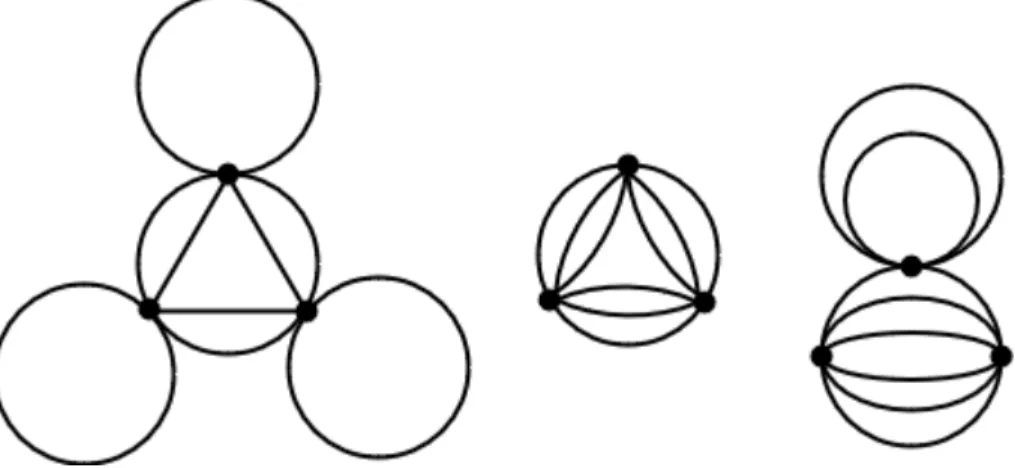
At order C3_{, we are evaluating three interactions, the expression of which}

takes the form

✏i✏j✏k✏l (pi1 pj1+qk2 ql2) (pi2 pj2+qk1 ql1) (pi3 pj3+qk3 ql3). (31)

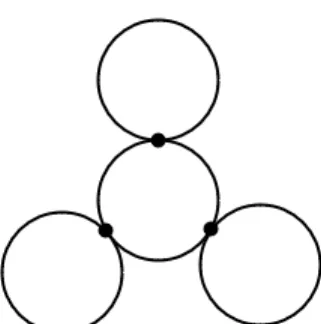
Each of which corresponds to the third order bubble diagrams.

Figure 5: One of four third order diagrams

Figure 7: The third of four third order diagrams

Figure 8: The last third order diagram

4.2

Three-Body Method

For three-body interactions the calculation starts with the uncontracted form, using Q222 again and w as the third momentum variable. Note that we now

have three sets of two Levi-Civita tensors, each set of order equal to the number of particles of that flavor. Q222 for example will have six second order tensors,

which takes the form,

✏i✏j✏k✏l✏m✏n (pi1 pj1) (qk1 ql1) (wm1 wn1) ⇥ (pi2 pj2) (qk2 ql2) (wm2 wn2).

(32)

Thus, we find C andC2_{by contracting one and two delta functions respectively:}

✏i✏j✏k✏l✏m✏n (pi1 pj1+qk1 ql1+wm1 wn1) ⇥ (pi2 pj2) (qk2 ql2) (wm2 wn2),

(33)

✏i✏j✏k✏l✏m✏n (pi1 pj1+qk1 ql1+wm1 wn1) ⇥ (pi2 pj2+qk2 ql2+wm2 wn2).

(34)

structures that resemble diagrams at each order. FORM is essentially comput-ing symmetry factors to these diagrams, but we will need to use more specific software to process our output.

Figure 9: Sample diagrams for order 1 and 2 (there are more for order 2)

5

Output Processing

The cost of using FORM is that we do lose out on some of the simplification methods in other symbolic languages. However, Mathematica even lacks meth-ods for simplifying terms resulting from the calculation. To address this situa-tion, a set of python codes was used using the networkx library. The group used the original code for processing the results for the two-body system. There are a number of obstacles in the way simply using the same code for three-bodies, so several significant modifications were made to handle the terms arising from contracting three delta functions in the epsilon tensor formula. The original code, written by Yaqi Hou and Dr. Joaqu´ın Drut was modified successfully to process this data.

There are three main phases to the code

• Use the graph theory library networkx to simplify the initial terms

• Act these terms on partition functions

• Convert result to products of single particle canonical partition functions

Somewhere between items two and three, for higher orders of C, we must deal with the interesting terms that result, like forQ222at orderC2, there are

the two terms

3F(p1+q1 q2)F(p1)F(q2)F(q1)Q100( )Q100( )

F(p1+q1+w1 q2 w1)F(p1)F(q2)F(q1)F(w1)F(w1).

(35)

Where for Fermi gasses,

F(p) =ep2/2m (36)

In the final calculation for bn we integrate these functions. In more detail,

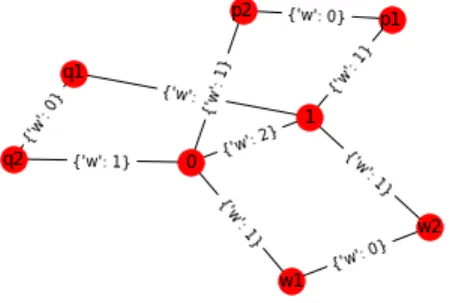
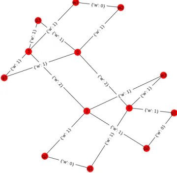
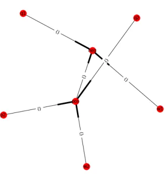
the code first reads in the results and removes redundant delta functions and merges identical terms by creating graphs for each delta function and checking for isomorphisms between graphs. A visual explanation follows in Figures 11, 12, and 13.

Last we have to process the more complex terms that arise at higher orders. At order C, one can write all Qin terms on the 1 particle partition function Q100. This is not the case at C2 or higher. To simplify these terms, we add

Figure 11: A six term delta graph, note the three nodes for each terms (terms with positive sign) going into the numbered node (referred to as a pseudonode) and three (negative sign terms) going into the other pseudonode. To help clarify, lines that connect nodes to nodes (2 term deltas) are given a weight ofw= 0, nodes to pseudonodes are given a weight ofw= 1 and pseudonode-pseudonode connections arew= 2

6

Results

We know immediately that b1 and b2 are 0 since there are no three-body

interactions with 1 or 2 particles. The rest require calculation using the recipes below.

Q1 b3= Q3 (37)

Q1 b4= Q4 b3Q21 (38)

Q1 b5= b2 b3Q21+ Q5

1 2 b3Q

3

1 b4Q21 (39)

Q1 b6= b3 b3Q21 b2Q21( b4+ b3Q1) + Q6 (40)

1 2 b3Q

4 1

1 2 b4Q

3

1 b5Q21 (41)

Q1 b7=

1

2b2 b3Q

4 1

1 2b

2

2 b3Q31 b3 b3Q31 b2 b4Q31 (42)

b4 b3Q21 b3 b4Q21 b2 b5Q21+ Q7 (43)

1 8 b3Q

5 1

1 2 b4Q

4 1

1 2 b5Q

3

1 b6Q21 (44)

Q1 b8=

1

2b2 b3Q

5 1

1 2b

2 2 b3Q41

1

2b3 b3Q

4 1

1

2b2 b4Q

4

1 (45)

b2b3 b3Q31 b4 b3Q31

1 2b

2

2 b4Q31 b3 b4Q31 (46)

b2 b5Q31 b5 b3Q21 b4 b4Q21 b3 b5Q21 b2 b6Q21+ (47)

Q8

1 8 b3Q

6 1

1 8 b4Q

5 1

1 2 b5Q

4 1

1 2 b6Q

3

1 b7Q21 (48)

The systematic cancellation of powers ofQ1are slightly more obvious now. We

now must insert the forms of three-body partition functions from Section 2.2. The full expressions become too large to large to print at higher orders. Data also exists for b9, but only the results up to order 5 will be discussed. The

remainder will be included in an upcoming publication by the group, as they still require sophisticated analysis methods to process the large outputs.

It is worth noting that the terms simplified by the directed graphs, appearing earlier as functionsF, can be evaluated using the process

Z 1

1

e 12P T

M P_dn_p=p_{det 2⇡M} 1 ₍₄₉₎

Additionally, in the remaining resulting partition function, the Gaussian integrals can be quickly performed to get results in any dimension using the equation

Q100(n ) =

Z 1

1

e n p2/2m_dD_{p (50)}

Which becomes in D dimensions

✓ _2⇡

mn

◆D/2

(51)

6.1

Q

Using the Q values calculated from an initial approximation, by performing dimensional analysis and removing all terms that do not scale like the volume squared, as present in b3, the following are obtained. These are likely only

valid as first order approximation in C as they agree with the groups calculation for up to b5, this will be investigated in the upcoming paper.

Q111=C

Q100( )2

3V2 (52)

Q211= C

Q100( )Q100(2 )

6V2 (53)

Q311=C

Q100( )Q100(3 )

9V2

Q221=CQ100(2 ) 2

12V2

(54)

Q411= CQ100( )Q100(4 )

12V2

Q321= C

Q100(2 )Q100(3 )

18V2

Q222= C Q100(2 ) 3

24V2_Q 100( )

(55)

Q511=C

Q100( )Q100(5 )

15V2

Q421=C

Q100(2 )Q100(4 )

24V2

Q322=C

Q100(2 )2Q100(3 )

36V2_Q 100( )

Q611= C

Q100( )Q100(6 )

18V2

Q521= CQ100(2 )Q100(5 )

30V2

Q431= C

Q100(3 )Q100(4 )

36V2

Q422=C

Q100(2 )2Q100(4 )

48V2_Q 100( )

Q332= C

Q100(2 )Q100(3 )2

54V2_Q 100( )

(57)

From the above we can find the general form of this approximation for QLM N

including the final division byQ1 as

( 1)L+M+N+1CQ100(L )Q100(M )Q100(N ) 3LM N Q100( )V2

(58)

6.2

b

in 1D

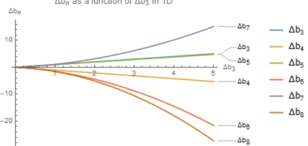
As mentioned earlier, up to b5 have been confirmed with other calculations

in the group for 1D (the dimension-general form will be given shortly). b3 is

used as a renormalizing parameter for ease of analysis. It is worth noting that while the analysis is consistent to b5 it is possible it diverges afterward. This

will be the subject of the upcoming paper, and will be investigated using more sophisticated methods, namely, automating the integration process for then partition functions using the matrix form in eq.49. In 1D, where ¯h=m=kB =

1, and using the dimensional approximation, the virial coefficients in 1D are

b1= 0 (59)

b2= 0 (60)

b3=C

"

2⇡

3

#

(61)

b4=

3 b3

2p2 (62)

b5=3

2

✓

1 4+

2 3p3

◆

b3 (63)

b6=3

2 0 @ 1 4 q 2 3 3 1 24p2

1

A b3 27

16

⇣_p

2 1⌘ b23 (64)

b7=

1 224

⇣

168 21p2 + 56p3 48p7⌘ b23+

b8= 9

4

✓

1 189

⇣

21p2 + 7p3 14p6 + 3p14⌘+

336p10 + 120p14 35 33 + 33p2 8p3 + 16p6 10080

!

b23+

3 2

0 @ 1

32

q

2 5

5

1 27p2

1 6p3

1 3p6

1 A b3

(66)

The dimension-general results, as confirmed by the group are

b4= 3

2

Q100(2 )

Q100 b3=

3

2d/2+1 b3 (67)

b5=

"

3Q2 100(2 )

Q100

+Q100(3 ) Q100

#

b3=

"

3 2d +

1 3d/2

#

b3 (68)

6.3

Plots

Figure 15: The virial coefficients as a function of b3

References

[1] E. Epelbaum, A. Nogga, W. Gl¨ockle, H. Kamada, Ulf-G. Meißner, and H. Witala. Three-nucleon forces from chiral e↵ective field theory. Phys. Rev. C, 66:064001, Dec 2002.

[2] Andr´e Heck. Form for pedestrians, Oct 2000.

[3] Maksim Kunitski, Stefan Zeller, J¨org Voigtsberger, Anton Kalinin, Lothar Ph. H. Schmidt, Markus Sch¨o✏er, Achim Czasch, Wieland Sch¨ollkopf, Robert E. Grisenti, Till Jahnke, D¨orte Blume, and Reinhard D¨orner. Obser-vation of the efimov state of the helium trimer. Science, 348(6234):551–555, 2015.

[4] B. A. Loiseau and Y. Nogami. Three-nucleon force. Nuclear Physics B, 2:470–478, August 1967.

[5] P. Mermod, J. Blomgren, B. Bergenwall, A. Hildebrand, C. Johansson, J. Klug, L. Nilsson, N. Olsson, M. ¨Osterlund, S. Pomp, U. Tippawan, O. Jon-sson, A. Prokofiev, P.-U. Renberg, P. Nadel-Turonski, Y. Maeda, H. Sakai, and A. Tamii. Search for three-body force e↵ects in neutron–deuteron scat-tering at 95 mev. Physics Letters B, 597(3):243 – 248, 2004.

[6] Scott E. Pollack, Daniel Dries, and Randall G. Hulet. Universality in three-and four-body bound states of ultracold atoms. Science, 326(5960):1683– 1685, 2009.

[7] A. J. Sarty. a Measurement of the Three-Body Photodisintegration of HELIUM-3 and its Relation to Three-Body Forces. PhD thesis, THE UNI-VERSITY OF SASKATCHEWAN (CANADA)., 1993.

[8] C. R. Shill and J. E. Drut. Virial coefficients of one-dimensional and two-dimensional fermi gases by stochastic methods and a semiclassical lattice approximation. Phys. Rev. A, 98:053615, Nov 2018.