Sharif University of Technology
Scientia IranicaTransactions E: Industrial Engineering http://scientiairanica.sharif.edu
Multi-stage investment planning and customer selection
in a two-echelon multi-period supply chain design
B. Abbasi, A. Mirzazadeh
, and M. Mohammadi
Department of Industrial Engineering, Faculty of Engineering, Kharazmi University, Tehran, Iran. Received 18 November 2017; received in revised form 15 January 2018; accepted 26 May 2018
KEYWORDS Supply Chain; Optimization; Metaheuristic; Reinvestment; Multi-stage
investment planning.
Abstract.In the supply chain of Fast-Moving Consumer Goods (FMCG), logistics costs represent a major part of total expenses. At these low-level chains, one usually faces a Vehicle Routing Problem (VRP). In practice, however, due to the high cost of service in many cases, some customers are not selected to serve. Investment-related restrictions in many cases make it impossible to serve some of the potential customers. In such conditions, designing a supply chain network, including a location-allocation problem in the warehouse, Multiple Depot Vehicle Routing Problem (MDVRP) at the distribution level, and customer selection at the retail level in several periods of time, is considered. In this respect, in addition to certain methods that can be used in small sizes, metaheuristic algorithms have been used to solve large-scale models. With the aim of improving the performance, if not improving a few diversications, algorithms are temporarily enhanced; eventually, by using statistical approaches, it has been demonstrated that this method could have a signicant impact on the quality of responses. Genetic Algorithm (GA) and Simulated Annealing (SA) algorithm have been used for this purpose.
© 2019 Sharif University of Technology. All rights reserved.
1. Introduction
In many supply chains, logistic costs comprise a major part of the total costs. This is also true for the supply chain of fast-moving consumer goods. At the low levels of these chains, one usually faces a VRP that increases the cost of logistic drastically, because production must be distributed among mainly small customers at greater distances. In practice, due to the high service cost in many cases, some clients are not chosen for serving. Restrictions associated with the investment in many cases make it impossible to serve some potential customers. With the advent of
*. Corresponding author.
E-mail addresses: behrooz.abbasi@Gmail.com (B. Abbasi); mirzazadeh@ khu.ac.ir (A. Mirzazadeh);
Mohammadi@khu.ac.ir (M. Mohammadi) doi: 10.24200/sci.2018.5608.1373
global businesses and the development of globalization, the administration of supply chains has drawn much attention. The high complexity of the underlying acquisition, production, and delivery means, as well as the growing number of parties included, further stresses the need for eective decision support methods. Two of the major concerns of all fast-moving consumer goods organizations include (a) decreasing the total expense of administering their supply chain and (b) improving their responsiveness, i.e., attempting to deliver the goods to retailers in the assured period [1]. In the current paper, a two-echelon model of the supply chain is considered. In its rst echelon, distribution warehouses are placed and, in the second echelon, customers are placed and distribution is done by designating vehicle routes. In addition, this model is able to select customers, meaning that the sale to a group of clients may not be aordable; therefore, there will not be any possibility to remove them. It is a common practice in distribution companies; they do
not consider themselves committed to serving all of the customers and, instead, protability indicators are the dened criteria for their decision-making. The model presented in this study considers several periods of time. Usually, demand change at dierent times causes problems in the form of multi-period to be modeled. In this study, however, in addition to changes in demand, nancial constraints constrain the possibility of investment and, as a result, the possibility of serving potential customers. Moreover, in this model, at the end of every month, the prot earned from the sales and distribution operations is reinvested in distribu-tion network development, and the development of infrastructures and vehicles is carried out; therefore, the number of customers increases gradually, too. Finally, potential customers for whom providing service is not cost-eective from an economic perspective are eliminated from the client list and do not receive any services. In models that have been developed for the supply chain network design, it is assumed that capital is required to start and develop a network, which may be limited or unlimited; however, in practice, multi-stage investment is conservative, and many industries, either in the medium or long run, are created over time. In this problem, designing a supply chain network is considered including a location-allocation problem in the warehouse, MDVRP at the distribution level, and customer's selection at the retail level in some period. Selection of the warehouses, allocation of customers to the stores, selection and deletion of some customers, determining the number of required vehicles and routing vehicles are done simultaneously and in several periods in the form of a model. In this model, the proceeds of the business of the company to develop a distribution network are invested and, in any given period, in accordance with the new investments, more customers are added to the distribution network. Table 1 presents a sample of a multi-stage investment process for a two-echelon supply chain with 10 potential customers in three time periods.
GAMS software is used in small sizes for problem-solving. Metaheuristic algorithms, including GA and SA, are used in problem-solving, and the obtained results are compared with each other.
In designing the algorithms, providing a new
operator and applying it to SA and GA algorithms led to the veriable improvement of the responses.
2. Literature review
2.1. Location-routing problem combined with the supply chain management
The location-routing problem is at focus in logistics administration domain where the main purpose is to determine the location and the number of facilities as well as the optimum route for the vehicles. Integrated location-routing models are used for solving the Facility Location Problems (FLP) and VRP, showing a good interaction between the above two decisions [2-5].
In addition to the combination of Location and VRP, researchers have also utilized other concepts in the supply chain management and production issues in a compound form with the VRP. Schmid et al. (2013) carried out a study on the problem of access to routing issues based on a supply chain management [6]. In this paper, the classic problem of routing vehicles from dierent directions has been discussed. It focuses on issues such as lot-sizing, timing, packaging, sorting, in-ventory, and constraints. Wang and Lee (2015) studied three-echelon and two-echelon supply chain networks with the aim of optimizing the prot. The current research investigates a capacitated facility location and assignment allocation issue of a multi-echelon supply chain in risky markets. In this study, the revised ant algorithm has improved the performance of the existing ant algorithms [7]. Dondo et al. (2011) modeled and solved a VRP with temporary warehouses in the supply chain management [8]. Osman and Mojahed (2016) studied the vehicle routing problem with capacitated transport vehicle routing restrictions on distribution to dierent suppliers [9]. Govindan et al. (2014) investigated the problem of two-echelon multi-vehicle route selection with time window to optimize the net-work of a sustainable supply chain in perishable foods. In the present research, the optimization model of the multi-function integrated sustainable objective in deciding the distribution in a supply chain of perishable food is studied. This issue is summarized in a two-echelon routing in a time window for supply chain network design and optimization of environmental and
Table 1. Illustration of a problem with 10 potential customers and two warehouses. Period of
time
Number of vehicles
Number of warehouses
Number of
customers Routes
1 1 1 4 W1!C2!C7!C4!C5!W1
2 2 1 6 W1!C2!C7 !C5!W1
W1!C3!C9!C4! W1
3 2 2 9 W1!C2!C7!C9!C1!C5!W1
economic objectives in a sustainable supply chain network [10]. Location Routing Inventory Problem with Transshipment (LRIP-T) is a collaboration of the three parts, including vehicle routing, location-allocation, and inventory management issues, in the supply chain that would facilitate the transshipment procedure in a way that the total system expense and the consumed time are decreased [11,1].
2.2. Metaheuristic algorithms in a supply chain optimization problem
Since supply chain optimization issues include NP-hard problems, many researchers have used metaheuristic al-gorithms to solve large-scale problems [2,12-14]. Setak et al. (2016) used SA and GA algorithms to overcome an issue of concurrent pickup and distribution with semi-soft time windows [12-14]. Wang et al. (2016) pro-posed an advanced cross-entropy algorithm for solving a closed-loop supply chain planning and compared the results of the problem-solving in the three algorithms of cross-entropy, GA, and advanced cross-entropy [15]. Hassanzadeh et al. (2016) used two algorithms for solving the problem of a bi-objective supply chain management issue in a ow-shop condition. The rst algorithm (HCMOPSO) is a multi-objective particle swarm optimization combined with a heuristic mu-tation operator, Gaussian membership function, and a chaotic sequence; the second algorithm (HBNSGA-II) is a non-dominated sorting genetic algorithm II with a heuristic criterion for the generation of initial population and a heuristic crossover operator [16]. Masoud and Mason (2016) developed a hybrid SA to overcome the automotive supply chain [17].
2.3. The main innovations
In summary, the set of existing innovations in this paper includes the following cases:
The possibility to deselect a client for economic reasons;
The possibility of the progressive development of the supply chain and distribution network;
Reinvestment of prot in expanding the network of supply chain and sales;
The possibility of customer selection, determining the warehouses, and determining the number of required vehicles and vehicle routing in a period of time, all at the same time;
Improving the performance of metaheuristic algo-rithms by considering two diversication rates and activating the second rate in case of no improved answer in several successive stages and its imple-mentation for the SA and GA algorithms.
3. Problem denition and modeling 3.1. Problem denition
In theoretical issues, it is generally assumed that necessary funds are available to develop the supply chain network and investment coherently. Once it is done in real terms, however, the investment may be made gradually and in several stages for various reasons. Lack of funds is one of the most signicant inuential parameters, and most of the designs created from revenues in the supply chain are funded. In such circumstances, infrastructure is developed, and the possibility of serving customers is facilitated.
This includes two levels of distribution: cen-ters/warehouses and customers/retailers. In the ware-house, it is required to select some distribution cen-ters/warehouses among several potential locations. Customers and vehicles are allocated to the ware-houses, too. At the level of customers/retailers, the problem involves choosing the path of service and determining the number of vehicles. Cases referred to in any period are investigated, and the amount of the investment includes the initial capital and prot from the sales in the previous periods. Figure 1 provides
a schematic illustration of a hypothetical answer to a problem with ten potential customers in three time periods. In the rst period (Figure 1(a)), a warehouse, an auto, and four customers are selected and allocated to the warehouse, and the direction of the movement of vehicles is specied. In the second period (Figure 1(b)), prots from the sale are allocated to buy a new vehicle, and two vehicles and a warehouse are selected. In addition, during this period, six customers are served, and the movement direction of two vehicles is provided. As can be seen, some of potential customers are eliminated due to economic reasons.
Many researchers have studied location-routing problems [18-20]. Since it has been determined that this problem is of NP-hard type [21], several algorithms are suggested to solve it precisely in small dimensions, and approximation algorithms are suggested for solving it in large dimensions [7,22-26]. Given that the issue in this article is a complex form of LRP, it is an NP-hard issue.
Assumptions
Available initial capital is determined;
Prot from each course can be invested in other short-term activities or used to develop the business of the company;
Short-term investments done from the prots of the business at the time of need can be invested in the activities related to the current business of the company;
The rate of capital return expected by shareholders is known and xed;
Every customer demand is known and xed;
The capacity of warehouses is unlimited;
The capacity of vehicles is specied and limited;
The maximum distance that a vehicle is passing is clear and limited, and it is the same for all vehicles;
The place of potential warehouses is clear;
To set up each warehouse, the company pays a certain fee;
The list and locations of potential customers are clear;
Each vehicle route starts from a warehouse and ends in the same warehouse;
Each customer is served exactly once by one of the autos.
Index sets
I Set of network nodes including customers and warehouses N Set of customers
M Set of warehouses
K Set of vehicles P Set of time periods
i; j; h The number of network nodes including the customer and the warehouse p The number of time periods k The number of vehicles Parameters and notations bigM A great number
cbip Customer demand i (i = 1; :::; N) in
terms of dollars in p period
qip Customer demand i (i = 1; :::; N) per
unit of weight in period p
wci The xed cost of setting up warehouse
i (i = N + 1; :::N + M) vck The expense of using vehicle k
c The xed expense of product displacement per km
dij The distance between nodes i and j
NT The maximum distance that a truck passes
Q The maximum capacity of the vehicle by weight
capital Initial capital available
int Acceptable rate of return of the investment
Decision variables
SCip If customer i is selected, it is 1;
otherwise, it is 0. (I = 1; :::; N) SWip If store i is selected, it is 1; otherwise,
it is 0. (I = N + 1; :::N + M) xijkp If from nodes i to j or vehicle k, a
move to be done is 1; otherwise, it is 0. AVkp If vehicle is selected k, it is 1; otherwise,
it is 0.
yi The auxiliary variable that is dened
to avoid creating the loop
capp The amount of capital available in
course p
invp Investments in period p
returnp Returning prot of period p
protp Net prot of period p
Z The net present value of investments (objective function)
Mathematical formulation
Objective and constraint functions of this issue are described, respectively, as follows:
max : z = inv1+ P
X
p=1
protp
subject to: N X i=1 K X k=1
xijkp= SCjp
(j = 1; :::; N + M; p = 1; :::; P ); (2)
N X j=1 K X k=1
xijkp= SCjp
(j = 1; :::; N + M; p = 1; :::; P ); (3)
N+MX i=1
xihkp N+MX
j=1
xhjkp= 0
(h = 1; :::; N + M; k = 1; :::; K; p = 1; :::; P ); (4)
N+MX i=1
N+MX j=1
xijkp bigM AVkp
(k = 1; :::; K; p = 1; :::; P ); (5)
N+MX i=1
N+MX j=1
dijxijkp NT
(k = 1; :::; K; p = 1; :::; P ); (6)
N X i=1 N X j=1
qijxijkp Q
(k = 1; :::; K; p = 1; :::; P ); (7)
K
X
k=1 N+MX
j=1
xijkp bigM SWip
(i=N +1; :::; N +M; p=1; :::; P ); (8) yi yj+ (M + N)xijkp N + M 1
(i=1; :::; N; j =1; :::; N; k =1; :::; K; p=1; :::; P ); (9) SCip SCip+1
(i = 1; :::; N; p = 1; :::; P 1); (10)
AVkp AVkp+1
(k = 1; :::; K; p = 1; :::; P 1); (11) SWip SWip+1
(i = N + 1; :::; N + M; p = 1; :::; P 1); (12)
invp= N+MX
i=N
W CiSWip+ K
X
k=1
V CkAVkp
(p = 1; :::; P ); (13)
returnp = N
X
i=1
cbiSCip c
0 @N+MX
i=1 N+MX j=1 K X k=1
dijxijkp
1 A
(p = 1; :::; P ); (14) capp= capp 1+ returnp
(p = 2; :::; P ); (15) cap1= capital + return1; (16)
inv1 capital; (17)
protp = returnp; (18)
protp = returnp+ invp invp+1
(p = 1; :::; P 1); (19)
N+MX j=1
xhjkp= N+MX
i=1
xihkp
(h=N +1; :::; N +K; k =1; :::; K; p=1; :::; P ); (20) xijkp= 0
(i = N + 1; :::; N + K; j = N + 1; :::; N + M; k = 1; :::; K; p = 1; :::; P ); (21) xijkp2 f0; 1g
(i = 1; :::; N + M; j = 1; :::; N + M; k = 1; :::; K; p = 1; :::; P ); (22) yi 0
(i = 1; :::; N); (23) capp 0
(p = 1; :::; P ); (24) invp 0
(p = 1; :::; P ); (25) returnp 0
SCip2 f0; 1g
(i = 1; :::; N; p = 1; :::; P ); (27) SWip2 f0; 1g
(i = 1; :::; N; p = 1; :::; P ); (28) AVkp2 f0; 1g
(k = 1; :::; K; p = 1; :::; P ); (29) xijkp2 f0; 1g
(i = 1; :::; N + M; j = 1; :::; N + M; k = 1; :::; K; p = 1; :::; P ): (30)
Eq. (1) shows the objective function of the prob-lem. In this issue, project cash ow declines in dierent time periods, and the resulting present value of money ow is evaluated. The objective function includes the cost of investment in the rst year, which has been shown to aect the cash ow negatively, and the prots of the business in future periods that are transferred to the rst year. To transfer the cash ow to the rst year, each ow is divided by (1+int)p. Constraints (2)
and (3) ensure that if a customer is elected, the client should be provided with service. These constraints also ensure that, in case of serving, this action is only to be done by a vehicle and in one visit. Constraint (4) states that if a vehicle enters a node, it will be out of the node, too. Constraint (5) ensures that if the xed fee of vehicles is not paid, it should not to be applied. Constraints (6) and (7) restrict the volume of vehicle load and the distance that the vehicle can move. Constraint (8) ensures that if the xed fee of the warehouses has not been paid, the inventory should not to be out of the store. Constraint (9) is used to eliminate the sub-tours between clients and storage [15,16]. Constraint (10) ensures that if customers are selected in a course and receive services, they should also receive services in later periods. Constraint (11) guarantees that if a vehicle is used once, it should also be operated later. Constraint (12) ensures that if a warehouse is used once, it should be active in the next period, too. Constraint (13) calculates the investment needed for each period. This investment includes the cost of setting up warehouses and applying vehicles. It should be noted that this amount calculates the total capital required, not the surplus capital required in that period. Constraint (14) computes the backward business prot of the company. Returning prots in each period include the revenue from sales and logistics costs, which have been negatively imported from the cash ow. Constraint (15) shows the amount of capital
available at the end of each period. This investment includes the capital available in the previous period and the returning prot in that period. It should be noted that this amount is calculated from the second period to the nal period. Constraint (16) calculates the amount of capital available at the end of the rst period. This investment includes the initial capital and prot returns of the rst period. Constraint (17) shows that the amount of investment in the rst period cannot exceed that of the initial capital. Constraint (18) shows the net income of the last period. Since no investment is done in this period, the total amount of the returned prot is considered as the net income. Constraint (19) shows the amount of net prot at the end of each period for the periods before the last period. This amount is equal to subtracting prots in each period and the amount of capital required for investment in the next period. The amount of the capital required is equal to the dierence between the amount of investment at the end of the next period and investment at the end of the current period. Constraint (20) ensures that every vehicle has moved from a warehouse and returned to that warehouse. Constraint (21) restricts the movements between the warehouses. Other constraints have identied zero and one variables as well as positive variables.
4. Solution algorithms
To overcome this problem, two metaheuristic rithms (GA and SA) are used. In each of these algo-rithms, the algorithm has been improved by applying changes. Therefore, if the answers do not improve in several periods, the diversication has increased. 4.1. Encoding and decoding
The coding system used in this paper is priority-based. Figure 2 presents a sample of this type of solution coding.
In this system, there are N customers and M storehouses when coding answers, and this coding produces M + N + 1 sequential digit randomly, whose sequence shows their service on the track. Moreover, numbers N + 1 to N + M are dedicated to the
storehouses. The customer's number, on the left side of each storage number left unallocated, will be allocated to this storage. The last number is also used as a separator. The number of stocks on the left side along with the clients assigned to the warehouse is selected, and other customers and stores are eliminated. For example, ten customers and two warehouses are shown in Figure 2. As is common practice in encoding this problem, 13 consecutive numbers have been used. Customers, stores, and separator numbers are marked as 1 to 10, 11-12, and 13, respectively. In this case, customers with numbers 5, 2, 6, 4 and Customers 9 are allocated to Stores 12 and 11, respectively, and Customers 3, 10, 1, 7 are eliminated and not served.
To allocate the vehicles, given that vehicles are of one kind, restrictions are used on the weight and distance of the vehicle. For this purpose, the allocation is initialized from the left side. In each allocation, the remaining weight of the truck and the distance needed to be passed are calculated. The return distance is also calculated, and if these numbers are able to cover the restrictions, the allocation is considered done; other-wise, the route is closed by calculating the distance of the returning vehicle, and another vehicle is deployed to the rest of route. This procedure continues untill achieving the total number of the warehouse. Upon arrival to each warehouse, the path is closed regardless of the remaining capacity of the vehicle. This process is repeated for all of the allocated warehouses.
A similar procedure is used to restrict the avail-able capital. To distribute the product, one storage is required at least, and a vehicle regarded as sucient initial capital is considered for it. As can be seen in Figure 2, in the rst round of Store 12, a lorry is considered as the initial investment. It is also assumed that because of weight restrictions and limitations on the distance passed by any vehicle, the possibility of providing service for only three customers exists. In addition, in this period, the route of a vehicle is set as 12, 5, 2, 6, and 12. In the second round, it is assumed that prots from sales to three customers in the rst round should only be provided using a new vehicle. An additional vehicle is used to serve Customer 4 in Routes 12, 4, and 12. As is specied, serving all customers requires the use of Warehouse 11, and the addition of at least one new vehicle, whose proceeds are assumed from the business in both pre-periods, fails to cover the required costs. Therefore, conditions have not changed in the third period, and four customers are served with a warehouse and two trucks. Finally, it is assumed that, in the fourth round, the possibility of using Warehouse 11 and adding one vehicle is provided; as a result, Routes 11, 9, 8 are added to the previous routes in the period.
For decoding the described code based on the method provided in the rst step, it is required to
determine the investment amount needed for service customers based on the order created for serving each customer. Algorithm 1 demonstrates this issue.
In addition, the instruction for calculating the objective function in Algorithm 2 is provided.
4.2. The genetic algorithm 4.2.1. Description of the algorithm
GA is a competitive evolutionary method that repeats the processes of the mechanism of natural selection and biological evolution [17,27]. This algorithm is designed on the principle that most adaptable organisms have a better chance of survival [28]. SA and GA include the most popular metaheuristic algorithms to solve large-sized problems or non-linear issues [29]. Genetic algorithms have been used by many researchers to solve problems of optimization of supply chain networks [30-33]. They are also used as combined with other algorithms by dierent researchers to solve optimiza-tion problems of supply chain [34-36,25]. A typical procedure of GA is illustrated in Figure 3 [37-40]. 4.2.2. Natural selection
In this study, tournament selection is used as natural selection. In this method, to select each parent, two answers are selected from the population, and the top option is selected as a parent.
4.2.3. GA operators Crossover operator
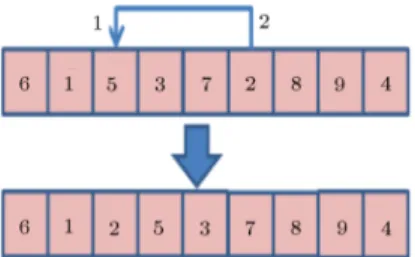
The crossover operator generates new responses based on the present responses. In this procedure, some of the features of parents' chromosomes are transmitted to children. In this article, the two-point operator is used for this purpose. Figure 4 shows an example of this operator.
Mutation operator
The mutation operator is designed and used to improve diversication in the genetic algorithm. In this paper, the shift-mutation operator is applied. Figure 5 shows the operator.
Two dierent mutation probabilities are used to improve the performance of this algorithm. The problem initiates with a mutation probability, and the answers improve based on GA. It is then expected that the process of achieving better solutions slows down, and the algorithm tends towards convergence. At this point, considering the output of the algorithm from possible local optimum points, if the responses are not improved within the specied number of generations, the second mutation probability is applied. This action increases diversication temporarily and leads to the production of new responses. With the rst improve-ment of the replies, the rate of the rst mutation prob-ability is activated again. It makes the algorithm have less chance of engagement in the local optimum points
Algorithm 1. Investment-calculating procedure.
Figure 3. The standard GA procedure.
Figure 4. A schematic of the two-point crossover operator.
Figure 5. An illustration of the shift mutation operator.
while maintaining its convergence. Another important point is that increasing the mutation probability can lead to an increase in calculations; as a result, the speed of the algorithm and the quality of the nal answer are reduced. Since two mutation probabilities are included in this algorithm, the initial mutation probability can
be reduced as much as possible. It also increases the speed of improving answers in early diversications.
Figure 6 compares the result of solving a problem using genetic algorithms with that of genetic algo-rithms with two mutation probabilities.
4.3. SA algorithm
4.3.1. Description of SA algorithm
SA is a metaheuristic algorithm used to overcome large-sized problems that have a large solution space and produce results close to the global optimum amount in a short amount of time. The SA algorithm was rst created by Metropolis et al. in 1953 to generalize the Monte Carlo method to determine the equations of state and, also, frozen states of n-body systems in the eld of metallurgy [3-5]. A typical procedure of SA is illustrated in Figure 7
4.3.2. Operators of SA algorithm Cooling scheme
In the cooling scheme, an exponential approach is used and, in each diversication, the temperature is multiplied in a xed number smaller than one. In this method, since there are only two temperatures in the algorithm, only one of the temperatures decreases and the other temperature is xed with the aim of
Figure 6. Comparison of the performances of GA and the two GAs in this paper.
Figure 7. The standard SA procedure.
increasing diversication in the whole process of solving the algorithm.
Acceptance probability
The possibility of selecting an inferior solution (Xnew)
is provided by the next equation, where Ti and Xi
are the temperature and the real solution amounts in iteration i.
p(Ti; Xnew; Xi) = exp(
Ti);
where = (f(Xnew) f(Xi)=f(Xi)) 100 is a
dimensionless parameter; it shows the relative rate of deviation of the perturbed solution (Xnew) from the
real one (Xi) [6].
Temperature settings
The temperature controls the diversication of the algorithm. In SA, the standard of temperature was
great at rst (diversication was high) and gradually decreased with the continuation of the solution. In this paper, two dierent SA algorithms are designed, and the results obtained by solving the problem using these two algorithms are compared with each other. In the rst algorithm, a standard SA is considered, and the initial temperature is determined according to the conventional methods of setting parameters. The second algorithm is designed with the aim of increasing diversication at times when the algorithm cannot improve the answer in several consecutive times. For this reason, two temperatures are considered in this algorithm. The rst temperature is reduced continuously based on the cooling scheme in dierent solving stages, and the chance of accepting bad answers and diversication reduces proportionately. If the algorithm is not able to improve the best answer
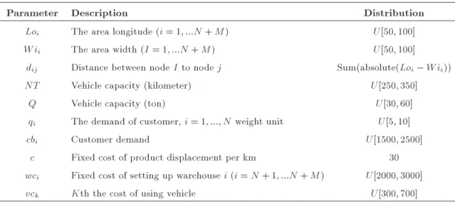
Table 2. Other statuses of the examined problems.
Parameter Description Distribution
Loi The area longitude (i = 1; :::N + M) U[50; 100]
W ii The area width (I = 1; :::N + M) U[50; 100]
dij Distance between node I to node j Sum(absolute(Loi W ii))
NT Vehicle capacity (kilometer) U[250; 350]
Q Vehicle capacity (ton) U[30; 60]
qi The demand of customer, i = 1; :::; N weight unit U[5; 10]
cbi Customer demand U[1500; 2500]
c Fixed cost of product displacement per km 30
wci Fixed cost of setting up warehouse i (i = N + 1; :::N + M) U[2000; 3000]
vck Kth the cost of using vehicle U[300; 700]
obtained during several periods (N), the second tem-perature is activated, which leads to the increase of the diversication algorithm. If the answer is improved, the rst temperature is activated again, and this process continues.
Termination condition
In this paper, since the ndings of the algorithms of the solution are compared with each other, the stoppage condition of the algorithms implies reaching a pre-specied time. This method facilitates the comparison of algorithms only through the investigation of the quality of their answers.
Producing vicinity answer
The shift operator that is introduced in Section 4.2.3 is used to produce the vicinity answer.
5. Numerical examples
To determine the performance of the algorithms, pro-ducing numerical examples is common [41]. In this section, the performance of the algorithms presented through numerical examples is shown. GAMS software is used for problem-solving in small sizes, and GA and SA are used for medium- and large-sized problems. The coding of metaheuristic algorithms is done by Matlab software.
5.1. Producing random responses
Two groups of random problems are used in this research. The rst group, containing 15 problems, includes small-scale numerical problems that have been used to verify the authenticity of the results of metaheuristic algorithms. The second group, which includes 21 medium- and large-scale problems, has been solved by metaheuristic algorithms, and responses are produced to assess the eectiveness of the changes
created by the algorithms. The algorithms are also compared with each other.
The parameters of numerical examples were pro-duced through the production of random data in MATLAB software. The method of producing the parameters of the problems is presented in Table 2.
5.2. Tuning the parameters of algorithms In this section, the set of parameters of the algorithms is considered. One of the common approaches in this regard is the use of numerical examples and Design of Experiments methods [7]. Central Composition Design (CCD) method is selected for this purpose, and MINITAB software is used for calculations. In this approach, ve levels are considered for each factor and, by considering the midpoints, the possibility of detecting the curve is provided. To provide numerical examples based on common methods, random numbers are generated. The production of numerical examples is described in Section 4.1. In this section, a mathe-matical model with 50 customers and ve warehouses is used, and the problem is solved in 20 time periods.
Normally, in GA, the parameters of mutation probability, the population size (pop) that ranges in [25 100] (Pm) in [0:1 0:4], and the maximum number of generations in various articles are intended to set the parameters [37,32]. Since the GA in this research is executed at a xed time, the number of generations deemed not necessary will be deleted from this group. Therefore, these two parameters have been consid-ered in GA. Regarding the GA with two mutation probabilities in addition to nPop, the two amounts intended for the mutation probability are [0.05 0.1] and [0:3; 0:5]. The parameter of the number of generations that reduces with non-improvement in response to mutation probability (N) in the range [4; 10] has been considered. The output of software in GA with two
Table 3. Coded coecients table (proposed GA).
Term Eect Coef. SE Coef. T -value P -value VIF
Constant 721061 4309 167.33 0.000
psize -15896 -7948 2327 -3.42 0.001 1.00
N 5612 2806 2327 1.21 0.232 1.00
MP 1 9346 4673 2327 2.01 0.048 1.00
MP 2 -2418 -1209 2327 -0.52 0.605 1.00
psizepsize -4767 -2384 2132 -1.12 0.267 1.03
NN 1090 545 2132 0.26 0.799 1.03
MP 1MP 1 -1823 -911 2132 -0.43 0.670 1.03
MP 2MP 2 -709 -354 2132 -0.17 0.868 1.03
psizeN -900 -450 2850 -0.16 0.875 1.00
psizeMP 1 -5567 -2784 2850 -0.98 0.332 1.00
psizeMP 2 1540 770 2850 0.27 0.788 1.00
NMP 1 14798 7399 2850 2.60 0.011 1.00
NMP 2 11828 5914 2850 2.07 0.041 1.00
MP 1MP 2 -8101 -4051 2850 -1.42 0.159 1.0
Figure 8. Optimization plot of the objective function (the proposed GA).
mutation probabilities is oered in Eq. (31):
Result = 742943+368 psize 11612 N +315838 MP 1 18282 MP 2 3:81 psizepsize + 61 NN
1458325 MP 1MP 1 15750 MP 2MP 2 6:0 psizeN 4454 psizeMP 1
+ 205 psizeMP 2 + 98653 NMP 1
+13142 NMP 2 1080167 MP 1MP 2: (31)
In Table 3, the testing hypothesis and the coecients of this problem are provided, and the output results of optimization of parameters of this algorithm are
provided in Figure 8. Accordingly, the size = 10, N = 13, MP 1 = 0:125, and MP 2 = 0:56 are considered. The output of analysis presented in the GA algorithm parameters in Eq. (32) is provided:
Result =779412 1578 psize 107645 MP + 5:04 psizepsize 145689 MPMP
+ 1868 psizeMP: (32)
The optimal parameter values of the algorithm are 40 upsize = and MP = 0:138. The optimization plot of the algorithm is presented in Figure 9.
In SA algorithm, two parameters of temperature [100 200] and the number of vicinity solutions created in each temperature It-num [30 50] to set the parame-ters have been considered. The method used to set the
Figure 9. Optimization plot of the objective function (GA).
Figure 10. Optimization plot of the objective function (SA).
parameters is similar to other algorithms. The result is provided in Eq. (33), and the optimization plot of this algorithm is presented in Figure 10.
Result =774039 500 temperature 1568 It-num + 2:11 temperaturetemperature
+ 18:4 It-numIt-num
+ 0:8 temperatureIt-num : (33)
On this basis, the optimum values are calculated as equal to 221 degrees for the temperature and equal to 54 for It-num. Regarding the SA algorithm considered in this article, two values are created for Temperature 1 [100 200] and Temperature 2 [150 300]. The number of vicinity solutions created in each degree It-num [30 50] and the number of successive answers are considered in case of failure to improve the optimal answer and the temperature range changes N [100 200]. The results of Eq. (34) and the optimization plot of this algorithm
are presented in Figure 11.
Result =653913 + 139 temp1 + 62 temp2
+ 3427 It-num 132 N+0:061 temp1temp1
0:378 temp2temp2 43:7 It-numIt-num
0:789 NN 0:505 temp1temp2
5:71 temp1It-num + 1:218 temp1N
+ 3:15 temp2It-num + 0:572 temp2N
+ 2:05 It-numN: (34)
On this basis, the optimal amounts of Temperature 1 and Temperature 2 are calculated as equal to 50 degrees and 375 degrees. It-num equals 53 and N equals 159. 5.3. Solving numerical problems in small sizes Model verication and validation have been among the concerns of researchers in the eld of mathematical
Figure 11. Optimization plot of the objective function (the proposed SA).
Table 4. The results of numerical examples for validation analysis. Test
problem
Number of customers
(N)
Number of warehouses
(M)
Number of periods
(P )
GAMS answer GA
Final solve
Best
possible Time
Final
solve Time
1 4 1 2 8350 9184 2.46 8350 5
2 4 1 4 17604 19363 43.84 17731 5
3 4 1 6 25483 27583 910.8 25483 5
4 5 2 1 4745 5164 2.53 4800 7
5 5 2 2 11786 12930 26.94 11891 7
6 5 2 3 18088 19897 98.31 18264 7
7 5 2 4 24007 26197 36.93 24197 7
8 6 2 1 4527 4972 14.62 4527 8
9 6 2 2 12140 13354 242.96 12140 8
10 6 2 3 19128 21106 1000.01 19128 8
11 6 2 4 25479 29274 1000.01 25480 8
12 7 3 1 8127 8939 75.51 8127 10
13 7 3 2 18243 19647 991.53 18243 10
14 7 3 3 27274 29865 208.76 27439 10
15 7 3 4 32734 38354 1000.03 35799 10
models [42-44]. Verication ensures that the concep-tual description and the solution of the pattern are em-ployed truly so that the real condition can be presented. In the validation process, the numerical simulation is associated with the experimental data, and the precision of the simulation is determined [45]. Simple examples, with predetermined answers, are used to investigate the verication of algorithms. The answer obtained from problem-solving is compared with the predetermined answers to investigate the verication of the model. The validity of algorithms is investigated through 15 numerical examples. For this purpose, 15 numerical examples with small dimensions are solved simultaneously using GAMS and metaheuristic
algo-rithms, and the results are compared with each other. Table 4 presents the outcomes of this analysis for GA and GAMS. It should be noted that the results of other algorithms used are similar to those obtained from the GA. The termination condition of solution algorithm through GAMS software is satised by achieving an optimal algorithm and an answer with a 10% dierence from that with high limits, or by the passage of 1000 seconds as of the time of solution. A number of nodes have been considered for solving the problem of time by metaheuristic algorithms. According to the results obtained and the minuscule dierence between them, the responses obtained from metaheuristic algorithms can be regarded as valid.
5.4. Solving numerical problems 5.4.1. Solving test problems
In this section, 21 problems in medium and large sizes are randomly generated and explained ve times by four algorithms and are resolved each time over a period of ninety (M + N). The values of the best answer and the average of 5 answers to the problem are extracted and compared with each other by statistical methods. Table 5 shows a summary of the results obtained in the two GAs. The results obtained by problem-solving by two SA algorithms are presented in Table 6. For this purpose, statistical analysis of the priority of the considered operator, a dierence of the best answers, and the average of answers generated by the two algorithms are calculated in each of the problems, and the test H0: 0 against H1: < 0 is tested for them through the t-statistic at a 5% level of signicance. The results obtained from two GA algorithms and SA considered by this article are deducted from each other, and the above test is done for them. MINITAB software is used for this purpose.
The results of software output are presented in Table 7. In this study, the following results were obtained:
At a 5% level of acceptance, the hypothesis of the higher best answer than the conventional GA produced by the GA considered in this paper is not rejected (P -value = 0.002);
At a 5% level of acceptance, the hypothesis of the higher best answer than the conventional GA produced by the GA considered in this paper is not rejected (P -value = 0.003);
At a 5% level of acceptance, the hypothesis of the higher best answer than the conventional GA produced by the GA considered in this paper is not rejected (P -value = 0.000);
At a 5% level of acceptance, the hypothesis of the higher best answer than the conventional GA produced by the GA considered in this paper is not rejected (P -value = 0.000);
At a 5% level of acceptance, the hypothesis of the higher best answer than the GA considered in this
Table 5. The results of numerical examples (GA and the proposed GA).
GA Proposed GA Deviation
(GA- proposed GA)
T P M N P Best Average Best Average Best Average
1 2 30 3 129600 125678 130550 125062 950 616
2 2 30 4 170830 164480 170200 164362 630 118
3 2 30 7 260050 252608 259430 254334 620 1726
4 3 40 3 143270 136614 139630 132200 3640 4414
5 3 40 5 229330 226904 233140 229062 3810 2158
6 3 40 10 394740 383708 398780 385316 4040 1608
7 4 50 5 303040 289144 292470 282152 10570 6992
8 4 50 10 507610 491236 499350 491952 8260 716
9 4 50 15 608510 604358 635390 614698 26880 10340
10 5 60 5 366010 352692 362380 357976 3630 5284
11 5 60 10 601020 596160 606600 596022 5580 138
12 5 60 15 744190 739688 773160 758496 28970 18808
13 5 70 5 448830 439790 453780 437584 4950 2206
14 5 70 10 741880 734660 752430 734950 10550 290
15 5 70 15 904670 896278 941040 919170 36370 22892
16 6 80 10 805780 794812 823440 817676 17660 22864
17 6 80 15 1012100 994820 1022900 1003120 10800 8300 18 6 80 20 1128200 1114440 1160500 1146180 32300 31740
19 6 90 10 902840 886194 908730 887288 5890 1094
20 6 90 15 1128600 1111980 1162200 1129400 33600 17420 21 6 90 20 1250800 1230700 1272100 1262440 21300 31740
Table 6. The results of numerical examples (SA).
SA Proposed SA Deviation
(SA- proposed GA)
T P M N P Best Average Best Average Best Average
1 2 30 3 129450 124488 129570 126064 120 1576
2 2 30 4 163110 160922 167580 162860 4470 1938
3 2 30 7 256890 253870 262880 258578 5990 4708
4 3 40 3 140230 133874 138600 130938 1630 2936
5 3 40 5 232290 222634 235180 226814 2890 4180
6 3 40 10 398420 391344 408660 398212 10240 6868
7 4 50 5 293040 284102 297360 293424 4320 9322
8 4 50 10 505200 499448 507380 501752 2180 2304
9 4 50 15 630700 623570 638270 632148 7570 8578
10 5 60 5 361040 351332 367140 360212 6100 8880
11 5 60 10 614960 603178 624260 613004 9300 9826
12 5 60 15 768820 757702 796400 785202 27580 27500
13 5 70 5 439890 430446 450740 446008 10850 15562
14 5 70 10 738460 730264 771690 750610 33230 20346
15 5 70 15 932820 927292 945900 933406 13080 6114
16 6 80 10 824400 806942 838360 829922 13960 22980
17 6 80 15 1029100 1016060 1061100 1039720 32000 23660 18 6 80 20 1172800 1158940 1197900 1183840 25100 24900
19 6 90 10 904450 892660 927530 907728 23080 15068
20 6 90 15 1130900 1124940 1171600 1147320 40700 22380 21 6 90 20 1268300 1260440 1310100 1296460 41800 36020
Table 7. The results of statistical analyses.
Test H0 H1 N Mean St Dev SE mean 95% upper
Boun T P
Best GA- proposed GA = 0 < 0 21 {10300 14408 3144 {4877 {3.28 0.002 Average GA- proposed GA = 0 < 0 21 {7738 11728 2559 {3324 {3.02 0.003 Best SA- proposed SA = 0 < 0 21 {14901 13513 2949 {9816 {5.05 0.000 Average SA- proposed SA = 0 < 0 21 {12846 10393 2268 {8935 {5.66 0.000
Best Proposed
GA-proposed SA = 0 < 0 21 {11905 13206 2882 {6935 {4.13 0.000
Average Proposed
GA-proposed SA = 0 < 0 21 {14037 12069 2634 {9495 {5.33 0.000
paper produced by the SA algorithm considered in this paper is not rejected (P -value = 0.000);
At a 5% level of acceptance, the hypothesis of the higher best answer than the SA considered in this paper produced by the SA algorithm considered in this paper is not rejected (P -value = 0.000).
The idea proposed to improve the performance of GA and SA algorithms managed to improve the
per-formance of both algorithms considerably. In addition, according to the statistical tests of the four algorithms investigated, the SA algorithm considered by this paper showed better performance than the other algorithms.
6. Conclusion and future research
In this problem, designing a supply chain network, including a location-allocation problem in the
ware-house, VRP in distribution, and customer selection at the retail level in some periods of time is considered. Selection of warehouses, allocation of customers to the warehouse, selection and deletion of some cus-tomers, determining the number of required vehicles and routing vehicles, is done simultaneously and in one period in the form of a model. In this model, the proceeds of the business of the company are invested to develop a distribution network and, in any period, more customers are added to the distribution network by the new investments. A coding system of responses is proposed to this problem, and the problem is solved through GAMS software and metaheuristic algorithms. Two algorithms of SA and GA are used for this purpose, and a number of ways are oered to improve them. Finally, it was shown that the results obtained by implementing these methods improved considerably. In GA, this change led to 1.2 percent and 1.6 percent improvement in the average of solutions and the best answer; in SA algorithm, this change led to 2.1% and 2.4% improvement in the average of solutions and the best answers.
In future researches of this problem, the number of levels can be increased or parameters such as demand can be certainly considered. Moreover, since the proposal of two existing diversications on both SA and GA algorithms could lead to improvement in the solutions, this idea can be applied to other algorithms.
References
1. Setak, M., Azizi, V., Karimi, H., and Jalili, S. \Pickup and delivery supply chain network with semi soft time windows: metaheuristic approach", International Journal of Management Science and Engineering Man-agement, 12(2), pp. 89-95 (2016).
2. Tavakkoli-Moghaddam, R., Gazanfari, M., Alinaghian, M., Salamatbakhsh, A., and Norouzi, N. \A new mathematical model for a competitive vehicle rout-ing problem with time windows solved by simulated annealing", Journal of Manufacturing Systems, 30(2), pp. 83-92 (2011).
3. Riquelme-Rodrguez, J.-P., Gamache, M., and Langevin, A. \Location arc routing problem with inventory constraints", Computers & Operations Re-search, 76, pp. 84-94 (2016).
4. Karaoglan, I., Altiparmak, F., Kara, I., and Dengiz, B. \The location-routing problem with simultaneous pickup and delivery: Formulations and a heuristic approach", Omega, 40(4), pp. 465-477 (2012).
5. Mehrjerdi, Y.Z. and Nadizadeh, A. \Using greedy clus-tering method to solve capacitated location-routing problem with fuzzy demands", European Journal of Operational Research, 22(1), pp. 75-84 (2013).
6. Schmid, V., Doerner, K.F., and Laporte, G. \Rich routing problems arising in supply chain
manage-ment", European Journal of Operational Research, 224(3), pp. 435-448 (2013).
7. Wang, K.-J. and Lee, C.-H. \A revised ant algorithm for solving location-allocation problem with risky de-mand in a multi-echelon supply chain network", Ap-plied Soft Computing, 32, pp. 311-321 (2015).
8. Dondo, R., Mendez, C.A., and Cerda, J. \The multi-echelon vehicle routing problem with cross docking in supply chain management", Computers & Chemical Engineering, 35(12), pp. 3002-3024 (2011).
9. Osman, S. and Mojahid, F. \Capacitated transport vehicle routing for joint distribution in supply chain networks", International Journal of Supply Chain Management, 5(1), pp. 25-32 (2016).
10. Govindan, K., Jafarian, A., Khodaverdi, R., and Devika, K. \Two-echelon multiple-vehicle location-routing problem with time windows for optimization of sustainable supply chain network of perishable food", International Journal of Production Economics, 152, pp. 9-28 (2014).
11. Shari, S.S.R., Omar, M., and Moin, N.H. \Location routing inventory problem with transshipment points using p-center", In Industrial Engineering, Manage-ment Science and Application (ICIMSA), 2016 Inter-national Conference on, IEEE (2016).
12. Schmid, V., Doerner, K.F., and Laporte, G. \Rich routing problems arising in supply chain manage-ment", European Journal of Operational Research, 224(3), pp. 435-448 (2013).
13. Chan, F.T., Jha, A., and Tiwari, M.K. \Bi-objective optimization of three echelon supply chain involving truck selection and loading using NSGA-II with heuris-tics algorithm", Applied Soft Computing, 38, pp. 978-987 (2016).
14. Ahmadi Javid, A. and Azad, N. \Incorporating loca-tion, routing and inventory decisions in supply chain network design", Transportation Research Part E., 46(5), pp. 582-597 (2010).
15. Wang, Z., Soleimani, H., Kannan, D., and Xu, L. \Advanced cross-entropy in closed-loop supply chain planning", Journal of Cleaner Production, 135, pp. 201-213 (2016).
16. Hassanzadeh, A., Rasti-Barzoki, M., and Khosroshahi, H. \Two new meta-heuristics for a bi-objective supply chain scheduling problem in ow-shop environment", Applied Soft Computing, 49, pp. 335-351 (2016).
17. Pasandideh, S.H.R., Niaki, S.T.A., and Asadi, K. \Bi-objective optimization of a multi-product multi-period three-echelon supply chain problem under uncertain environments: NSGA-II and NRGA", Information Sciences, 292, pp. 57-74 (2015).
18. Lopes, R.B., Ferreira, C., and Santos, B.S. \A simple and eective evolutionary algorithm for the capaci-tated location-routing problem", Computers & Opera-tions Research, 70, pp. 155-162 (2016).
19. Min, H., Jayaraman, V., and Srivastava, R. \Combined location-routing problems: A synthesis and future research directions", European Journal of Operational Research, 7(1), pp. 1-15 (1998).
20. Mokhtarinejad, M., Ahmadi, A., Karimi, B., and Rahmati, S.H.A. \A novel learning based approach for a new integrated location-routing and scheduling prob-lem within cross-docking considering direct shipment", Applied Soft Computing, 34, pp. 274-285 (2015).
21. Perl, J. and Daskin, M.S. \A warehouse location-routing problem", Transportation Research Part B: Methodological, 19(5), pp. 381-396 (1985).
22. Prins, C., Prodhon, C., Ruiz, A., Soriano, P., and Woler Calvo, R. \Solving the capacitated location-routing problem by a cooperative Lagrangean relaxation-granular tabu search heuristic", Transporta-tion Science, 41(4), pp. 470-483 (2007).
23. Vincent, F.Y., Lin, S.W., Lee, W., and Ting, C.J. \A simulated annealing heuristic for the capacitated location routing problem", Computers & Industrial Engineering, 58(2), pp. 288-299 (2010).
24. Escobar, J.W., Linfati, R., and Toth, P. \A two-phase hybrid heuristic algorithm for the capacitated location-routing problem", Computers & Operations Research, 40(1), pp. 70-79 (2013).
25. Syarif, A., Yun, Y., and Gen, M. \Study on multi-stage logistic chain network: a spanning tree-based genetic algorithm approach", Computers & Industrial Engineering, 43(1), pp. 299-314 (2002).
26. Hajiaghaei-Keshteli, M. \The allocation of customers to potential distribution centers in supply chain net-works: GA and AIA approaches", Applied Soft Com-puting, 11(2), pp. 2069-2078 (2011).
27. Michalewicz, Z. and Fogel, D.B., Summary, in How to Solve It: Modern Heuristics, Springer, pp. 483-494 (2004).
28. Bueno, P.M., Jino, M., and Wong, W.E. \Diversity ori-ented test data generation using metaheuristic search techniques", Information Sciences, 259, pp. 490-509 (2014).
29. Diabat, A. \Hybrid algorithm for a vendor managed inventory system in a two-echelon supply chain", Eu-ropean Journal of Operational Research, 238(1), pp. 114-121 (2014).
30. Costa, A., Celano, G., Fichera, S., and Trovato, E. \A new ecient encoding/decoding procedure for the design of a supply chain network with genetic algo-rithms", Computers & Industrial Engineering, 59(4), pp. 986-999 (2010).
31. Zegordi, S.H., Abadi, I.K., and Nia, M.B. \A novel genetic algorithm for solving production and trans-portation scheduling in a two-stage supply chain", Computers & Industrial Engineering, 58(3), pp. 373-381 (2010).
32. Kannan, G., Sasikumar, P., and Devika, K. \A genetic algorithm approach for solving a closed loop supply chain model: A case of battery recycling", Applied Mathematical Modelling, 34(3), pp. 655-670 (2010).
33. Yeh, W.-C. and Chuang, M.-C. \Using multi-objective genetic algorithm for partner selection in green supply chain problems", Expert Systems with Applications, 38(4), pp. 4244-4253 (2011).
34. Jamshidi, R., Ghomi, S.F., and Karimi, B. \Flexible supply chain optimization with controllable lead time and shipping option", Applied Soft Computing, 30(5), pp. 26-35 (2015).
35. Assarzadegan, P. and Rasti-Barzoki, M. \Minimizing sum of the due date assignment costs, maximum tardiness and distribution costs in a supply chain scheduling problem", Applied Soft Computing, 47, pp. 343-356 (2016).
36. Masoud, S.A. and Mason, S.J. \Integrated cost op-timization in a two-stage, automotive supply chain", Computers & Operations Research, 67, pp. 1-11 (2016).
37. Fahimnia, B., Davarzani, H., and Eshragh, A. \Plan-ning of complex supply chains: A performance compar-ison of three meta-heuristic algorithms", Computers & Operations Research, 89, pp. 241-252 (2018).
38. Dai, Z. and Zheng, X. \Design of close-loop supply chain network under uncertainty using hybrid genetic algorithm: A fuzzy and chance-constrained program-ming model", Computers & Industrial Engineering, 88, pp. 444-457 (2015).
39. Pasandideh, S.H.R., Niaki, S.T.A., and Nia, A.R. \A genetic algorithm for vendor managed inventory control system of multi-product multi-constraint eco-nomic order quantity model", Expert Systems with Applications, 38(3), pp. 2708-2716 (2011).
40. Soleimani, H., Seyyed-Esfahani, M., and Shirazi, M.A. \Designing and planning a multi-echelon multi-period multi-product closed-loop supply chain utilizing ge-netic algorithm", The International Journal of Ad-vanced Manufacturing Technology, 68(1-4), pp. 917-931 (2013).
41. Ozkr, V. and Baslgil, H. \Multi-objective optimiza- tion of closed-loop supply chains in uncertain environ-ment", Journal of Cleaner Production, 41, pp. 114-125 (2013).
42. Haridass, K., Valenzuela, J., Yucekaya, A.D., and Mc-Donald, T. \Scheduling a log transport system using simulated annealing", Information Sciences, 264, pp. 302-316 (2014).
43. Subramanian, P., Ramkumar, N., Narendran, T.T., and Ganesh, K. \PRISM: PRIority based SiMulated annealing for a closed loop supply chain network design problem", Applied Soft Computing, 13(2), pp. 1121-1135 (2013).
44. Tognetti, A., Grosse-Ruyken, P.T., and Wagner, S.M. \Green supply chain network optimization and the
trade-o between environmental and economic objec-tives", International Journal of Production Economics, 170, pp. 385-392 (2015).
45. Oberkampf, W.L., Trucano, T.G., and Hirsch, C. \Verication, validation, and predictive capability in computational engineering and physics", Applied Me-chanics Reviews, 5(7), pp. 345-384 (2004).
Biographies
Behrouz Abbasi is a PhD student of Industrial Engineering at the Kharazmi University in Iran. He earned MD and BS in Industrial Engineering in 2005 and 2001, respectively. His research and teaching interests are supply chain, combinatorial optimization, inventory optimization, excellence models, strategy formulation, and balanced scorecard.
Aboulfazl Mirzazadeh is a Professor of Industrial Engineering at Kharazmi University, Tehran, Iran. His research areas are uncertain decision-making, produc-tion/inventory control, supply and operations
man-agement, and quality management tools. He has more than 80 published papers in high-quality journals and more than 55 international conference papers. He is now the Editor-in-Chief of IJSOM and, also, the Scientic Committee manager of the International Conference. He earned several awards as the best researcher, best faculty member in the international collaborations, and best lecturer. In addition, he is a member of Journal's Editorial Board, Conferences Scientic Committee, and International Associations. Mohammad Mohammadi is an Associate Professor at the Department of Industrial Engineering at the Kharazmi University, Tehran, Iran. He received his BS degree in Industrial Engineering from Iran University of Science and Technology, Tehran, Iran in 2000, and his MS and PhD degrees in Industrial Engineering from Amirkabir University of Technology, Tehran, Iran in 2002 and 2009, respectively. His research and teaching interests include applied operations research, sequencing and scheduling, production planning, time series, metaheuristics, and supply chains.