Presenting a three-objective model in location-allocation problems using combinational interval full-ranking and maximal covering with backup model

Presenting a three-objective model in location-allocation problems

using combinational interval full-ranking and maximal covering

with backup model

Majedeh Kordjazi

_{, Abolfazl Kazemi}

1

Faculty of Industrial and Mechanical Engineering, Qazvin Branch, Islamic Azad University, Qazvin, Iran

[email protected], [email protected]

Abstract

Covering models have many applications in a wide variety of real-world problems. But some assumptions of covering models are not realistic enough. Accordingly, a general approach would not be able to answer the needs of encountering varied aspects of real-world considerations. Assumptions like the unavailability of servers, uncertainty, and evaluating more factors at the same time, are assumptions with which covering models are always faced; however, these models are not able to find any answers for them. Therefore, how to deal with these sorts of assumptions has been always a question. In this research, for facing unavailability and uncertainty in input data, backup covering and interval full-ranking models are addressed, respectively. Furthermore, by combining backup covering and interval full-ranking models (also conceptions), not only time is saved and more factors like efficiency and cost are simultaneously evaluated, but also covering considerations will be reachable in real aspects.

The proposed model in this paper is searching for three assumptions to cover major features. Emergency services are harshly sensible to delay, so the problem of server’s unavailability should be solved by considering backup coverage. Moreover, inefficient facilities were absolutely neglected in covering literature despite their destructive role in serving customer demands. To overcome this problem, we have entered efficiency to our model by considering location of each facility as an input for a revised version of data envelopment analysis which is called full-ranking model. As many research have proved to believe in uncertainty, no one can neglect this feature in real-world, we have just defined data in intervals to consider this feature. In final, the evident absence of research in three mentioned key features in one frame has left covering literature in defect and brought about the proposed three-objective model in this paper which is called combined maximal covering with backup model (MCBM) and interval full-ranking.

Keywords:

*Corresponding author.

ISSN: 1735-8272, Copyright c 2016 JISE. All rights reserved

Journal of Industrial and Systems Engineering

Vol. 9, special issue on location allocation and hub modeling, pp 53-70

Winter (February) 2016

1- Introduction

Hakimi (1965) for the first time introduced the concept of covering model and considered a vertex-covering model in a graph. He assigned the same weights to all the branches of this graph. Toregas et al. (1971) defined set covering problems (SCP), which aimed to determine the minimum number of servers (and their locations) which was required for covering all demand nodes. Church and Revelle (1974) noted the fact that, in many practical applications, allocated resources are not sufficient for covering all the existing facilities with the desired level of coverage. Assumptions of set covering models were extended by Daskin and Stern (1981) who then introduced multi-coverage concept. In their proposed model, backup coverage was considered; but, one of the primary issues of this model was unbalanced distribution of services.

Backup coverage was defined by Hogan and Revelle (1986) as a case, in which an extra facility was able to cover a demand node. They could overcome the issue of unbalanced distribution of services through maximizing backup coverage. Also, Revelle and Hogan (1989) replaced deterministic parameters in set covering problem with probabilistic parameters and thus included uncertainty conception in their model. Pirkul and Schilling (1989) presented a model, in which each new facility was capacitated and primary and backup services were provided to each demand node.

Kolen and Tamir (1990) concentrated on the uncapacitated versions of the covering problems. Although, in most of the real-world applications of covering problems, considering capacitated facilities is more realistic, this model was important because of its different attitude toward cost functions. Daskin (1995) focused on the variants of the set covering location model in his book; and included secondary objectives that were important in the facility location. Owen and Daskin (1998) assumed that all the demand nodes were not similar and then presented an uncapacitated version of set covering problem.

Thomas et al. (2002) included data envelopment analysis (DEA) in location-allocation models. First, they solved location-allocation model and then considered the optimum location of facilities as input data in data envelopment analysis. Lannoni and Morabito (2007) considered a multi-dispatch model, in which emergency demands were assumed to be different kinds and servers were distinctive. Baron et al. (2009) developed a set covering problem for the general class of location problems with stochastic demand and congestion (LPSDC). Berman et al. (2009) considered a covering problem, in which covering radius was a variable, and attempted to find the optimum radii beside the number and location of facilities.

Erdemir et al. (2010) proposed two models for locating aero-medical and ground ambulance service which were based on SCP and maximal covering location problem (MCLP). They also defined coverage as a combination of both response time and total service time. Lee and Lee (2010) introduced hierarchical covering location model, in which if distance from demand node i to facility was less than a given threshold, node i was fully covered. On the other hand, if the distance was beyond the pre-specified range, it was partially covered.

Berman and Wang (2011) developed a gradual covering location model, in which the weights of demand nodes on a network were random variables following an unknown distribution. Wen and Kang (2011) presented several optimum models in location-allocation with random stochastic demands. Afterward, they combined simplex algorithm, genetic algorithm, and random fuzzy simulation to present a hybrid intelligent algorithm. Moheb-alizade et al. (2011) included DEA in location-allocation models as the second objective for evaluating the efficiency of facilities in potential sites. They then presented a solving process based on the revised fuzzy parametric programming and minimum deviation method.

Applications and solutions of different proposed models in the covering literature were considered by Zanjirani et al. (2012). Their paper was also rich in terms of future research. Ni (2012) evaluated vertex-covering and arc-vertex-covering models in a network in a random environment. Shieh (2013) presented a new algorithm for solving covering models, which was able to solve fuzzy equations. Zarandi et al. (2013) focused on the dynamic aspects of covering models by infracting the assumption of single-period demands. Vidyarthi and Jayaswal (2014) considered the assumptions of immobile servers, stochastic demands and congestions simultaneously. Their model aimed at minimizing total cost by locating facilities, equipping them with appropriate capacities and allocating user demands to facilities, but it didn’t address unavailability of servers. Hosseininezhad et al. (2014) presented continuous capacitated covering model as

risk management model and defined demands as fuzzy numbers. Their model took uncertainty to account but forgot about efficiency and unavailability in comparison with our proposed model. Martinez-Salazar et al (2014) presented a combinational location routing problem in order to reduce distribution cost and keep balance of workloads for drivers. This study was rich in evaluating the efficiency of solution methods by considering both local search and evolutionary approaches but unavailability and uncertainty were neglected.

Ghodratnama et al (2015) considered a multi-objective hub location-allocation problem with a supply chain overview in order to minimize transportation and installation cost. However, they addressed uncertainty by defining fuzzy parameters; unavailability and uncertainty were not mentioned. Pereira et al (2015) contributed to covering literature in terms of solution method. They proposed a hybrid algorithm which combined a meta-heuristic and an exact method to solve a probabilistic maximal covering problem. As they focused on solution method, many assumptions like unavailability had been left unconsidered. As revealed by literature review, covering models have been subject of abundant studies but their wide variety doesn’t let researchers rely on a general approach to find a rational response for real-world problems. Accordingly, a practical approach would be taking all detailed characteristics to account and generalizing limited boundaries of classic models freely to include response to real-world challenges which are threatening us. A simple search in covering scope demonstrates that every model sets a framework for itself based on its target considerations. In this paper, we have focused on three fundamental features through which we can assure serving emergency services.

The proposed model in this paper is searching for three assumptions to cover major features. Emergency services are harshly sensible to delay, so the problem of server’s unavailability should be solved by considering backup coverage. Moreover, inefficient facilities were absolutely neglected in covering literature despite their destructive role in serving customer demands. To overcome this problem, we have entered efficiency to our model by considering location of each facility as an input for a revised version of data envelopment analysis which is called full-ranking model. As many research have proved to believe in uncertainty, no one can neglect this feature in real-world, we have just defined data in intervals to consider this feature. In final, the evident absence of research in three mentioned key features in one frame has left covering literature in defect and brought about the proposed three-objective model in this paper which is called combined maximal covering with backup model (MCBM) and interval full-ranking.

As we mentioned briefly, this model will be applicable in every condition which calls for emergency services such as hospitals in which serving demands should be performed as soon as possible, or else, serious issues will occur. This serious issue can differ from losing customers in private companies to leading someone to death in health centers.

The remaining of the paper is as follows: Section 2 defines interval full-ranking, MCBM, and combined MCBM and interval full-ranking model, respectively. In section 3, solution methods and parameter tuning are presented. Section 4 addresses the results and finally section 5 is devoted to conclusions and future works.

2- Problem definition

In this section, after focusing on interval full-ranking and MCBM models more precisely, a three-objective combinational model is proposed. Sets, parameters, and variables are also defined.

2-1- Introducing interval full-ranking model

Data envelopment analysis (DEA) is a mathematical programming used for determining the relative efficiency of decision making units (DMU), each one of which consumes multiple inputs for providing multiple outputs. The approach that estimates the efficiency of each DMU is the maximization of the ratio of weighted outputs to weighted inputs. Consider that n DMUs, each one consuming w inputs (i=1,2,…..w), should be evaluated in order to produce s outputs (o=1,2,…..s), and then measure the efficiency of DMUj

Max Z_p=∑s_o=1u_oB_op (1)

∑o=1s uoBoj-∑i=1w viDij≤ 0 j=1,2,……,n (2)

∑wi=1viDip =1 (3)

u_o, v_i ≥ ε (4)

where DMUp denotes the evaluated DMU, the decision variables are weight vectors u_o and v_i, D_oj and B_ij

are the input and output vectors for DMUj,and ε is a non-Archimedean infinitesimal equal to 0.0000001.

The objective value Z_p* denotes the relative efficiency of DMUp; if Z_p* =1, the efficiency of unit p will be 1

and this unit will be placed on an efficient frontier. However, if Z_p* <1, the efficiency of unit p will be less than 1 and this unit will not be placed on an efficient frontier (Sohrabi Haghighat and Khorram, 2005). Although classic models like model (1) proposes a suitable method for evaluating the efficiency of units, they are not always able to completely rank the units. In order to overcome this deficiency, interval full-ranking model is used. The main difference of this model and classic models is that the obtained weights for the inputs and outputs of each unit would be multiplied by the inputs and outputs of other units. Thus, they would provide a criterion for full-ranking in addition to be used for measuring weighted ratio of outputs to inputs (efficiency).

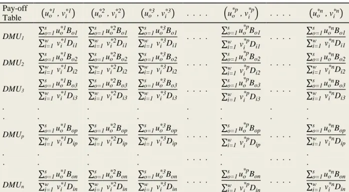
In the second step, all the criteria are placed in a pay-off table, in which every row displayed a rank for the related DMU. The digit which is obtained by the sum of all the criteria placed in each row is not a representative of the amount of efficiency; but, it provides full-ranking for units. The mathematical form of this interval full-ranking model is like model (1). After solving this model, optimum weights of inputs and outputs are obtained for DMUp as u_o*pand v_i*p and then the efficiency of DMUp is measured using Eq. (5):

Z_p* =∑ uo

*p Bop s o=1

∑wi=1v_i*pDip

(5)

After solving full-ranking model for all DMUs, optimum weights of each unit is multiplied by the inputs and outputs of other units based on Table 1 and Eq. (5), providing a criterion for full-ranking. Considering these conceptions, pay-off table would be as follows:

Table 1-Pay-off table

�u_o*n , v_i*n�

. . . .

�u_o*p , v_i*p�

. . . .

�u_o*3 , v_i*3� �u_o*2 , v_i*2�

�u_o*1 , v_i*1�

Pay-off Table

∑so=1uo*nBo1

∑wi=1 v_i*nDi1

. . . .

∑s_o=1u_o*pB_o1 ∑wi=1 v_i*pDi1

. . . .

∑so=1uo*3Bo1

∑wi=1 v_i*3Di1

∑so=1uo*2Bo1

∑wi=1 v_i*2Di1

∑so=1uo*1Bo1

∑wi=1 v_i*1Di1

DMU1

∑s_o=1u_o*nB_o2 ∑w_i=1 v_i*nD_i2

. . . .

∑so=1u_o*pBo2

∑w_i=1 v_i*pD_i2

. . . .

∑s_o=1u_o*3B_o2 ∑w_i=1 v_i*3D_i2 ∑s_o=1u_o*2B_o2

∑w_i=1 v_i*2D_i2 ∑s_o=1u_o*1B_o2

∑w_i=1 v_i*1D_i2 DMU2

∑so=1uo*nBo3

∑wi=1 v_i*nDi3

. . . .

∑s_o=1u_o*pB_o3 ∑w_i=1 v_i*pD_i3

. . . .

∑so=1uo*3Bo3

∑wi=1 v_i*3Di3

∑so=1uo*2Bo3

∑wi=1 v_i*2Di3

∑so=1uo*1Bo3

∑wi=1 v_i*1Di3

DMU3 . . . . . . . . . . . . . . . .

∑so=1uo*nBop

∑wi=1 v_i*nDip

. . . .

∑so=1u_o*pBop

∑w_i=1 v_i*pD_ip

. . . .

∑so=1uo*3Bop

∑wi=1 v_i*3Dip

∑so=1uo*2Bop

∑wi=1 v_i*2Dip

∑so=1uo*1Bop

∑wi=1 v_i*1Dip

DMUp . . . . . . . . . . . . . . . . . . . .

∑so=1uo*nBon

∑w_i=1 v_i*nD_in

. . . .

∑s_o=1u_o*pB_on ∑w_i=1 v_i*pD_in

. . . .

∑so=1uo*3Bon

∑w_i=1 v_i*3D_in ∑so=1uo*2Bon

∑w_i=1 v_i*2D_in ∑so=1uo*1Bon

∑w_i=1 v_i*1D_in DMUn

Elements that are placed on the main diameter of Table 1, display the efficiency amount of units. According to this table, the general equation could be extracted for ranking the criteria of DMUn as follows.

The more the criterion introduced in Eq. (6), the earlier priority the related unit would be.

θn=

∑so=1uo*1Bop

∑wi=1 v_i*1Dip

+∑so=1uo*1Bon

∑wi=1 v_i*1Din

+∑so=1uo*3Bon

∑wi=1 v_i*3Din

+…+∑ uo *p

Bon s o=1

∑wi=1 v_i*pDin

+…+∑so=1uo*nBon

∑wi=1 v_i*nDin

(6)

Due to the existence of uncertainty, DEA sometimes encounters uncertain data. Considering lack of research in this area, evaluating the efficiency of DMUs in a fuzzy or interval environment is of great importance; so, in this paper, the available level of resources in each of the candidate sites is assumed to be equal for all facilities, while the amount of these resources used by each facility are assumed to be variable. On the other hand, input and output data are assumed to be placed within the bounded intervals, in which lower bound showed the worst and upper bound indicated the best estimated amount thus far (Sohrabi Haghighat and Khorram, 2005).

D_ij∈�D_ijl ,D_iju� , B_oj∈�B_ojl ,B_oju� (7)

In Eq. (7), 𝐵𝐵_{𝑜𝑜𝑜𝑜}𝑙𝑙 is the lowest bound of output o for DMUj, B_oju is the upper bound of output o for DMUj

(o=1,2,…..s), Dijl is the lower bound of input i for DMUj, D_iju is the upper bound of input i for DMUj

(i=1,2,…..w), which are parameters of model, u_o is the weight attached to output o, and v_i is the weight attached to input i. Generally, intervals B and D can be written as follows:

D_ij=D

ij l_{+ ƛ}

ij�Dij u_-D

ij l_{�, B}

oj=Bojl + ƛʹ_oj�Boju-Bojl �, 0≤ ƛ_ij ,ƛʹ_oj≤1 (8)

By inserting Boj and Dij mentioned in Eq. (8) in Constraints (1) and (4) respectively, Constraints (9)-(12)

Max∑so=1 uo Bopl +∑o=1s uo ƛʹ_op�Buop-Bopl � (9)

𝒔𝒔.𝒕𝒕:∑w_i=1 v_i D_ipl +∑w_i=1p_ip�Du_ip-Dl_ip�=1 (10)

∑so=1uo Bojl +∑so=1 uo ƛʹ_oj �Boju-Bojl �-∑i=1w vi Dijl -∑i=1w vi ƛ_ij�Diju-Dijl�≤0 j=1,2,……,n (11)

u_o, v_i ≥ ε , 0≤ƛ_ij ,ƛʹ_oj≤1 (12)

A linear model would be achieved after variable transformation (13):

uoƛʹ_op=pʹ_op , viƛ_ip=p _ip , uoƛʹ_oj=pʹ_oj , viƛ_ij=p_ij (13)

After variable transformation (13), Constraints (9)-(11) will be change into Constraints (14)-(16):

Max∑o=1s uo Bopl +∑so=1pʹ_op�Buop-Blop� (14)

s. t:∑w_i=1 v_i D_ipl +∑w_i=1p_ip�D_ipu-Dl_ip�=1 (15)

∑so=1uo Bojl +∑ 𝑝𝑝ʹoj s

o=1 �Boju-Bojl �-∑wi=1vi Dijl -∑ pij w

i=1 �Diju-Dijl�≤0 j=1,2,…,n (16)

Considering Constraint (12) and variable transformation (13), the following could be written:

0≤ ƛʹ_oj≤1 , uo≥ ε → 0≤u_oƛʹ_oj=pʹoj≤uo 0≤ ƛ_ij≤1 , vi≥ ε → 0≤v_iƛ_ij=pij≤vi

After variable transformation (17), Constraint (12) would be eliminated from model (9) and Constraint (18) will be added to this model:

pʹ_oj≤uo p_ij≤vi pʹ_oj, p_ij≥0

After solving model (9), p'_op* , p_ip * , uo* , vi* can be obtained. By putting these values in objective function

(14), the optimum efficiency for DMUpis measured as follows:

Z*p=∑o=1s u*oBopl +∑so=1pʹ*_op�Bopu -Bopl � (19)

Therefore, by solving model (14), the first step in interval full-ranking model would be taken. Also, by combining Eq. (5) and (19), Eq. (20) is created to measure optimum efficiency of units:

Zp*=

∑s_o=1u_o*pBopl +∑ pʹop * s

o=1 �Bopu-Bopl �

∑wi=1 v*p_i Dipl+∑wi=1p*ip(Duip-Dipl)

₍₂₀₎

After solving model (14) for all DMUs, Eq. (6) and (20) led to a ranking criterion for DMUn which is measured by Eq. (21):

θDMUn=

∑so=1uo*1Bonl +∑ pʹo1 * s

o=1 �Bonu -Bonl �

∑wi=1 v*1_i Dinl+∑wi=1pi1*�Duin-Dinl�

+…+∑ uo

*n s

o=1 Bonl +∑ pʹon * s

o=1 �Bonu-Bonl �

∑wi=1 v*n_i Dinl+∑wi=1p*in(Duin-Dinl)

(21)

Similar to full-ranking model in crisp case, the unit with the highest index would rank first.

(18) (17)

2-2- Introducing maximal covering with backup model (MCBM)

One of the most popular facility location models is covering problem. Although covering models are not new, they have always been very attractive in terms of research, owing to their applicability in real-world life. Sometimes, covering models include emergency services like responding to serious trauma victims. In this case, responding to and covering demand nodes as soon as possible are highly important. To that end, Erdemir et al. (2010) proposed a model for locating aero-medical ambulance service, ground ambulance service, and transfer points simultaneously which responded to serious trauma victims.

In this model, coverage is defined as the combination of both response time and total service time and three types of it were considered: (i) Ground emergency medical service coverage, (ii) Air emergency medical service coverage, and (iii) Joint coverage of ground and air emergency medical service through transfer point, as a new conception in covering models.

These three types, led to three different coverage definitions, respectively. A trauma incident location is covered if and only if:

• Ground covered: if at least one ground ambulance is located within a pre-specified travel time to the incident location and it can take the trauma victim to the closest trauma center (TC) within a pre-specified time t by ground, or

• Air covered: at least one air ambulance is located within a pre-specified travel time to the incident location and it can take the patient to the closest TC within a pre-specified time t by air if the air ambulance is able to land onto the incident location, or

• Joint ground-air covered: if at least one ground ambulance-transfer point-air ambulance combination is located within a pre-specified travel time to the incident location, in such a way that the servers can take the patient to the closest TC within a pre-specified time t. This coverage option applies when the air ambulance cannot land at the crash scene. The ground ambulance takes the patient to a transfer point where it is met by an air ambulance. The patient is transferred and the air ambulance takes the patient to the TC (Erdemir et al., 2010).

Many factors influence the type of transportation that is more advantageous for the seriously injured trauma victims, one of which can be providing less out-of hospital time (the time from the occurrence of accidents until reaching the hospital). For example, if the incident scene is close to a TC, then ground ambulances are preferred; if the scene is in a rural area far away from a TC, then air ambulances are preferred. Ground ambulances respond to many types of medical and less serious trauma incidents as well as a major percentage of trauma incidents.

However, if only one ground ambulance exists in an area, there is often reluctance to commit the only available vehicle to a lengthy transport out of its service area. Thus, backup coverage is needed in high crash density regions, which are covered by only a single ground ambulance or a single combination of ground and air ambulances. In practice, the most preferred (nearest) ground ambulance may be busy to respond to another emergency when its service is requested. In such cases, other available ground ambulances handle the calls. Backup coverage is a method for such achievement.

The proposed model addressed uncertainty in the spatial distribution of vehicle crash locations by providing coverage to a given set of both crash nodes and paths. Paths corresponded to the roads on which trauma crashes occurred, and crash nodes could be defined as frequent crash occurrence points on the paths. As opposed to crash nodes, a crash path might have segments in the coverage regions of different emergency medical services (EMS).

For small crash path lengths, there is greater likelihood for a single EMS server to cover the entire crash path. Motivated by this observation, each crash path is divided into small linear segments, which allowed for modeling both crash nodes and crash paths in a similar manner. According to this definition, crash locations are classified into two groups: locations in which air ambulances can land and locations where air ambulances cannot land. For the former group, only ground and only air coverage were considered. For the latter group, only ground or joint ground-air coverage was considered.

In MCBM, the objective is to find the optimum mix of ground and air ambulances, and transfer points are maximizing the weighted combination of the first coverage for all crash nodes and paths, and backup

coverage for the crash nodes and paths, which are exactly covered once by ground or joint ground-air ambulances. The numbers of each EMS server to be located were not given separately. The following notation is used for MCBM.

• Index sets

MA Set of potential ground ambulance locations (index: a)

MH Set of potential air ambulance (helicopter) locations (index: h)

M_R Set of potential transfer point locations (index: r)

N Set of all crash nodes (index: j)

P Set of all crash paths (index: k) • Decision Variables

xa �

1, if ground ambulance is located at a

0, otherwise

y_h �1, if air ambulance is located at h

0, otherwise

z_r �1, if a transfer point is located at r

0, otherwise

uc_j � 1, if node/path j is covered by at least one of the located air ambulances

0, if node/path j is covered by at least two ground ambulances or combination

vaja�

1, if node/path j is covered by ground ambulance a

0, otherwise

f_j �1, if node/path j is covered at least once

0, otherwise

bp_j �1, if backup coverage is given to node/path j

0, otherwise

l_ahr=x_ay_hz_r �

1, if a ground ambulance, air ambulance and a transfer point are located at

a, h and r respectively 0, otherwise

g_j=ucjbp_j �

1, if backup coverage is not needed for node/path j by locating at least one air ambulance that covers j

0, otherwise • Parameters

c_A Cost of locating a ground ambulance

c_H Cost of locating an air ambulance

c_R Cost of locating a transfer point

dp_j Weight attached to node/path j

θ Weight of first coverage (between 0 and 1)

1-θ Weight given to backup coverage (between 0 and 1)

A_aj(A_ak) �1, if potential ground ambulance location a covers node j (path k) 0, otherwise

Ahj(Ahk) �

1, if potential air ambulance location h covers node j (path k) and if air ambulance can land at node j(path k) 0, otherwise

Aahrj(Aahrk) �

1, if potential ground (a) and air (h) ambulances and transfer point location r covers node j (path k) 0, otherwise

Considering above notation, the mathematical model of MCBM can be as follows:

Max(θ∑jϵN∪Pdpjfj+(1-θ)∑jϵN∪Pdpjbpj)+ε∑jϵN∪Pucj (22)

s.t: ∑a∈MAAajxa+∑h∈MHAhjyh+∑a∈MA∑h∈MH∑r∈MRAahrjlahr≥fj ∀jϵ N∪P (23)

∑h∈MHAhjyh ≥gj (24)

Aajxa+∑h∈MH∑r∈MRAahrjlahr≥vaja ∀jϵ N∪P , ∀aϵMA (25)

∑a∈MAvaja=2bpj-2gj ∀jϵ N∪P (26)

xa≥ lahr ∀aϵMA , ∀hϵMH , ∀rϵMR (27)

yh≥ lahr ∀aϵMA , ∀hϵMH , ∀rϵMR (28)

zr≥ lahr ∀𝑎𝑎𝑎𝑎MA , ∀ℎ𝑎𝑎MH , ∀rϵMR (29)

xa+yh+zr-lahr≤ 2 ∀aϵM_A , ∀hϵM_H , ∀rϵM_R (30)

ucj≥gj , bpj≥gj , ucj+bpj-gj≤1 ∀jϵ N∪P (31)

xaϵ{0,1} ∀aϵMA , yhϵ{0,1} ∀hϵMH , zrϵ{0,1} ∀rϵMR (32)

lahrϵ{0,1} ∀aϵMA , ∀hϵMH , ∀rϵMR (33)

ucjϵ {0,1} ∀jϵ N∪P (34)

vajaϵ{0,1} ∀jϵ N∪P , ∀aϵMA (35)

fj ϵ{0,1} , bpj ϵ{0,1} , gj ϵ{0,1} ∀jϵ N∪P (36)

Objective function (22) maximizes the weighted combination of the first and backup coverage given to crash nodes and paths, which is given inside the parentheses. The ε term is added to the objective function to ensure that, if there is at least one air ambulance located to cover a given node/path j, then ucj should be

1 to relax Constraint (24) which locates at least two ground ambulances covering node/path j. Constraint (23) defines the first coverage variable. A crash location is covered if and only if it is covered at least once through ground, air, or joint ground-air ambulances.

Constraint set (24)-(26) is backup coverage constraints; when there is at least one air ambulance that covers a given node/path j, then Constraint (24) applies through the introduction of the term in the objective function. When there is no air ambulance covering a given node/path j, then Constraints (25) and (26) apply to ensure that at least two different ambulances are located. Constraint set (27)-(30) is linearization constraint to ensure that lahr cannot be 1,when at least one of xa, yh or zr is 0.

In other words, when at least one of the EMS servers that should be in the combination is not located, then there is no such combination of ground and air ambulances used for service. Constraint set (30) ensures that, if all xa, yh and zr are 1, then lahr cannot be 0; i.e. if all the EMS servers that form the combination are

located, then this combination should be available to cover the crash nodes and paths in its coverage area. In practice, θis determined by the service providers as a discretionary input between 0 and 1. If both of the first and backup coverage are equally important, then θ should be set to 0.5. On the other hand, if providing the first coverage to as many crash locations as possible has higher priority than providing backup coverage to some of the crash nodes and paths, thenθ should be set close to 1.

Additionally, input parameter dj-weight attached to node/path j, is also discretionary. If service providers

prefer to maximize the number of nodes/paths covered by EMS servers, then dj should be 1 for all nodes

and paths. However, in practice, there may be some locations, in which crashes occur more frequently than other crash nodes/paths. In this case, dj could be based on the number of density of crashes expected to

occur at or near j. Constraints (31)-(36) are the linearization constraints and binary variable definitions.

2-3- Presenting combinational MCBM and interval full-ranking model

As mentioned before, in addition to posing changes in the assumptions, multi-objective covering models could be applied to evaluate more factors simultaneously and based on target considerations. One of these objectives can be evaluating the efficiency of facilities. Generally, in a covering model, the main objective is to minimize the total cost of locating facilities or maximize covering percentage.

In the proposed model, maximizing efficiency is also taken into account and efficiency is entered as another objective into an interval environment to provide an attitude toward facilities in different potential

sites. Thus, locating facilities in each candidate site is assumed as a decision making unit in DEA. Based on these conceptions, a three-objective combinational model is proposed, which not only encompassed the advantages of both interval full-ranking and MCBM models, but also considered cost, coverage, and efficiency requirements simultaneously. Before defining mathematical formula, the related citation of interval full-ranking which should be combined by those of MCBM are presented as follows.

• Index sets

o Set of all outputs of decision making units (candidate sites for air/ground ambulances)

i Set of all inputs of decision making units (candidate sites for air/ground ambulances) • Decision variables

• u_oa Weight attached to oth output of DMUa (ground ambulance a) • _𝜇𝜇oh Weight attached to oth output of DMUh (air ambulance h) • via Weight attached to ith input of DMUa (ground ambulance a)

• _𝛾𝛾ih Weight attached to ith input of DMUh (air ambulance h)

• φ_ih, q_ia,ωoh,koa Non-negative coefficients equal to ƛ,ƛ′ in interval full-ranking

• Parameters

• B_oal The lower bound of output oth of DMUa (ground ambulance a) • B_oau The upper bound of output oth of DMUa (ground ambulance a) • _𝛽𝛽ohl _{The lower bound of output oth of DMUh (air ambulance h)}

• _𝛽𝛽ohu _{The upper bound of output oth of DMUh (air ambulance h)}

• Dial The lower bound of input ith of DMUa (ground ambulance a)

• Diau The upper bound of input ith of DMUa (ground ambulance a)

• _𝛼𝛼ihl _{The lower bound of input ith of DMUh (air ambulance h)}

• 𝛼𝛼ihu The upper bound of input ith of DMUh (air ambulance h)

By combining citations for interval full-ranking and MCBM, the proposed combinational model is described as follows.

Z1=Max∑a∈MA∑o=1s uoa Bloa+∑ ∑ koa�Boa u _-B

oa l _� s

o=1

a∈MA +∑ ∑ μoh βoh

l

+

s o=1

h∈MH ∑ ∑ ωoh�βoh

u

-β_ohl �

s o=1

h∈MH (37)

Z2=Max(θ∑jϵN∪Pdpjfj+(1-θ)∑jϵN∪Pdpjbpj)+ε∑jϵN∪Pucj (38)

Z3=Min�∑a∈MAcAxa+∑h∈MHcHyh+∑r∈MRcRzr�-∑j∈N∪Pucjε (39) s.t: ∑w_i=1v_ia D_ial +∑_i=1w q _ia�D_iau-D_ial�=x_a ∀aϵM_A (40)

∑ 𝛾𝛾wi=1 ih 𝛼𝛼ihl +∑ 𝜑𝜑i=1w ih�𝛼𝛼uih-𝛼𝛼ihl�=yh ∀hϵMH (41)

∑so=1uoa Boal +∑so=1koa �Boau-Boal �-∑wi=1via Dial -∑wi=1qia�Diau-Dial �≤0 ∀aϵMA (42)

∑so=1µoh βohl +∑so=1ωoh �βohu -βohl �-∑wi=1γih αihl -∑wi=1φ ih�αihu-αihl �≤0 ∀hϵMH (43)

∑a∈MAAajxa+∑h∈MHAhjyh+∑a∈MA∑h∈MH∑r∈MRAahrjlahr≥fj ∀jϵ N∪P (44)

∑h∈MHAhjyh ≥gj ∀jϵ N∪P (45)

Aajxa+∑h∈MH∑r∈MRAahrjlahr≥vaja ∀jϵ N∪P, ∀aϵMA (46)

∑a∈MAvaja=2bpj-2gj ∀jϵ N∪P (47)

yh≥ lahr ∀aϵMA , ∀hϵMH , ∀rϵMR (49)

zr≥ lahr ∀aϵMA , ∀hϵMH , ∀rϵMR (50)

xa+yh+zr-lahr≤ 2 ∀aϵMA , ∀hϵMH , ∀rϵMR (51)

uoa,via≥ εxa (52)

𝜇𝜇oh,𝛾𝛾ih≥εyh (53)

0 ≤ koa≤ uoa , 0 ≤ qia≤ via , 0 ≤ ωoh≤µoh , 0 ≤ φih≤γih (54)

ucj≥gj , bpj≥gj , ucj+bpj-gj≤1 ∀jϵ N∪P (55)

xaϵ{0,1} ∀aϵMA , yhϵ{0,1} ∀hϵMH , zrϵ{0,1} ∀rϵMR (56)

lahrϵ{0,1} ∀aϵMA , ∀hϵMH , ∀rϵMR (57)

ucjϵ{0,1} ∀jϵ N∪P (58)

vajaϵ{0,1} ∀jϵ N∪ , ∀aϵM_A (59)

fj ϵ{0,1} , bpj ϵ{0,1} , gj ϵ{0,1} ∀jϵ N∪P (60)

Objective function (37)maximizes the weighted sum of outputs of decision making units (potential sites for locating air and ground ambulances). Objective function (38) is similar to objective function (22) in MCBM. Objective function (39) minimizes the total cost of locating services. The sum inside the parentheses is the total cost of locating ground ambulances, air ambulances, and transfer points. Sum of variables uc_j (multiplied by a very small number ε) is subtracted from the total cost, which relaxes the assignment of two different ground ambulances to cover node/path j, if there is at least one air ambulance covering j.

Constraint (40) states that, if one ground ambulance is located at the candidate site a, the weighted sum of the inputs at this site should be 1. Constraint (41) states that, if one air ambulance is located at candidate site h, the weighted sum of inputs at this site should be 1. Constraint (42) assures that the weighted ratio of outputs to inputs for each candidate site for locating ground ambulances cannot be more than 1. Constraint (43) ensures that the weighted ratio of outputs to inputs for each candidate site in terms of locating air ambulances cannot be more than 1. Constraint (44) is similar to Constraint (23) in MCBM.

Constraint set (45)-(47) is similar to Constraint set (24)-(26) and Constraint set (48)-(51) is similar to Constraint set (27)-(30) in MCBM. Constraints (52) and (53) assure that input and output weights for air and ground ambulances, which are located (or xa=1, y_h=1), should be more than or equal to ε. If an

ambulance is not located in a potential site, then there will be no obligation for the weights attached to inputs and outputs to be more than or equal to ε. Constraints (54)-(60) are the linearization constraints and binary variable definitions.

After solving the proposed combinational model and satisfying coverage requirements, common weights which are attached to the inputs and outputs of the candidate sites in order to locate air and ground ambulances could be obtained. Afterward, these obtained weights were placed in Equation (6) and thus full-ranking of these sites would become possible.

3- Proposed Solution methods

Due to the fact that the proposed combinational model in this paper is a three-objective model, multi-objective optimization techniques should be used for its solution. Multi-multi-objective optimization can be applied in two ways: classic methods and evolutionary algorithms. Classic methods usually perform the process of optimization by prioritizing objectives, optimizing one objective, and considering other objectives as constraints(Tsou, 2009).

In this paper, LP-metric was applied as a classic method for multi-objective optimization. In this method, deviation of the objectives from their optimum value is minimized. Based on this conception, for a model with n objectives, the optimum value of each function should be measured regardless of n-1 remaining objectives and considering all the constraints. The best state happens when all the objectives approach to their optimum values (Chou et al., 2008). Mathematically, when P→∞, the method is described as Eq. (61):

Min: y s.t: wj(

Zj*-Zj

Zj* )≤ y j=

1,2,…,k g_j(x₁,x₂,…,x_n)>=

<bi i=1,2,…,m

x_s≥0 s=1,2,…..,n

It should be noted that model (1) is defined for objectives in a maximum form; therefore, when dealing with minimum objectives, by multiplying by a minus, they should be changed to maximum. Also, wj is a

representative of importance degree (weight) of objective j which is assumed equal to 1 in this paper. Based on this conception, different steps of multi-objective optimization were as follows for the proposed combinational model:

First step: First of all, for solving combinational model based on LP-metric, all objectives should be turned to maximum. To do that, objective function Z3 should be multiplied by a minus:

Z3=Max�-∑a∈MAcAxa-∑h∈MHcHyh-∑r∈MRcRzr�+∑j∈N∪Pucjε

Second step: In this step, ideal points should be measured for each objective function separately. Thus, the proposed combinational model should be solved once for Z1 and all constraints, the second time for Z2 and

all constraints, and the third time, for Z3 and all constraints using Lingo. Afterward, the ideal points for Z1,

Z2 andZ3 will be equal to six, nine, and -1000, respectively.

Third step: In this step, the obtained values are placed in model (61) which will be resulted in Eq. (62) and then it is solved by considering all the constraints of the proposed combinational model.

Min:y (62)

s.t: 6-Z1

6 ≤ y 9-Z2

9 ≤ y , -1000-Z3

-1000 ≤y

Although classic methods are considered useful tools for multi-objective optimization, they always depend on an initial solution for converging to an optimum solution. In addition, these methods are just applicable in problems with discrete solution area. To overcome these problems, evolutionary algorithms could be utilized. In this paper, genetic algorithm (GA) was used in order to compare the solutions obtained by LP-metric. Also, for solving three-objective model, non-dominated sorting genetic algorithm (NSGA-II) was used.

Due to the complexity of the proposed combinational model, multidisciplinary chromosomes in GA and NSGA-II were used. In addition, crossover operator was defined as single-point and mutation operator was defined as displacement. Also, by applying a heuristic method in both algorithms, generated problems were always feasible and all the solutions would be placed in the feasible area of research space. Accordingly, there would be no need for using common techniques for eliminating, changing non-feasible solutions to feasible ones, or decreasing the existence probability of non-feasible solutions. In this paper, both algorithms stopped when achieving the maximum iteration or pre-determined number of generations.

3-1- Parameter tuning

Performance of meta-heuristic algorithms severely depends on the value of input parameters; therefore, if these parameters are not set properly, they will lead to inefficient algorithms. That is why in this paper, response surface methodology (RSM) was used for parameter tuning in both GA and NSGA-II. First of all, in designing the experiments, the parameters affecting algorithm performance were recognized and then, based on the best regression equation at different levels of parameters, suitable values for parameter tuning were presented. Table 2 and 3 represent parameter levels and tuned parameters in GA and NSGA-II, respectively.

Table 2. Parameter levels and tuned parameters in GA for the proposed combinational model Tuned parameters Levels Allocate d intervals Factors Real values Coded values Level3 1 Level2 0 Level1 -1 182 0.6239726 200 150 100 ] 100, 200 [

Population size (A)

182 0.7613460 200 150 100 ] 100, 200 [ Number of generations (B) 0.8425 -0.4332096 0.95 0.875 0.8 [0.8, 0.95]

Crossover rate (C)

0.564 -0.9144883 0.2 0.125 0.05 [0.05, 0.2]

Mutation rate (D)

0.1659 -0. 6705696 0.5 0.3 0.1 [0.1, 0.5]

Elitism rate (E)

69 0.9762773 70 50 30 [30, 70]

Break condition (F)

In this paper, each affective parameter is considered to have two levels: -1 as a representative of lower level and +1 as a representative of upper level. For coding middle levels, Eq. (63) would be used, in which

l and h show the lower and upper levels of parameter, respectively. x_i and r_i are coded value and real value of parameter.

x

=

h+l 2) (h-l₂)

(63)

Table 3. Parameter levels and tuned parameters in NSGA-II for the proposed combinational model Tuned parameters levels Allocate d intervals Factors Real values Coded values Level3 1 Level2 0 Level1 -1 200 0.333333 250 175 100 [100, 250]

Population size (A)

50 0.666666 100 70 40 [40, 100] Number of generations (B) 0.95 0.500000 1 0.9 0.8 [0.8, 1]

Crossover rate (C)

0.05 0.578947 0.2 0.105 0.01 [0.01, 0.2]

Mutation rate (D)

0.1 0.632653 0.5 0.255 0.01 [0.01, 0.5]

Elitism rate (E)

4- Results of designing numerical examples

Lack of examples in the proposed combinational model area at covering and interval full-ranking literature motivated the generation of 30 random examples. The first step in generating these examples is changing the values of indices. The proposed combinational model encompassed six indices as the number of potential sites for locating ground ambulances (a), number of potential sites for locating air ambulances (h), number of potential sites for locating transfer points (r), number of crash nodes and paths (j), number of inputs related to potential sites for locating ambulances –DMUs (i), and number of outputs related to potential sites for locating ambulances–DMUs (o).

It is obvious that, by changing the values of indices, dimensions of the related parameters would change. In this paper, parameters were assumed to have uniform distributions which were generated randomly. For

instance, the parameters related to cost were defined as: c(a)~U[100,500], c(h)~U[1000,5000] and

c(r)~U[500,700]. Also, each element of matrix parameters of the proposed model was defined as:

Bl_(o,a) ,βl_(o,h),Dl_(i,a), αl_{(i,h)~U[0,0/5]. B}u_(o,a), βu_{(o,h), D}u_(i,a),αu_{(i,h)~U[0/5,1]. Matrices A(a,j), A(h,j)}

and A(a,j,h,r) included 0 and 1 elements.

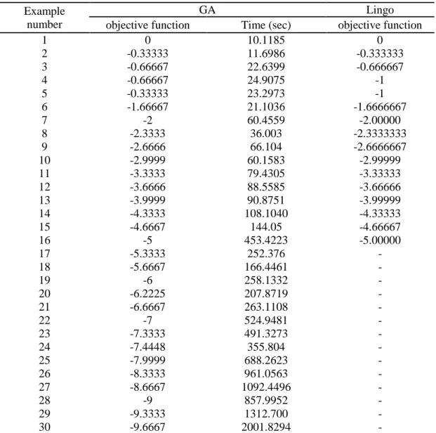
It should be noted that the proposed meta-heuristics were coded using MATLAB software, version 7.11.00584 on a notebook with 4 GB memory and Core i5 processor. Also, Lingo 8.0 was used in order to evaluate the model validity and quality of the generated solutions by GA algorithm. However, due to the complexity of the proposed problems, Lingo software can only be run in small problem instances. Thus, in this state, objective functions were merged using LP-metric. Table 4 represents the results of applying GA algorithm and Lingo software in the designed examples.

Table 4. Results of applying GA algorithm and Lingo software in the designed examples

Lingo GA

Example

number objective function Time (sec) objective function 0 10.1185 0 1 -0.333333 11.6986 -0.33333 2 -0.666667 22.6399 -0.66667 3 -1 24.9075 -0.66667 4 -1 23.2973 -0.33333 5 -1.6666667 21.1036 -1.66667 6 -2.00000 60.4559 -2 7 -2.3333333 36.003 -2.3333 8 -2.6666667 66.104 -2.6666 9 -2.99999 60.1583 -2.9999 10 -3.33333 79.4305 -3.3333 11 -3.66666 88.5585 -3.6666 12 -3.99999 90.8751 -3.9999 13 -4.33333 108.1040 -4.3333 14 -4.66667 144.05 -4.6667 15 -5.00000 453.4223 -5 16 -252.376 -5.3333 17 -166.4461 -5.6667 18 -258.1332 -6 19 -207.8719 -6.2225 20 -263.1108 -6.6667 21 -524.9481 -7 22 -491.3273 -7.3333 23 -355.804 -7.4448 24 -688.2623 -7.9999 25 -961.0563 -8.3333 26 -1092.4496 -8.6667 27 -857.9952 -9 28 -1312.700 -9.3333 29 -2001.8294 -9.6667 30

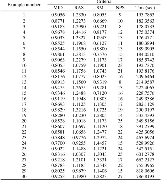
Data placed in Table 4 show that GA algorithm was accurately performed. Now, using MID, RAS, SM, NPS, and time criterion, the performance of NSGA-II algorithm was evaluated in 30 designed examples for the proposed combinational model and results are shown in Table 5.

Table 5. Results of applying NSGA-II algorithm and Lingo software in the designed examples Criteria Example number Time(sec) NPS SM RAS MID 193.7863 9 0.8055 1.2330 0.9056 1 182.3563 10 0.6669 1.2273 0.8771 2 178.0733 8 0.9221 1.2990 0.9183 3 175.0374 12 0.8177 1.4416 0.9678 4 176.4771 13 1.0943 1.2327 0.9033 5 180.3894 11 0.6127 1.1968 0.8525 6 189.0905 13 0.9800 1.1550 0.8544 7 184.0510 15 0.7576 1.3813 0.9861 8 185.5743 17 1.1173 1.2279 0.9063 9 192.7370 23 1.1901 1.0759 0.8055 10 193.8176 21 1.0743 1.1758 0.8546 11 209.6464 16 0.8023 1.0777 0.8176 12 214.9587 8 0.9319 1.1560 0.8913 13 222.4065 13 0.9281 1.2675 0.9475 14 228.7576 16 0.7120 1.2488 0.9346 15 249.3386 16 1.0803 1.1948 0.9119 16 282.1129 17 1.1305 1.1125 0.8693 17 290.0197 19 1.0725 1.3216 0.9829 18 333.4393 14 1.2805 1.0230 0.8280 19 349.5156 25 1.1173 1.1018 0.8528 20 391.2799 18 1.1120 1.0697 0.8607 21 425.3056 22 1.2477 1.0658 0.8581 22 463.6974 24 1.2972 0.9776 0.7848 23 528.9926 15 1.4457 0.9255 0.7700 24 542.5151 24 1.1221 1.1488 0.9022 25 601.2778 25 1.3043 1.0307 0.8316 26 662.2127 17 1.3331 1.2101 0.9218 27 755.3965 22 1.2548 1.1185 0.8783 28 818.0606 15 1.1406 0.9679 0.8025 29 786.8193 27 1.2823 1.1980 0.9253 30

Figures 1 and 2 demonstrate the performance of GA and NSGA-II in example 24 in order to better description of table results mentioned above.

Figure2. Performance of NSGA_II in example 2

5- Conclusion and suggestions for future work

Despite the past studies in covering literature, the absence of a comprehensive model to meet all practical requirements is absolutely undeniable. So it is necessary to define a new model through a specified framework of assumptions. In general, majority of covering models have been defined to cover a large volume of customer demands. In this paper, we have focused on emergency services in which responding to customers should be accelerated. Many customers (demand nodes) can’t tolerate waiting. This feature will reach to its summit in the scope of emergency services in which a slight delay can lead to serious problems. There is no time to loaf in such situations; accordingly, unavailability of servers should be assumed and solved. Even if it can be proved that the proposed covering model is comprehensively formulated, invalid and imprecise data will threaten its credibility. To overcome this problem, we addressed uncertainty in data by defining input and output values as intervals. Moreover, facilities should be located efficiently to stop disturbing the performance of other elements, to tackle this problem; we addressed efficiency by applying interval full-ranking model. All features mentioned above bring about a three-objective model which addresses availability, certainty and efficiency at the same time.

Different covering models include variant assumptions. That is why focusing on these assumptions can be a practical way for figuring out variant areas of future research. For instance, covering models can be called with different facilities, different covering radius, fuzzy and probabilistic parameters, and multi-objective covering models considering non-cost multi-objective functions. In addition to assumptions, focusing on solving methods can be considered as another practical area for future research. For instance, replacing GA with other solving algorithms like simulated annealing (SA) and Tabu search, the possibility of using hybrid systems for solving model, using stochastic programming solution techniques, and extending better heuristic methods can be effective.

References

Baron, B., Berman, O., Kim, S. and Krass, D. (2009). Ensuring feasibility in location problems with stochastic demands and congestions. IIE transactions, 41, 467-481.

Berman, O., Drenzer, Z., Krass, D. and Wesolowsky, G.O. (2009). The variable radius covering problem. European Journal of Operational Research, 196, 516-525.

Berman, O. and Wang, J. (2011). The mini-max regret gradual covering location problem on a network with incomplete information of demand weights. European Journal of Operational Research, 208, 233-238. Chou, S.Y., Chang, Y.H. and Shen, C.Y. (2008). A fuzzy simple additive weighting system under group decision making for facility location selection with objective/subjective attributes. European Journal of Operational Research, 189, 132-145.

Church, R.L. and Revelle, C. (1974). The maximal covering location problem. Papers of the Regional Science Association, 32, 101-118.

Daskin, M.S. (1995). Networks and discrete location: Models, algorithms and applications. NewYork, US: John Wiley and Sons.

Daskin, M.S. and Stern, E.H. (1981). A hierarchical objective set covering model for emergency medical service vehicle deployment. Transportation Science, 15, 137-152.

Erdemir, E.T., Batta, R., Spielman S., Rogerson, P.A., Blatt, A. and Flanigan, M. (2010). Joint ground and air emergency medical services coverage models: A greedy heuristic solution approach. European Journal of Operational Research, 207, 736-749.

Ghodratnama, A., Tavakkoli-Mogaddam, R. and Azaron, A. (2015). Robust and fuzzy goal programming optimization approaches for a novel multi-objective hub location-allocation problem: A supply chain overview. Applied Soft Computing, 37, 255-276.

Hakimi, S.L. (1965). Optimum distribution of switching centers in a communication network and some related graph theoretic problems. Operational Research, 13, 462-475.

Hogan, K. and Revelle, C. (1986). Concepts and applications of backup coverage. Management Science, 32, 1434-1444.

Hosseininezhad, J., Jabalameli, M.S. and Jalali Naini, GH. (2014). Fuzzy algorithm for continuous capacitated location allocation model with risk consideration. Applied Mathematical Modeling, 38, 983-1000.

Kolen, A. and Tamir, A. (1990). Covering problems, In: P.B. Mirchandani, R.L. Francies (Eds.), Conf. Discrete Location Theory, Wily, New York, 263-304.

Lannoni, A.P. and Morabito, R. (2007). A multiple dispatch and partial backup hypercube queuing model to analyze emergency medical systems on highways. Transportation Research, 43, 755-771.

Lee, J.M. and Lee, Y.H. (2010). Tabu based heuristics for the generalized hierarchical covering location problem. Computers and Industrial Engineering, 58, 638-645.

Martinez-Salazar, I., Molina, J., Ángel-Bello, F., Gómez, T. and Caballero, R. (2014). Solving a bi-objective Transportation Location Routing Problem by meta-heuristic algorithms. European Journal of Operational Research, 234, 25-36.

Moheb-alizade, H., Rasouli, S.M. and Tavakkoli-mogaddam, R. (2011). The use of multi-criteria data envelopment analysis for location-allocation problems in a fuzzy environment. Expert Systems with Applications, 38, 5687-5695.

Ni, Y., (2012). Minimum weight covering problems in stochastic environments. Information Sciences, 214, 91-104.

Owen, S.H. and Daskin, M.S. (1998). Strategic facility location: A review. European Journal of Operational Research, 111, 423-447.

Peijun, G. (2009). Fuzzy data envelopment analysis and its application to location problems. Information Sciences, 179, 820-829.

Pereira, M. and Coelho, L. (2015). A hybrid method for the probabilistic maximal covering location-allocation problem. Computers and Operations Research, 57, 51-59.

Pirkul, H. and Schilling, D. (1989). The capacitated maximal covering location problem with backup service. Annals of Operational Research, 18, 141-154.

Revelle, C. and Hogan, K. (1989). The maximum reliability location problem and a-reliable p-center problems. Annals of Operational Research, 18, 155-174.

Sohrabi Haghighat, M. and Khorram, E. (2005). The maximum and minimum number of efficient units in DEA with interval data. Applied Mathematics and Computation, 163, 919-930.

Thomas, P., Chan, Y., Lehmkuhl, L. and Nixon, W. (2002). Obnoxious-facility location and data envelopment analysis: A combined distance-based formulation. European Journal of Operational Research, 141, 495-514.

Toregas, C., Swain, R., Revelle C. and Berman L. (1971). The location of emergency service facilities. Operational Research, 19, 1363-1373.

Tsou, C.S. (2009). Evolutionary Pareto optimizers for continuous review stochastic inventory systems. European Journal of Operation Research, 195, 364-371.

Vidyarthi, N. and Jayaswal, S. (2014). Efficient solution of a class of location–allocation problems with stochastic demand and congestion. Computers and Operations Research, 48, 20-30.

Wen, M. and Kang, R. (2011). Some optimal models for facility location-allocation problem with random Fuzzy demands. Applied Soft Computing, 11, 1202-1207.

Zanjirani, R., Asgari, N., Heidari, N., Hosseininia, M. and Goh, M. (2012). Covering problems in facility location: A review. Computers and Industrial Engineering, 62, 368-407.

Zarandi, M.H., Davari, S. and Haddad Sisakht, A. (2013). The large-scale dynamic maximal covering location problem. Mathematical and Computer Modeling, 57, 710-719.