Identification and Removal of Low Energy Noise Events in the MAJORANA
DEMONSTRATOR Using Wavelet Transforms
Drew Smith∗
Department of Physics and Astronomy, University of North Carolina, Chapel Hill, NC
The MAJORANA DEMONSTRATOR is an array of enriched, high-purity Germanium (HPGe) p-type point contact (PPC) detectors constructed to demonstrate the necessary background rates for the detection of neutrinoless double-beta decay and establish the feasibility of a tonne-scale experiment. The PPC detectors have excellent electronic noise performance, providing the oppor-tunity to perform searches for various types of dark matter and other BSM physics that manifest at low energy. In this study we identify some sources of noise events in low-energy (<200 keV) regions and discuss their removal. These methods are based on the offline calculation of parameters that are sensitive to a signal's risetime. In particular, the relationship between two of these parameters (wpar and T/E) is considered in detail, and an attempt is made to place a cut on the data using
this 2-dimensional distribution.
I. INTRODUCTION
A. The MAJORANA DEMONSTRATOR and the
Motivation for Low Energy Data Cleaning
The MAJORANA DEMONSTRATOR is a 40-kg col-lection of high purity germanium (HPGe) detectors, of which about 30-kg is enriched to 87% in76Ge. Currently, there are two separate cryostats which each host about 20 kg of germanium. In each cryostat, the germanium is distributed as 7 strings, with each string holding up to 5 detectors each. The main goal of the MAJORANA DEMONSTRATOR is to demonstrate low enough back-ground rates and establish the feasibility of a tonne-scale experiment to detect neutrinoless double-beta de-cay. To accomplish this task, a background rate of 3 counts/tonne/year in the 4 keV region around the 76Ge endpoint energy is desired.
Fig. 1: A p-type point contact detector and its normalized weighting potential [8].
∗Electronic address: [email protected]
The P-type point contact (PPC) detectors used in the MAJORANA DEMONSTRATOR provide many advan-tages for achieving this goal. First, they have very even weighting potentials throughout the bulk of the detec-tors, which greatly increase around the point contact. This allows for easy distinction between single-site and multi-site events due to their different signal shapes. Sec-ond, due to the small size of the point contact (see Fig-ure 1), PPC detectors have very low capacitances (on the order of 1 pF), and allow for detection of sub-keV events. This feature of PPC detectors provides the MA-JORANA Collaboration with the opportunity to perform direct searches for weakly interacting dark matter by at-tempting to measure the nuclear recoil signals of dark matter collisions in the detectors.
A The MAJORANA DEMONSTRATOR and the Motivation for Low Energy Data CleaningI INTRODUCTION
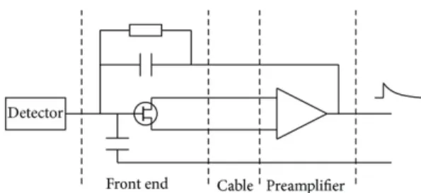
Fig. 2: A high level illustration of the detector electronics for the MAJORANA DEMONSTRATOR.
This figure was taken from [1].
B. Data Acquisition for the MAJORANA DEMONSTRATOR
The data acquisition process for the MAJORANA DEMONSTRATOR is handled by the Objectoriented Real-time Control and Acquisition (ORCA) system. ORCA provides a graphical representation of the experi-mental hardware and configurations in the MAJORANA DEMONSTRATOR, and allows for easy manipulation of the electronic configuration to best suit specific experi-ments. A more detailed description of the ORCA system can be found in [6].
The detector electronics configuration is illustrated in Figure 2. Each circuit features a Field Effect Transistor, as well as a pre-amplifier and several feedback compo-nents. Furthermore, the MAJORANA DEMONSTRA-TOR uses GRETINA (Gamma-Ray Energy Tracking In-beam Nuclear Array) digitizer cards which are a com-bination of digiziters and digital signal processors. The signal processors can accept up to 10 inputs from the de-tector pre-amplifiers, and digitize the data at a frequency of 100 MHz with 14 bit ADC precision [1]. Therefore, the digital signals that are measured are sampled at a rate of 1 sample per 10 ns. A more complete discussion of the electronics used in the MAJORANA DEMONSTRATOR can be found in [5].
C. Wavelet Transforms
Following [5], the approach taken in this project to identify and remove noise events involves the use of wavelet transforms. Wavelet theory is a relatively new branch of applied mathematics used to provide a mul-tiresolution analysis of a given signal. Similar to how windowed fourier transforms give insight into the fre-quency components of a signal while also providing some degree of time localization, wavelet transforms convert a signal of finite energy from the time domain into the 2-dimensional time-scale space, where different scales give information about different frequency components present in the signal. Because wavelet transforms are used so heavily in this study, a mathematical foundation for the theory behind them should be discussed.
First, we describe what a wavelet actually is. A func-tion, ψ L2 (where L2 represents the Hilbert space of square integrable functions), can be called an orthonmal wavelet if it can be used to define a complete, or-thonormal basis for the Hilbert space domain. This ba-sis is typically formed by dyadic dilations of the original wavelet function:
ψn,i(t) = 2 n
2ψ(2nt−i) (1)
for ∀n, i Z. In this case, n defines the scale of the wavelet. The larger n, the smaller the scale (i.e. ψ is shrunk), and the information contained in the transform concerns higher frequency components present in the sig-nal. Because the family of wavelets, ψn,i forms a com-plete basis for the domain of square integrable Hilbert space, any function in that domain can be written as linear combination of them. Mathematically,
f(t) = ∞
X
n,i=−∞
cn,iψn,i(t) (2)
for∀f(t) L2. This representation of the function,f(t), is called a wavelet series. The continuous wavelet trans-form can then be constructed using the following integral:
ˆ
f(a, b) = √1
a Z ∞
−∞
ψ∗ t−b
a
f(t)dt (3)
wherea= 2−n,b=k2−n, andf(t) is the original signal. In the Discrete Wavelet Transform (DWT), a signal is transformed at multiple levels into sets of approximation and detail coefficients. In [7], this process is described as a signal passing through a series of cascaded high and low pass filters. We defineGto be the impulse response of the low pass filter,H to be the impulse response of the high pass filter, andX to be the discretized signal. The first step in the DWT is to convolveX with the low pass filter to approximate the function:
cA[i] = ∞
X
k=−∞
X[k]G[i−k]
cD[i] = ∞
X
k=−∞
X[k]H[i−k]
(4)
C Wavelet Transforms II THE ”WAVELET PARAMETER”
Fig. 3: An illustration of the DWT. Here a discretized input signal,X[i], is passed through a series of cascaded
high-pass (H0) and low-pass (G0) filters. The output of the low-pass filters serve as an approximation of the input signal, and are then passed down to the next level
where they are fed through another layer of filters [5].
coefficients from the previous level through the next set of high and low pass filters. Next, the approximation coefficients, cA are fed through another set of high and low pass filters to generate another set of approximation and detail coefficients. An illustration of this process is provided in Figure 3. The high pass filter, H, used at each level of the transform is the mother wavelet chosen for the algorithm, and Gis the quadrature mirror filter ofH (i.e. H[z] =G[−z]).
The notation for wavelet transforms is not consistent among the scientific community, so for consistency, we define the levels of anm-th level wavelet transform by it-erating reversely at each stage of the transform, starting fromm−1. For example, in an 8-level DSWT, the n=7 level detail coefficients are the output of the first con-volution of the signal with the high pass filter (i.e. cD from Eq. 4), and represent the highest frequeny compo-nents present in the signal. Conversely, the n= 0 level detail coefficients are the output of the final high-pass fil-ter in the process and relay information about the lower frequency components in the signal.
In this study, a Haar wavelet is used as the mother wavelet for all transforms due to its close resemblance to a signal from a PPC detector. The Haar wavelet is essentially a square wave, or step function that ”steps” from 1 to -1. As a result, the detail coefficients of the nth level of an m-level DSWT represent the difference between the average of 2m−n adjacent samples and the previous 2m−n samples:
c(Di)(n) = 1 2m−n
2m−n
X
k=0
X[i−k]−
2m−n
X
k=0
X[i+k]
(5)
For this reason, the detail coefficients of the wavelet transform are essentially smooth derivatives of the sig-nal, with the smoothness being determined by the scale of the transform (the higherm is, the more smooth the
n= 0 detail coefficients will be). Figure 4 shows a signal from the MAJORANA DEMONSTRATOR as well as 8 levels of its detail coefficients after the DSWT algorithm was applied using a Haar wavelet.
Fig. 4: Plotted on top is a typical signal from the MAJORANA DEMONSTRATOR. The next 8 plots are
the detail coefficients resulting from an 8-level DSWT of the input signal using a Haar Wavelet. Note that the
bottom plot is the n= 0 level detail coefficients.
II. THE ”WAVELET PARAMETER”
A. Definition of wpar
With the knowledge of wavelet transforms, one can define a ”wavelet parameter”,wpar, using the detail co-efficients of a particular signal. In [3], this parameter is defined as
wpar =
max|c(Di)(n= 0)|2 E2
where c(Di)(n = 0) are the n = 0 order detail coeffi-cients (i.e. the lowest freuency detail coefficoeffi-cients in the wavelet transform), andE is the signal0s estimated en-ergy. The scale at which one chooses to definewpar de-pends on how many levels of the transform one wishes to apply. As more levels are applied, the detail coef-ficients of the n = 0 level will increase in scale (recall that n is iterated inversely to zero on each new level of the transform), and conversely, the detail coefficients re-lay information about lower frequency components of the signal. In [5], an 8-level wavelet transform was used to calculatewpar for data from MALBEK (Majorana Low-Background BEGe at KURF), a single 465 g Broad En-ergy Germanium (BEGe) detector installed at Kimball-ton Underground Research Facility (KURF). However,
A Definition ofwpar II THE ”WAVELET PARAMETER”
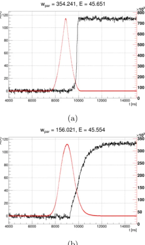
To demonstrate the effectiveness of wpar in identify-ing slow pulses, two signals of similar energies (E ≈45 keV) are shown in Figure 5 along with their n = 0 or-der detail coefficients's power spectrum after an 8-level wavelet transform. From these plots we see that good nuclear physics events (like the one in Fig. 5(a)) have much higher values of wpar than slow pulses of similar energies. This is because the rounded edge on the peak of the slow pulse signal causes the detail coefficients to have lower amplitudes than for signals with quick rise times and sharp edges.
(a)
(b)
Fig. 5: (a) A 45.65 keV signal (in black) plotted along with the power spectrum for then= 0 order detail coefficients (in red). (b) The same for a ”slow” event.
B. wpar Distributions
For an ideal signal (i.e. a square wave), the maximum value of the detail coefficients is directly proportional to the energy of the signal. Hence, one would expect the
wpar distribution for good events to be relatively con-stant as a function of energy. This is confirmed in Fig-ure 6, as the largest concentration of events falls on a straight line that is constant with energy. The width of this line increases as energy decreases, due to the increas-ing effect of noise on the signals. Because signals of all energies have relatively similar noise amplitudes mixed in with them, the signal to noise ratio decreases linearly
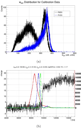
Fig. 6: 2-Dwpar-Energy distribution for a single detector. This data is taken from a set of228Th
Calibration runs.
Fig. 7: 1-Dwpar distributions at different energy ranges for the same detector and data as Figure 3. Note that the ”trapENFCal” mentioned in the legend is an offline
energy estimator, and has units of keV.
B wpar Distributions II THE ”WAVELET PARAMETER”
As expected, wpar is very detector-dependent. The
wparvalue of the good event peak in the detector-specific distributions can vary from detector to detector by as much as 30%. Additionally, the distribution of events outside the ”good event peak” in thewpar distributions, is often dramatically different for different detectors. An example is shown in Figure 8(a), in which the 1-D wpar distributions for event energies between 5 and 10 keV are plotted for two separate detectors. The obviouse dis-tinction between these two detectors'swpardistributions is the ”hump” present in the distribution for P6D3 (the black histogram). After going through some of the events that fell in that ”hump” region, it was found that these are mostly slow pulses. That said, however, there were many events in that region similar to the one shown in Figure 8(b). This is a very strange looking signal due to the fact that typically when an event occurs, after the detector collects all the charge deposited from the event, the charge axis begins to decrease slowly. However, in this event a certain amount of charge is collected very quickly, but then the charge continues to rise slowly -almost as if another small energy event occurred imme-diately afterwards.
Unfortunately it is difficult to pinpoint the specific rea-son why two detectors'swpardistributions appear so dif-ferent, as it could depend on a number of reasons. First, the dead-layer thickness of the PPC detectors is a large factor that determines the distribution of slow events. Logically, it is easy to see why thicker dead-layers lead to more surface events, but I have no way of directly measur-ing these thicknesses. Second, the location of a detector within the cryostat has an effect on the wpar distribu-tions. Detectors that have more neighboring detectors are more prone to events that scatter from a different detector. Often, these scattered events occur within the dead-layer of the detector, thus leading to a larger num-ber of slow pulses. Finally, the electronics are not entirely uniform from detector to detector. This creates small differences in the signals measured, which appear in the
wpar distributions. This effect likely does not lead to obvious changes in the shapes of the wpar distributions, but it does affect the location of the ”good event” peak in the distributions (for example, the black distribution in Fig. 8(a) has a peak atwpar≈330, while the blue dis-tribution has a peak at wpar ≈350. Because of this, it is necessary to perform detector-specific analyses ofwpar distributions, and as will be apparent later, it is neces-sary to create detector-specific cuts when attempting to usewpar to remove noise events.
C. wpar Optimization
There are only two choices one has to make when defin-ingwpar. The first is which wavelet to use as the mother wavelet (i.e. theψ(t) in eq. 3). As previously discussed, a
(a)
(b)
Fig. 8: (a) 1-Dwpar distributions for event energies between 5-10 keV two different detectors. (b) An example waveform in the ”hump” region in thewpar
distribution for P6D3. Also plotted on top of this waveform are then= 0 level detail coefficients of the signal after a wavelet transform with 8 levels (in red), 7
levels (in blue), and 6 levels (in green).
Haar wavelet was decided upon do its close resemblance to a PPC detector signal, and thus its ability to pick out important features along the rising edge of the sig-nals. The only other choose to make when definingwpar is how many levels of the wavelet transform one should apply. In [5], a similar study was done on data from MALBEK, where a wavelet parameter was defined using an 8-level wavelet transform. Therefore, this an 8-level transform is a good starting point for this study. How-ever, because detector electronics heavily affectwpar dis-tributions, it is necessary to see which level of a wavelet transform producewparvalues that are best suited to the task of identifying and removing slow pulses. A desirable
C wpar Optimization III T/E AND JOINTwpar-T/E DISTRIBUTIONS
wpar to not have a strictly linear relationship with T/E, a parameter that will be introduced in the following sec-tion. This is because if it were directly proportional to T/E, then it would provide us with little new insights into identifying noise events).
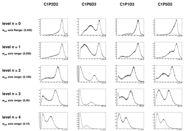
To accomplish this task ofwpar optimization, thewpar distributions for each detector were plotted when wpar was calculated using an 8, 7, 6, 5 and 4-level wavelet transform. The levels below 4 were also investigated, but there was almost no distinction between fast and slow events in those distributions. The resulting plots for four different detectors are shown in Figure 9.
Not many conclusions regarding the problem of wpar optimization can be made based solely on these plots because there is no way to know which events are slow pulses and which events are fast pulses. The first ap-proach taken to determine which level was most opti-mal was to simply browse the waveforms at different lo-cations in these distributions and see if there was any distinction between fast and slow pulses. Doing this re-vealed that many fast pulses were present in both peaks of the n=3 and n=4 levels. This is due to the fact that at those levels, the detail coefficients represent a less smooth derivative of the signal, and thus are much more sensi-tive to noise. In the n = 0, 1, and 2 levels, however, a quick browse through the largest peak revealed mostly fast pulses, so a more systematic approach needed to be taken to decide which of those levels was most optimal to use.
The next method employed was to place a cut on a small width of the main peak in the wpar distributions and see how the resulting spectra changed after the cut. As it turned out, though, each of these cuts produced ex-tremely similar spectra. So, the 8-level wavelet transform was chosen as the optimal level to use for calculations of
wpar mostly because the width of its fast pulse peak is the smallest.
III. T/E AND JOINT wpar-T/E DISTRIBUTIONS
A. Definition of T/E
Another parameter that is sensitive to the risetime of a signal is “T/E”, and is defined as the maximum output of a signal after passing through a triangle filter normalized by its energy. To perform the calculation, the GAT (Ger-manium Analysis Toolkit) library's GATTrapezoidalFil-ter class is used. GAT is a collection of software tools designed for the analysis of germanium detectors, and is used by the Majorana Collaboration [4]. One particu-larly useful tool in the GAT library is the trapezoidal fil-ter, which allows one to digitally convolve an input signal with a customized trapezoidal filter. The triangle filter used to calculate the “T” in “T/E” is constructed as a trapezoidal filter with 100 ns rise time, and 10 ns flat time (the signals in the MAJORANA DEMONSTRATOR are
sampled every 10 ns, so even though this is technically a trapezoidal filter, it essentially acts as a triangle filter due to its extremely small flat time). The output of that transform is then divided by the energy, as calculated with a trapezoidal filter with a rise time of 4 µs, a flat time of 2.5µs, and a non-linearity correction at a fixed time pickoff.
Likewpar, the value of T/E for good events is ideally a constant as a function of energy. This is confirmed by Figure 10(a), in which T/E is plotted against energy for a single detector using about 1 hour of228Th calibration data. One particularly useful feature of the T/E param-eter is that at low energies, it follows a bimodal distribu-tion. Figure 10(b) shows the 1-D T/E distribution for a single detector using only events between 5 and 10 keV. A quick glance through the events in the two peaks of Figure 10(b) reveals that the smaller-valued T/E peak is predominantly home to slow events, whereas the higher-valued T/E peak represents the good events.
B. Motivation for a Jointwpar-T/E Cut
Although both wpar and T/E can be seen as smooth derivatives of the signals, neither parameter deals with noise perfectly well. Consequently, both the T/E and
wparcalculations occasionally fail to identify slow events. As an example, the signal shown in Figure 11(a) was found to pass a cut placed on the ”good event peak” of the T/E distribution in Figure 11(b). This signal is very obviously a slow pulse, but a simple T/E cut would fail to remove it from the data. If a jointwpar and T/E cut were placed on the data, however, this particular event would in fact be removed due to its very lowwpar value. Cases like this provide the reasoning why a T/E cut by itself would not be an optimal method to identify and remove slow pulses.
On the other hand, there are a number of interesting signals that were found to fail a lone T/E cut, but pass a lone wpar cut. A typical example of this is displayed in Figure 11(b). Although it is more subtle, this signal is not a good event, as it has a very long risetime and a curved edge leading to its peak. As a result, its calculated value of T/E is fairly low. However, its calculated value ofwpar is actually fairly high. Based solely onwpar, this signal looks like a good physics event. The reason for
B Motivation for a Jointwpar-T/E Cut III T/E AND JOINTwpar-T/E DISTRIBUTIONS
Fig. 9: Thewpar distributions for 4 different detectors using different levels of the wavelet transform to calculate
wpar. These distributions were made using events with energies between 5 and 10 keV. Note that level n = 0 is the result of an 8-level wavelet transform, n = 1 is a 7-level transform, and so on.
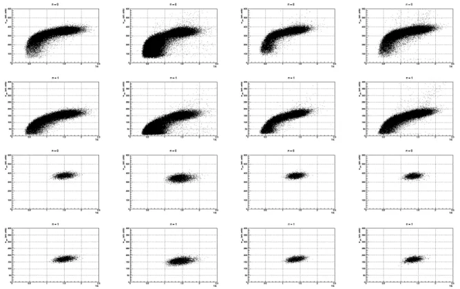
C. Jointwpar-T/E Distributions
The simplest way to study the relationship between
wpar and T/E is simply to plot the 2-dimensional dis-tributions of the two events for different energy ranges. Shown in the top two rows of Figure 12 are the wpar -T/E joint distributions for events between 5 and 10 keV for four different detectors. The first row was made by calculatingwpar using an 8-level wavelet transform, and the second row used a 7-level transform. Apparently, the relationship betweenwpar and T/E becomes more linear as the scale of the wavelet transform decreases. Although it is not shown here, the most linear relationship is ob-tained when using a 5-level wavelet transform to calcu-late wpar. This is not surprising, because as explained in section 1B, the n= 0 order detail coefficients for an m-level transform using a Haar wavelet are calculations of the average of 2m samples subtracted from the aver-age of the previous 2msamples. Because signals from the MAJORANA DEMONSTRATOR are sampled every 10 ns, whenwpar is calculated from a 5-level transform, the calculation time is about 320 ns, which is close to the 210 ns integration time from the triangle filter used to calculate T/E.
The bottom two rows of Figure 12 represent data from external pulsers. These data sets were recorded in the absence of a calibration source and the majority of the events are fast rising pulsers that were generated using a wavefunction generator and ran through the detectors's electronics. Hence, we can take the external pulser data to be an accurate depiction of the 2-D,wpar-T/E distri-bution for good events.
IV wpar-T/E CUT AND ESTIMATION OF EFFICIENCY
(a)
(b)
Fig. 10: (a) T/E vs. Energy calibration data distribution for a single detector. (b) The 1-D T/E Distribution for a single detector using only events with
energies between 5 and 10 keV.
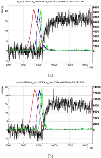
These plots of wpar vs. T/E for each detector also revealed some interesting types of events present in the data that would not have been uncovered otherwise. For example, in Fig 13(b), there is a number of events that show a strong correlation betweenwpar and T/E. It was later determined that these events only appeared in a small set of calibration runs, and thus are likely not good physics events (Unfortunately, I did not have the time to carefully determine the source of these events, but that should be an easy task for future investigation).
IV. wpar-T/E CUT AND ESTIMATION OF EFFICIENCY
Anytime a cut is placed on the data, a number of good events as well as bad are removed. The goal in generat-ing appropriate cuts is to remove as many bad events as possible, while keeping a high percentage of good events.
(a)
(b)
Fig. 11: (a) An example waveform highlighting the occasional negligence of a T/E cut to remove slow pulses. (b) An example waveform highlighting the inability ofwpar to deal with certain characteristics of signals. Also plotted on both waveforms are the power spectra of then= 0 order detail coefficients after an 8-level wavelet transform (in red), a 7-level transform
(in blue), and a 6-level transform (in green).
IV wpar-T/E CUT AND ESTIMATION OF EFFICIENCY
Fig. 12: wpar vs. T/E plots for calibration data, as well as external pulser data. The top row represents the distributions for four different detectors from calibration data when definingwpar using an 8-level wavelet transform. The second row is the same data, but uses a 7-level transform instead. Similarly the bottom two rows are the 8-level and 7-levelwpar vs. T/E distributions for the same detectors, but using only external pulser data. Note that every
plot in a given column is constructed using data from the same detector.
for the data. The solution was to take events at higher energies where the slow pulse and noise population was extremely small (almost non-existent), and scale them down to model events at lower energies.
Originally, the largest peak in the 228Th calibration spectrum was intended to be used for this task (the 2614 keV gamma ray peak). However, most of the events within this peak are actually multi-site events, as the gamma ray scatters around in the detector multiple times before being completely absorbed. Instead, the 1592 keV ”Double-Escape Peak” was used for scaling high energy events. Events that fall inside this peak are the result of the 2614 keV gamma ray entering a detector and creat-ing an electron-positron pair that annihilate and create two 511 keV annihilation photons. When both of these photons escape the detector, the total energy absorbed is equal to (2614 keV) - (2*511 keV) = 1592 keV. In [2] it is estimated that close to 80% of events in this peak are single site events.
The first major assumption made when scaling high energy events down to lower energies is that the ampli-tude of the noise present in a signal is independent of that signal's energy. This is a fairly reasonable assump-tion, as the noise in a signal is a result of the detector electronics, which is consistent for events of all energies. With that assumption in mind, the first step in
scal-ing these events was to sample the noise from the high energy events. If we define X to represent the original signal, with Xi being the ADC readout sample, i, in a background-subtracted signal, then we can represent the scaled signal as follows:
Yi=αXi+σi
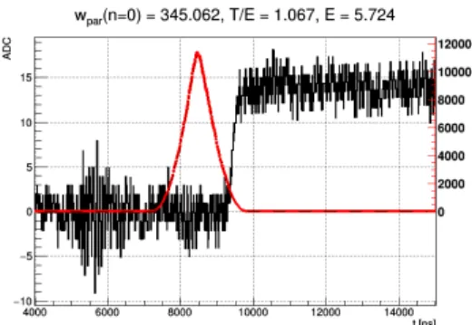
where Y is the scaled waveform, σi is an estimation of noise drawn randomly from the aforementioned noise his-togram, andα is equal to the desired scaled energy di-vided by the energy of the original signal. Finally, be-cause these waveforms are digital signals,Yiwas rounded to the nearest integer. An example of a scaled waveform can be seen in Figure 14. The wpar-T/E distributions that resulted from these scaled waveforms are very sim-ilar to the external pulser data from Figure 12, and are displayed for 4 different detectors in Figure 16.
The idea here was to use scaled events in the range from 1-10 keV to create a cut, because events at low energies have the widest distributions. After a suitable cut was determined, the percentage of scaled events that passed the cut would serve as an estimate for the good event acceptance efficiency. Because the shapes of the
IV wpar-T/E CUT AND ESTIMATION OF EFFICIENCY
(a)
(b)
Fig. 13: (a) Thewpar-T/E distribution of events between 1 and 3 keV. (b) The same distribution for the
same detector and calibration data, but for events between 15 and 25 keV.
Fig. 14: A 5.5 keV waveform scaled down from the 1592 keV double escape peak.
scaled events distributions. This was carried out sys-tematically by first projecting the 2-D histograms into a profile histogram along the T/E axis, and fitting the re-sult to a straight line. The rere-sulting slope of the fit was used as the slope for the top and bottom edges of the quadrilateral cut (because this was only intended to be a
starting point, the left and right edges of the quadrilat-eral cuts were created as vertical lines parallel with the
wparaxis). An illustration of this initial quadrilateral cut is seen plotted on top of the distributions in Figure 16.
Fig. 15: A 5.7 keV signal along with itsn= 0 order detail coefficients power spectrum plotted in red.
After suitable cuts had been determined for each de-tector (again, I’d like to reiterate that wpar and T/E are very detector-dependent parameters, and thus re-quire detector-specific analyses), a summed calibration spectrum was constructed both before and after apply-ing the cuts. However, initially the resultapply-ing spectrum contained a much lower number of events at energies be-low 10 keV than expected. After some diagnostics, the source of this issue was revealed to be that thewpar dis-tributions of the scaled events for some detectors did not align with thewpar distributions of actual events of simi-lar energies. Specifically, there were 5 detectors that very obviously did not align with the calibration data, and two others that were very questionable. As an example, Fig-ure 17 shows the wpar distributions for 2 detectors for both the scaled events, and actual calibration data (the energy range of these events is 1-10 keV). Notice that in C1P1D2, the scaledwpar distributions matched the ac-tual calibration data's fast peak quite nicely, whereas in C1P1D3, this is not the case. The reason for the differ-ence in thewpar distributions is not entirely clear at this moment, but it likely has something to do with the way noise is approxmated on the scaled signals. For example, Figure 15 shows a typical signal of about 5.7 keV from the calibration data. The obvious difference between this signal and the scaled waveform from Figure 14, is that in this one, the noise is not entirely uniform, but instead has bursts of increased amplitude. However, because the noise that is placed on the scaled waveforms is sampled from a histogram, there is no way to account for the tem-poral variance of the noise.
vulner-V CONCLUSION AND FUTURE IMPROVEMENTS
ability to noise at low energies.
There was no attempt to measure the slow pulse re-jection efficiency in this project, as detailed simulations are required to fully understand the distribution of slow pulses in a given detector. With some knowdledge of the percentage of slow events in each detector, an estimate of the rejection efficiency can be made just by consider-ing the total number of events before and after a cut, as well as the fast pulse acceptance efficiency. However, at this point, there is no clear indication as to the number of slow pulses present in the data, and the simulations required to answer that question are outside the scope of this project.
V. CONCLUSION AND FUTURE
IMPROVEMENTS
Although the relationship between wpar and T/E is still not fully understood, it is clear that both parameters can be effective tools in identifying slow pulses and other noise events. Unfortunately, a clear limitation of both parameters is their inability to effectively distinguish fast pulses from slow pulses at energies below about 3 keV. One approach to address this issue is to find a clever way to denoise waveforms at low energies before calculat-ing parameters such aswpar and T/E. Both parameters can be thought of as the output of a signal after pass-ing through some kind of filter, so we initially believed that the noise present in signals would not be too large of a factor. However, as discussed towards the end of
the previous section, the noise in these signals is not per-fectly gaussian noise, but instead has a slight temporal variability. If more efforts went in to understanding the noise of these waveforms, perhapswpar and T/E would become greatly more effective at lower energies.
Another improvement that can be made to the wpar -T/E cut is to create cuts that are dependent upon en-ergy. We previously saw that while the fast pulse peak in the wpar distributions remains relatively constant as a function of energy, the width of that peak increases as energy decreases (T/E is the same). Therefore, in order to obtain a larger fast pulse acceptance efficiency at low energies, one can place a more lenient cut on the data at those energies. Careful consideration should be made in this scenario to avoid an artificial detection of a WIMP signal, as this type of cut can lead to higher counts at lower energies, and can resemble a typical dark matter signature.
Acknowledgments
The work done in this project was completed over two semesters as part of a senior honors thesis independent study. Dr. Reyco Henning served as the faculty adviser for the project, and much is to be credited to his insights and expertise. Additionally, a number of nuclear physics graduate students at UNC-CH helped support this re-search in some form. In particular, huge thanks go to Kris Vorren for his development of the T/E parameter, as well as Ben Shanks for his initial guidance in working with the raw waveforms.
1
Abgrall, N., Aguayo, E. Avignone, F., et al., The MAJORANA DEMONSTRATOR Neutrinoless Double-Beta Decay Experiment, Advances in High Energy Physics, vol. 2014, Article ID 365432, 18 pages, 2014. doi:10.1155/2014/365432
2 Bakalyarov A.M., Balysh A.Ya., Belyaev S.T., Lebedev
V.I., Zhukov S.V. ”Identification of single events in the HPGe detector: Comparison of various methods based on the analysis of simulated pulse shapes.”
3 Finnerty, P.S.A Direct Dark Matter Search with the
Low-Background Broad Energy Germanium Detector.PhD The-sis, University of North Carolina at Chapel Hill, 2013.
4 Germanium Analysis Toolkit.
https://github.com/mppmu/GAT
5
Giovanetti, Graham K.P-Type Ppint Contact Germanium Detectors and Their Applications in Rare Event Searches.
PhD Thesis, University of North Carolina at Chapel Hill, 2015.
6 Howe, M., Cox, G., Harvey, P., McGirt, F., Rielage, K.,
Wilkerson, J., Wouters, J., IEEE Trans. Nucl. Sci., vol. 51, pp. 878883, 2004.
7 Mallat, S. G. A theory for multiresolution signal
decom-position: the wavelet representation, IEEE Trans. Pattern Anal. Mach. Intell. 11 no. 7, (1989) 674693.
8 Martin, R. ”PPC Ge Detectors for Dark Matter,
Neutrino-less Double Beta Decay and CNS Meausurements.” Power-point Presentation from the Coherent Neutrino Scattering Experiment Workshop, Texas A& M. 12 Nov,2015.
9 Schramm, Steven. ”Introduction and Motivation for Dark
V CONCLUSION AND FUTURE IMPROVEMENTS
Fig. 16: Thewpar vs. T/E distributions for events from the 1592 keV double escape peak that were scaled down to low energies. Each plot is for a different detector, and the scaled waveforms included in these plots were for events
between 1 and 10 keV.
(a) (b)
V CONCLUSION AND FUTURE IMPROVEMENTS
![Fig. 1: A p-type point contact detector and its normalized weighting potential [8].](https://thumb-us.123doks.com/thumbv2/123dok_us/8335006.2212233/1.918.128.400.735.965/fig-type-point-contact-detector-normalized-weighting-potential.webp)
![Fig. 3: An illustration of the DWT. Here a discretized input signal, X[i], is passed through a series of cascaded](https://thumb-us.123doks.com/thumbv2/123dok_us/8335006.2212233/3.918.114.396.83.174/fig-illustration-discretized-input-signal-passed-series-cascaded.webp)