Sharif University of Technology
Scientia IranicaTransactions A: Civil Engineering http://scientiairanica.sharif.edu
Standard equations for predicting the discharge
coecient of a modied high-performance side weir
A.H. Zaji
a;, H. Bonakdari
a, and Sh. Shamshirband
ba. Department of Civil Engineering, Razi University, Kermanshah, Iran.
b. Department of Computer System, Faculty of Computer Science and Information Technology, University of Malaya, 50603 Kuala Lumpur, Malaysia.
Received 4 March 2016; received in revised form 15 December 2016; accepted 31 July 2017
KEYWORDS Discharge coecient; Modied triangular side weir;
Nonlinear regression; Particle swarm optimization; Standard equation.
Abstract. Side weirs are hydraulic structures that are used as discharge adjustments to divert the surplus water owing from the main channel. Predicting the discharge coecient is one of the most important parameters in the side weir design process. In practical situations, it is preferred to predict the discharge coecient with simple equations. The goal of this study is to develop accurate standard equations for use in predicting the discharge coecient of a high-performance, modied triangular side weir. The Particle Swarm Optimization (PSO) algorithm was used to optimize the parameters of the equations. Four dierent forms of the equations and two non-dimensional input combinations were used to develop the most appropriate model. The results obtained by our simple standard equations optimized by the PSO algorithm were compared with those of complex nonlinear regression equations, and our equations were more accurate in modeling the discharge coecient. Our method reduced the error in the results by as much as 43% compared to the regression methods, and its simplicity makes it useful in solving practical problems. © 2018 Sharif University of Technology. All rights reserved.
1. Introduction
In some rivers, water and wastewater, irrigation, and drainage channel zones, the ow rate may exceed the tolerance capacity of a river or channel. In such a case, discharge control structures, such as side weirs, can be used to control the ow and prevent overows. Side weirs are also used to keep oods away from dam reservoirs and the diversion of ow for the sake of protection. The study of side weirs dates back to the early 20th century when De Marchi [1] laid the groundwork for other studies with his mathematical
*. Corresponding author.
E-mail addresses: [email protected] (A.H. Zaji); [email protected] (H. Bonakdari);
[email protected] (Sh. Shamshirband) doi: 10.24200/sci.2017.4198
model of side weirs. The equations he developed to describe side weirs were based on the assumption that the specic energy was the same before and after the weirs.
In this paper, a model with a decreasing discharge equation is presented for a rectangular channel with a horizontal bed and a spatially-varied ow. The equation is:
dy dx =
Q gb2y3
dQ dx
1 Q2
gb2y2
= Qy
dQ dx
gb2y3 Q2; (1)
where dy=dx is the depth change along the channel, Q is the discharge of the ow, y is the depth of the ow, b is the width of the main channel, dQ=dx is the discharge change along the channel, and g is the acceleration of gravity. The discharge per unit length over the side weir equals:
dQ dx =
2 3CM
p
2g(y w)1=5; (2)
in which CM is the discharge coecient, also known
as the De Marchi coecient. By assuming that the specic energy is constant, the discharge in the channel would be:
Q = byp2g(E y): (3)
By inserting Eqs. (2) and (3) into Eq. (1), we obtain: dy dx = 4 3 CM b p
(E y)(y w)
3y 2E : (4)
Integrating the above equations and assuming CM
independent of x direction, we will have Eq. (5): x = 2C3b
M(y; E; w) + c; (5)
where is obtained from Eq. (6). Therefore, CM
obtained in the laboratory is calculated by substituting through Eq. (5) as follows:
(y; E; w)=2E 3wE w s
E y
y w 3 sin 1 r
E y E w: (6) Moreover, the length of the side weir is obtained from Eq. (7):
L = x2 x1=32Cb
M(2 1); (7)
in which 1 and 2 are obtained from Eq. (6) for
upstream and downstream of the weirs, respectively. Assuming that Q1and Q2are the upstream and
down-stream discharges, the amount of side weir discharge is obtained from Eq. (3).
Following De Marchi [1], many researchers have tried to calculate the side weir coecients (CM), and
most of them have considered CM as a function of the
upstream Froude number (Fr1) [2-6].
A signicant number of researches have been conducted to increase the eciency of the side weir by changing its geometrical situation, i.e. changing its rectangular crest to triangular, circular, or elliptical, causing an increase in both the length of the weir and the discharge coecient. Borghei and Parvaneh [7] designed a modied triangular side weir whose dis-charge coecient that was 2.33 times higher than a conventional side weir's in a rectangular channel. The authors used 200 test measurements and, nally, using the nonlinear regression method, determined an equation for the modied triangular side weir discharge coecient, i.e. Eq. (8):
CM =
0:18
Fr1
sin 0
0:71
0:15(Fr1)0:44+
w Y1 0:7
2:37 + 2:58
w sin 0
Y1
0:36 :
(8)
Soft computing methods are used as a new tool for calculating the side weir coecient, and many re-searchers have considered their application in predict-ing scour depth [8-13], determinpredict-ing ow characteristics in dierent open channels [14,15], modeling rainfall and predicting stream ow [16-22], modeling coastal algal blooms [23], evapotranspiration [24,25], combined open channel ow [26,27], sediment transport [28,29], predicting ground water levels [30], and forecasting the demand for water [31-33]. In estimating the side weir coecient, Bilhan et al. [34] studied dierent Articial Neural Network (ANN) methods, and found that they have much higher accuracy than multiple nonlinear and linear regression models do. Using Radial Basis Neural Network (RBNN), Regression Neural Network (RNN), and Genetic Expression Programming (GEP), Kisi et al. [35] predicted the triangular side weir discharge coecient. The results were compared with 2500 laboratory measurements, and it was found that ANN and GEP gave better results than regression methods. To determine side weir discharge coecients, Emin Emiroglu et al. [36] used an adaptive neuro-fuzzy technique (ANFIS), the results of which indicated the high accuracy of the ANFIS method for modeling the side weir discharge coecient. Some other studies have been published on modeling the triangular labyrinth side weir discharge using soft computing, all of which were proved better than the regression methods [37-42]. The objective of this study is to provide a prac-tical, simple equation for calculating the discharge coecient for a modied, high-performance triangu-lar side weir. The Particle Swarm Optimization (PSO) algorithm was used to optimize each of the equations considered. Four dierent equation forms were developed using the input parameters of Fr1
(upstream Froude number), w=L (weir height/weir length), Fr1=sine(0) (upstream Froude number/sine
(weir included angle/2)), w=Y1 (weir height/upstream
ow depth), and w sine(0)=Y
1 (weir height sine
(weir included angle/2)/upstream ow depth). Con-sidering dimension L (length) for w, L, and Y1, it is
obvious that all of the used input parameters are non-dimensional. Finally, the accuracy of each equation was examined and compared.
2. Experimental setup
In this study, the laboratory model of Borghei and Parvaneh [7] was used, including a rectangular ume that was 11 m long and 0.4 m wide. The glass walls of the channel were 0.66 m high. The outlet discharges from the main and tributary channels (Q2 and Qw)
were measured by standard V notches. The accura-cies of the water head and discharge measurements were 1 mm and 0:0001 m3/s, respectively. The
Table 1. Interval variations in experimental tests of Borghei and Parvaneh [7].
() L (m) w (mm) w=Y
1 Q1 (m3/s) Fr1 Number of runs
30 0.3 50, 75, 100, 150 0.46-0.83 0.019-0.030 0.19-0.96 40 0.4 50, 75, 100, 150
45
0.3 50, 75, 100, 150
0.46-0.83 0.019-0.030 0.19-0.96 55 0.4 50, 75, 100, 150
0.6 50, 100, 150
60
0.3 50, 75, 100, 150
0.46-0.83 0.019-0.030 0.19-0.96 50 0.4 50, 100, 150
0.6 50, 100, 150
70
0.3 50, 75, 100, 150
0.46-0.83 0.019-0.030 0.19-0.96 55 0.4 50, 75, 100, 150
0.6 50, 100, 150
Figure 1. Plan view of modied triangular side weir and the parameters used.
conditions, opening lengths (L), weir heights (w), weir oblique angles (0), and input discharges (Q
1). All of
the tests were conducted under certain conditions in which the upstream Froude number (Fr1) was at the
interval of 0.19-0.96. Table 1 provides the parameters whose variation intervals are observed in the laboratory tests. Figure 1 shows the schema of the modied triangular side weir and the parameters used.
3. Methods and materials
In this study, the Particle Swarm Optimization (PSO) method was used to determine an accurate equation to predict the discharge coecient. The design of this method was inspired by ocks of birds or schools of sh, because when they stay together, the likelihood of being caught reduces. This is called swarm intelligence. When sh make up a school, they follow only a few simple, yet systematic, rules; however, their behavior appears very complicated. In addition to the PSO algorithm, Ant Colony Optimization (ACO), Bees Algorithm (BA), and Articial Fish Swarm (AFS) are all considered swarm intelligence methods.
3.1. Particle Swarm Optimization (PSO) Kennedy and Eberhart [43] introduced the PSO. Initially, the authors intended to create a sort of social-based computational intelligence, independent of individual capabilities, i.e. individuals with normal intelligence quotients could make up a very intelligent community. Therefore, their study resulted in a reliable algorithm for optimization called Particle Swarm Op-timization (PSO), in which there are some particles in space, and each particle has a potential solution to the problem. Each particle follows a general and xed rule to move, called self-organization. Based on this rule, each particle remembers the present and past situations as well as the best-experienced situation through both the single particle and all of the particles. The new position of the particle is calculated from Eq. (9) as follows:
vi[t + 1] =wvi[t] + c
1r1(xpbest[t] xi[t])
+ c2r2(xgbest[t] xi[t]): (9)
In this equation, the rst term on the right side of the equation represents a particle's movement toward its
last movement; the second term indicates the velocity of a particle moving toward the best-known former position, and the third term shows the velocity of a particle moving toward the best previous position experienced by all particles. Herein, xpbest is the
best personal memory, and xgbest is the best collective
memory. The inertia coecient (w) is an arbitrary factor that has values less than 1; r1and r2are random
numbers with a uniform distribution, while c1 and c2
are the individual and collective learning coecients, respectively, ranging between 0-2 [43]. The three terms are the resultant vector of the amount and direction of and movement towards a new position. Thus, from Eq. (10), we will get a new position of the particle as follows:
xi[t + 1] = xi[t] + vi[t + 1]: (10)
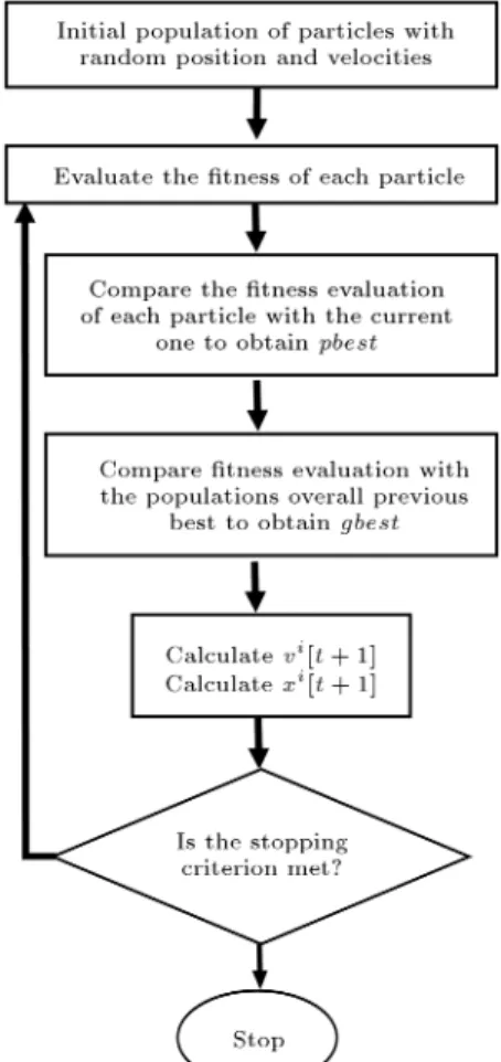
Figure 2 demonstrates the steps of the PSO algorithm. Initially, the primary population is formed; then, the tness function of each particle is determined. Subsequently, pbest and gbest are determined and,
then, memorized in the particle's memory. Eq. (9) is used to determine the particle's velocity, namely the direction and amount of the movement of the particle; subsequently, the velocity is added to the
Figure 2. Particle swarm optimization ow chart.
present particle's position to determine the particle's new position. Finally, the stopping criteria of the algorithm are checked. If the criteria have been met, the algorithm stops the process; otherwise, the loop is repeated. In all models here, the Number of Function Evaluation (NFE) is considered as a criterion for stopping the iterations at NFE = 100,000.
If the inertia parameter (w) reaches its maximum (w = 1), the algorithm's exploration property goes up; however, if w is low, the algorithm's exploitation property increases. It is generally expected that the exploration property be high at the beginning, while it increase at the end; therefore, in the algorithm used here, the damping coecient (wdamp= 0:98) was used
[44,45]. At the end of each repetition, the inertia parameter (w) decreases gradually, and as the results get closer to the end of the solution, w decreases, leading to an increase in the exploitation of the model (Eq. (11)):
w = w wdamp: (11)
3.2. Objective function and model performance In this study which uses the PSO algorithm, some equations are given for modeling the discharge coef-cient of a modied triangular side weir. The primary goal of PSO is to reduce the error that results from the proposed equation application, compared to the laboratory model. Therefore, according to Eq. (12), we have the following:
ei= fi f^i; (12)
where fi and ^fi are the results of the laboratory
model and the proposed equation, respectively. The algorithm uses Mean Square Error (MSE) to determine the iteration error, as shown in Eq. (13). In addition, in order to investigate the models' performance, Root Mean Squared Error (RMSE), Mean Average Error (MAE), and Mean Absolute Percentage Error (MAPE) are used (Eqs. (14)-(16)):
MSE = 1nXn
i=1
e2
i; (13)
RMSE = v u u t 1
n
n
X
i=1
e2
i; (14)
MAE = 1n
n
X
i=1
jeij; (15)
MAPE = Pn
i=1jeij
Pn
i=1fi
100
n ; (16)
4. Results
To estimate CM, four non-dimensional parameters
(Var1 to Var4) are considered as inputs in each of
the following equations. These parameters are a combination of the upstream Froude number (Fr1), side
weir oblique angle (0), weir height (w), and upstream
depth (Y1). As Eqs. (17) and (18) show, there are
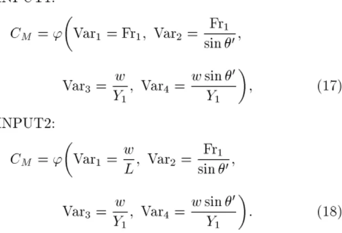
two possible input sets, i.e. INPUT1 and INPUT2, that can be considered for predicting the discharge coecient (CM). The dierence between the inputs
is that INPUT2 considers the four parameters (Y1, w,
0, Fr
1) as well as the length eect of the side weir
(L): INPUT1:
CM = '
Var1= Fr1; Var2= sin Fr10;
Var3=Yw
1; Var4=
w sin 0
Y1
; (17)
INPUT2: CM = '
Var1=wL; Var2= sin Fr10;
Var3=Yw
1; Var4=
w sin 0
Y1
: (18)
In order to study the eects of the considered input variables in Eqs. (17) and (18) on CM, the sensitivity
analysis of partial dierential equations is used [46,47]. In this method, the ratio of the change in CM (as the
output) to the change in the input variables considered in Eqs. (17) and (18) is examined. For the practical use of this method, the partial dierential equation can be approximated as a nite dierence [48] and output values calculated for the small changes in the input pa-rameters [49]. The sensitivities of Fr1;sin Fr10;Yw1;w sin Y1 ,
and w
L variables are {0.66, {0.22, 0:89, {3.28, and
1.27, respectively. Thus, w sin 0
Y1 and
w
L are the most
important input parameters where w sin 0
Y1 has a
neg-ative relation with CM and wL has a positive relation
with CM. In what follows, some standard equations are
optimized to estimate the discharge coecient (CM) by
the PSO algorithm; then, the error of each equation is calculated.
4.1. Optimized equation of Borghei and Parvaneh [7]
Eq. (19) represents the structure of Eq. (8) used by Borghei and Parvaneh [7]. Table 2 shows the coe-cients, i.e. a1 to a8, proposed in this study, estimated
through nonlinear regression. In Eq. (19), INPUT1 is considered as the input variable. MSE of the equation, related to the laboratory results, is equal to 0.0037 (Table 2). Figure 3(a) compares the calculated and laboratory results. The 45line is the exact solution to
the problem, and the closeness of the scatter to this line shows the accuracy of the model. Moreover, the t line equation (assuming that the equation is y = c1x + c2)
in Figure 3(a) shows the accuracy of the model and the deviation of the results from the exact line. Therefore, the closer c1 is to one and c2 is to zero, the greater
the accuracy of the model will be. In Figure 3(b), the laboratory results are compared with those of Eq. (8)
Table 2. Characteristics and statistical errors of Eq. (8).
INPUT1 Eq. (8)
a1 a2 a3 a4 a5 a6 a7 a8
{0.18 0.71 {0.15 0.44 0.70 {2.37 2.58 {0.36
MSE RMSE MAE MAPE
0.0037 0.016 0.0482 0.035
Figure 3. (a) Scatter plot of comparing the observed CM and the estimated CM by Eq. (8). (b) Comparison of the
to estimate CM. The horizontal axis represents the
number of datasets (200 tests), and the vertical axis shows the discharge coecient (CM). Figure 3(a)
shows that, in some parts, such as experiment numbers 20 to 40 and 100 to 120, there is a greater error in Eq. (8) than in the laboratory results. However, for intervals with a minor sudden change in the discharge coecient CM, such as experiment numbers 120 to 160,
the results are closer together:
CM = [a1(Var2)a2+ a3(Var1)a4+ (Var3)a5]
[a6+ a7(Var4)a8]: (19)
To nd an accurate and ecient equation for calcu-lating CM, coecients a1to a8were calculated by the
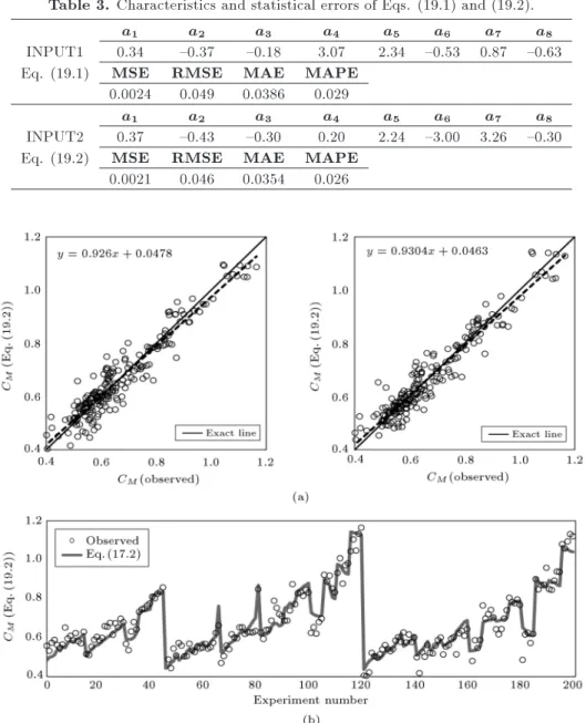
PSO algorithm, instead of nonlinear regression. Table 3 shows Eq. (19.1) calculated based on INPUT1 as the input variable. The table shows that MSE is equal to 0.0024, which is much lower than that of Eq. (8). In the next step, the input non-dimensional parameters were changed, and INPUT2 was used as an input variable for Eq. (19). Table 3 shows the related results obtained by Eq. (19.2). Since MSE decreased to 0.0021 while MSE of Eq. (19.1) was 0.0024, it is apparent that higher accuracy was attained using non-dimensional INPUT2. In Figure 4(a), the results from Eqs. (19.1) and (19.2) are given on the vertical axis; the laboratory test results are given on the horizontal axis. In both cases, the t line is very close to the exact line. Eq. (19.2), calculated based on INPUT2, has much higher eciency than Eq.
Table 3. Characteristics and statistical errors of Eqs. (19.1) and (19.2). INPUT1
Eq. (19.1)
a1 a2 a3 a4 a5 a6 a7 a8
0.34 {0.37 {0.18 3.07 2.34 {0.53 0.87 {0.63
MSE RMSE MAE MAPE
0.0024 0.049 0.0386 0.029 INPUT2
Eq. (19.2)
a1 a2 a3 a4 a5 a6 a7 a8
0.37 {0.43 {0.30 0.20 2.24 {3.00 3.26 {0.30
MSE RMSE MAE MAPE
0.0021 0.046 0.0354 0.026
Figure 4. (a) Scatter plot of comparing the observed CM and the estimated CM by Eqs. (19.1) and (19.2). (b)
(19.1). In Figure 4(b), the results of laboratory tests are compared with those obtained from Eq. (19.2). It is evident that the accuracy problems in Eq. (8) (Figure 3(b)) in test numbers 20 to 40 and 100 to 120 are almost solved; the results are agreeable.
4.2. Optimized 2nd-order equation
The main objective herein is to determine equations of high accuracy featuring simple standard forms. Therefore, the accuracy of the 2nd-order equations was investigated. Thus, CM equation resembles Eq. (20).
In this equation, a1 is the equation's constant value,
and a2 to a9 are the coecients that make the
2nd-order equation. In Eq. (20), Var1 to Var4 are used as
inputs from INPUT1 and INPUT2. Table 4 presents a1
to a9coecients as calculated from the PSO algorithm
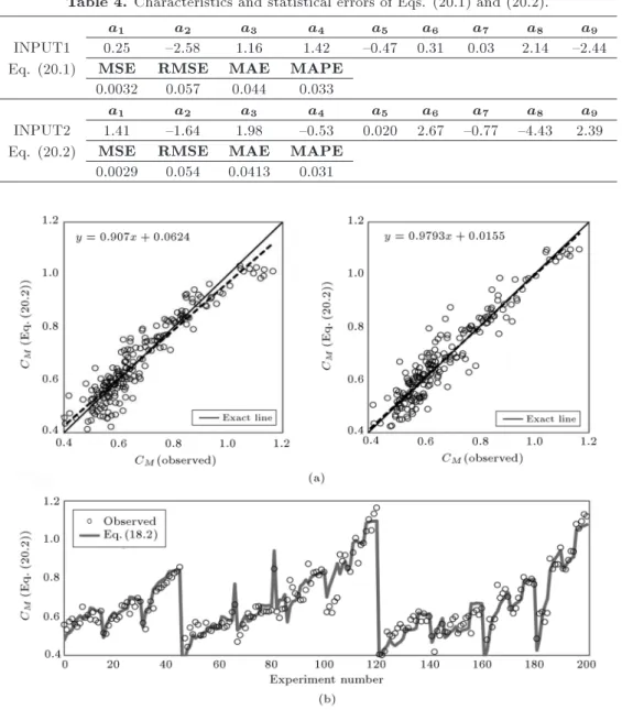
for Eqs. (20.1) and (20.2) with INPUT1 and INPUT2 as input variables, respectively. It is apparent that MSE in Eq. (20.2) using INPUT2 is less than that of Eq. (20.1) using INPUT1, indicating that INPUT2 combination gives more accurate results. Note that the very simple Eq. (20) gives much more accurate results than the complex Eq. (8) does. Higher MSEs in Eqs. (20.1) and (20.2) than those in Eqs. (19.1) and (19.2) may demonstrate that Eq. (19) has an optimized shape and is more ecient for modeling the discharge coecient of the modied triangular side weir. However, as stated above, the main advantage of Eq. (20) is its simplicity and its standard shape. In Figure 5(a), the estimated values of Eqs. (20.1) and (20.2) for INPUT1 and INPUT2 are plotted on the ordinate; the laboratory values are plotted on the
Table 4. Characteristics and statistical errors of Eqs. (20.1) and (20.2). INPUT1
Eq. (20.1)
a1 a2 a3 a4 a5 a6 a7 a8 a9
0.25 {2.58 1.16 1.42 {0.47 0.31 0.03 2.14 {2.44
MSE RMSE MAE MAPE
0.0032 0.057 0.044 0.033 INPUT2
Eq. (20.2)
a1 a2 a3 a4 a5 a6 a7 a8 a9
1.41 {1.64 1.98 {0.53 0.020 2.67 {0.77 {4.43 2.39
MSE RMSE MAE MAPE
0.0029 0.054 0.0413 0.031
Figure 5. (a) Scatter plot of comparing the observed CM and the estimated CM by Eqs. (20.1) and (20.2). (b)
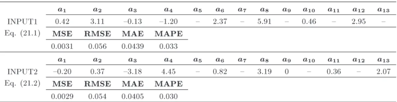
Table 5. Characteristics and statistical errors of Eqs. (21.1) and (21.2). INPUT1
Eq. (21.1)
a1 a2 a3 a4 a5 a6 a7 a8 a9 a10 a11 a12 a13
0.42 3.11 {0.13 {1.20 { 2.37 { 5.91 { 0.46 { 2.95 {
MSE RMSE MAE MAPE
0.0031 0.056 0.0439 0.033 INPUT2
Eq. (21.2)
a1 a2 a3 a4 a5 a6 a7 a8 a9 a10 a11 a12 a13
{0.20 0.37 {3.18 4.45 { 0.82 { 3.19 0 { 0.36 { 2.07
MSE RMSE MAE MAPE
0.0029 0.054 0.0405 0.030
abscissa. Note the excessive closeness of the t and exact lines of this equation to the extent that they overlap in Eq. (20.2). The closeness between these two lines means that errors in the data are scattered equally around the exact line. It could be inferred that this symmetry is due to the greater symmetry of Eq. (20) as compared to Eq. (19). Notice that this symmetry bears no relation to the accuracy of the model; for example, in Eq. (19.2), MSE (0.0021) is less than MSE of Eq. (20.2) (0.0029); however, in Eq. (20.2), c1 and c2 coecients are closer to 1 and
0, respectively, making the error results completely symmetrical. In Figure 5(b), the suggested results derived from Eq. (20.2) are presented with bold fonts on the ordinate, and the laboratory test results are plotted with empty circles. The number of tests is plotted on the abscissa. The comparison made between Figures 5(b) and 4(b) shows that the results in areas where CM does not experience dramatic uctuations
(e.g., experiment numbers 0 to 30) are more accurate than those of Eq. (19.2) are. The disadvantage of using this equation in CM modeling is clear in areas where the
discharge coecient undergoes a variation (experiment numbers 100 to 120). The results indicate that this simple equation is valid and can have practical uses due to the non-dimensionality of the data:
CM = a1+a2(Var1) + a3(Var1)2
+a4(Var2) + a5(Var2)2
+a6(Var3) + a7(Var3)2
+a8(Var4) + a9(Var4)2: (20)
4.3. Optimized 3rd-order equation
After studying the equation with the 2nd-order struc-ture and having favorite equations to calculate dis-charge coecient CM of the modied triangular side
weir (Eqs. (20.1) and (20.2)), the standard structure of the polynomial of a 3rd-order equation was investigated along with the general structure, as shown in Eq. (21). Herein, a1is a constant, and a2to a13are the equation's
coecients. The PSO algorithm was used to solve a 13-dimensional problem and calculate the proper values for a1 to a13. Table 5 shows the calculated values
of INPUT1 (Eq. (21.1)) and INPUT2 (Eq. (21.2)) in Eq. (21). From this table, as introduced in other equations, the equation's error in which INPUT2 is used is less than that when INPUT1 is used. Figure 6(a) shows CM results obtained from Eqs. (21.1) and
(21.2) and compares them with the laboratory values. The comparison between Eq. (20.2) and Eqs. (21.1) and (21.2) indicates that if the power of the multi-term equation is changed from 2 to 3, the accuracy of the model does not increase noticeably. As Figure 6(a) shows, the t and exact lines have less adaptation than Figure 5(a) do. A comparison of Figure 5(b) with Figure 6(b) shows that Eq. (20.2) provides more accurate results in both areas, i.e. where the changes in CM are uniform and where there are sudden changes in
CM. Since the objective of this study is to determine
an applicable equation to calculate CM of a modied
triangular side weir and considering simplicity and shortness as the major criteria of applicability, it can be inferred that increasing the polynomial's power from 2 to 3 does not provide a more ecient equation for calculating CM:
CM= a1+a2(Var1) + a3(Var1)2+ a4(Var1)3
+a5(Var2) + a6(Var2)2+ a7(Var2)3
+a8(Var3) + a9(Var3)2+ a10(Var3)3
+a11(Var4) + a12(Var4)2+ a13(Var4)3:(21)
4.4. Optimized nonlinear equation
A comparison of MSEs resulting from Eqs. (19.2) and (20.2), i.e. 0.0021 and 0.0029, respectively, shows that the lower error in Eq. (19.2) is more likely due to the constant values considered as powers of the input variables. If we intend to reduce MSE, the idea of using a standard, nonlinear equation, such as Eq. (22), may play an instrumental role. In Eq. (22), for each input variable, one coecient (a8, a6, a4, a2) and one
Figure 6. (a) Scatter plot of comparing the observed CM and the estimated CM by Eqs. (21.1) and (21.2). (b)
Comparison of the observed CM and the estimated CM by Eq. (21.2).
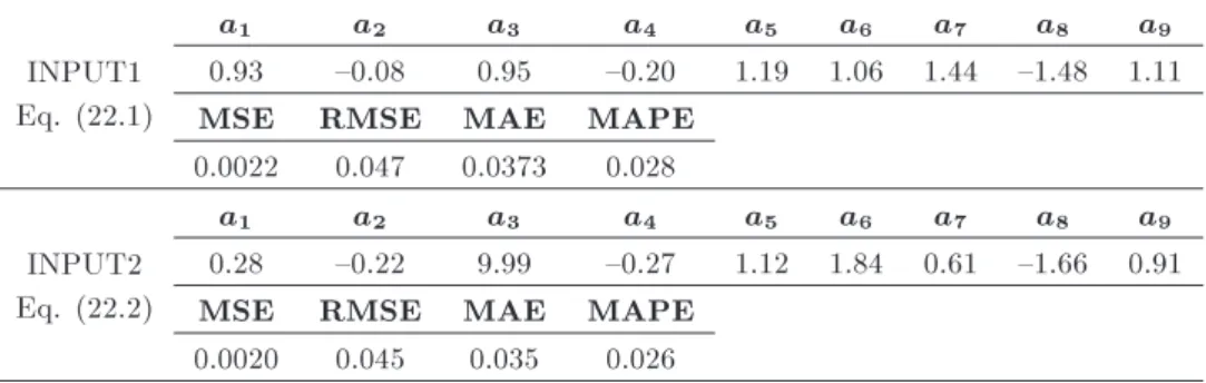
Table 6. Characteristics and statistical errors of Eqs. (22.1) and (22.2). INPUT1
Eq. (22.1)
a1 a2 a3 a4 a5 a6 a7 a8 a9
0.93 {0.08 0.95 {0.20 1.19 1.06 1.44 {1.48 1.11
MSE RMSE MAE MAPE
0.0022 0.047 0.0373 0.028 INPUT2
Eq. (22.2)
a1 a2 a3 a4 a5 a6 a7 a8 a9
0.28 {0.22 9.99 {0.27 1.12 1.84 0.61 {1.66 0.91
MSE RMSE MAE MAPE
0.0020 0.045 0.035 0.026
power (a9, a7, a5, a3) were considered. As was the
case with previous equations, one constant value (a1)
was considered for all of the equations. Then, a1 to
a9 were calculated with the PSO algorithm, and the
optimization results and MSE values for INPUT1 and INPUT2 are given in Table 6 as Eqs. (22.1) and (22.2). As with other previous equations, the error value was lower in INPUT2. The interesting point here is that the error value was at its minimum compared with other equations. Since the shape of Eq. (22) is simple and standard, it can model the discharge coecient (CM)
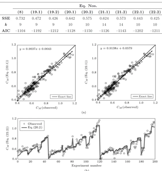
of a modied triangular side weir coecient with an insignicant error. Figure 7(a) shows that this equation reduces the error to a minimum; however, the t and
exact lines do not overlap as they do in Eq. (20.2). A comparison of Figure 5(b) with Figure 7(b) shows that Eq. (20.2) has more ecient performance than Eq. (22.2) for experiment numbers 0 to 40, while Eq. (22.2) has higher accuracy with respect to the other experiment numbers. A comparison of Figure 4(b) with Figure 7(b) shows that both models are too weak to model experiment numbers 0 to 40; however, Eq. (19.2) functions better in areas where CM experiences sudden
changes (experiment numbers 100 to 120):
CM =a1+ a2(Var1)a3+ a4(Var2)a5+ a6(Var3)a7
Table 7. AIC amounts for the considered models. Eq. Nos.
(8) (19.1) (19.2) (20.1) (20.2) (21.1) (21.2) (22.1) (22.2) SSE 0.732 0.472 0.426 0.642 0.575 0.624 0.573 0.443 0.425
k 9 9 9 10 10 14 14 10 10
AIC {1104 {1192 {1212 {1128 {1150 {1126 {1143 {1202 {1211
Figure 7. (a) Scatter plot of comparing observed CM and the estimated CM by Eqs. (22.1) and (22.2). (b) Comparison
of the observed CM and the estimated CM by Eq. (22.2).
4.5. Akaike Information Criterion (AIC) By adding parameters to the model constantly, it may work somewhat better; however, overtting and information loss concerning the real pattern may occur. Therefore, AIC [50-52] represents a trade-o between the number of parameters involved in the model and the increase or decrease of error. AIC is used to select a model by considering not only the error, but also the number of parameters used to develop the model. By assuming that the errors are normally distributed in the model, AIC equation is obtained as follow:
AIC = n log
SSE n
+ 2k; (23)
where n is the number of observations, k is the number of used parameters used in the model plus one, and SSE is the Sum of Squared Errors of the model.
The parameters used in this equation for the models developed in the present study are shown in Table 7.
According to AIC formulation, the model enjoy-ing a better t has lower AIC value. Based on Tables 3 and 6, Eq. (22.2) with RMSE of 0.045 performed somewhat better than the Eq. (19.2) with RMSE of 0.049 did. However, Table 7 shows that the number of involved parameters of Eq. (22.2) is more than that of Eq. (19.2)'s parameters. Therefore, Eq. (19.2) with AIC of {1212 has the best-t score according to this criterion.
5. Conclusions
In this research, a PSO model was developed to deter-mine the discharge coecients of modied triangular side weirs. Two hundred experimental datasets were used for the PSO model. Four dierent equation forms
were used to determine the most accurate form; in each form, two non-dimensional parameters were used as inputs to the PSO model. As shown, the second input series provided more accurate results and included w=L (weir height/weir length), Fr1=sine(0) (upstream
Froude number/sine (weir included angle/2)), w=Y1
(weir height/upstream ow depth), and wsine(0)=Y 1
((weir included angle/2)/upstream ow depth). The equations based on the PSO algorithm were compared with a nonlinear regression model, and it was found that they were more accurate than the regression mod-els. After comparing four forms of the equations used in this study, it was determined that the performance of the power equation is better than those of the other forms are. It also was determined that a combination of the PSO algorithm with a power equation could be used successfully to compute the discharge coecients of modied triangular side weirs.
References
1. De Marchi, G. \Lateral weirs fundamentals" [Saggio di teoria del funzionamento degli stramazzi laterali, L'Energia Elettrica. (In Italian), 11(11), pp. 849-860 (1934).
2. Ackers, P. \A theoretical consideration of side-weirs as storm water overows", Pros. ICE, 6, pp. 250-269 (1957).
3. Yu-Tech, L. \Discussion of spatially varied ow over side weir", Journal of Hydrologic Engineering, 98(11), pp. 2046-2048 (1972).
4. Singh, R., Manivannan, D., and Satyanarayana, T. \Discharge coecient of rectangular side weirs", Jour-nal of Irrigation and Drainage Engineering, 120(4), pp. 814-819 (1994).
5. Swamee, P.K., Pathak, S.K., and Ali, M.S. \Side-weir analysis using elementary discharge coecient", Jour-nal of Irrigation and Drainage Engineering, 120(4), pp. 742-755 (1994).
6. Ura, M., Kita, Y., Akiyama, J., Moriyama, H., and Kumar, J.A. \Discharge coecient of oblique side-weirs", Journal of Hydroscience and Hydraulic Engi-neering, 19(1), pp. 85-96 (2001).
7. Borghei, S.M. and Parvaneh, A. \Discharge charac-teristics of a modied oblique side weir in subcritical ow", Flow Measurement and Instrumentation, 22(5), pp. 370-376 (2011).
8. Najafzadeh, M. and Barani, G.A. \Comparison of group method of data handling based genetic program-ming and back propagation systems to predict scour depth around bridge piers", Scientia Iranica, 18(6), pp. 1207-1213 (2011).
9. Najafzadeh, M. and Azamathulla, H.M. \Group method of data handling to predict scour depth around bridge piers", Neural Computing and Applications, 23(7), pp. 2107-2112 (2013).
10. Najafzadeh, M., Barani, G.-A., and Hessami Kermani, M.R. \GMDH based back propagation algorithm to predict abutment scour in cohesive soils", Ocean En-gineering, 59, pp. 100-106 (2013).
11. Najafzadeh, M., Barani, G.-A., and Hessami-Kermani, M.-R. \Group method of data handling to predict scour at downstream of a ski-jump bucket spillway", Earth Science Informatics, 7(4), pp. 231-248 (2014). 12. Najafzadeh, M. and Lim, S.Y. \Application of
im-proved neuro-fuzzy GMDH to predict scour depth at sluice gates", Earth Science Informatics, 8(1), pp. 187-196 (2015).
13. Najafzadeh, M. \Neuro-fuzzy GMDH based particle swarm optimization for prediction of scour depth at downstream of grade control structures", Engineering Science and Technology, an International Journal, 18(1), pp. 42-51 (2015).
14. Grace, J.L. and Priest, M.S., Division of Flow in Open Channel Junctions, Engineering Experiment Station, Alabama Polytechnic Institute (1958).
15. More, J. \The Levenberg-Marquardt algorithm: Im-plementation and theory", Watson, G.A. (Ed.) In Numerical Analysis, pp. 105-116, Springer Berlin Hei-delberg (1978).
16. Chau, K., Wu, C., and Li, Y. \Comparison of several ood forecasting models in Yangtze River", Journal of Hydrologic Engineering, 10(6), pp. 485-491 (2005). 17. Cheng, C., Chau, K., Sun, Y., and Lin, J. \Long-Term
Prediction of Discharges in Manwan Reservoir Using Articial Neural Network Models", Wang, J., Liao, X.F., and Yi, Z. (Eds.), In Advances in Neural Networks -ISNN 2005, pp. 1040-1045, Springer Berlin Heidelberg (2005).
18. Chen, W. and Chau, K. \Intelligent manipulation and calibration of parameters for hydrological models", International Journal of Environment and Pollution, 28(3), pp. 432-447 (2006).
19. Firat, M. and Gungor, M. \Hydrological time-series modelling using an adaptive neuro-fuzzy inference system", Hydrological Processes, 22(13), pp. 2122-2132 (2008).
20. Wu, C., Chau, K., and Li, Y. \Predicting monthly streamow using data-driven models coupled with data-preprocessing techniques", Water Resources Re-search, 45(8), p. W08432 (2009).
21. Asadi, S., Shahrabi, J., Abbaszadeh, P., and Taban-mehr, S. \A new hybrid articial neural networks for rainfall-runo process modeling", Neurocomputing, 121, pp. 470-480 (2013).
22. Yurtseven, I. and Zengin, M. \Neural network mod-elling of rainfall interception in four dierent forest stands", Annals of Forest Research, 56(2), pp. 351-362 (2013).
23. Muttil, N. and Chau, K.-W. \Neural network and genetic programming for modelling coastal algal blooms", International Journal of Environment and Pollution, 28(3), pp. 223-238 (2006).
24. Kisi, O. and Ozturk, O. \Adaptive neurofuzzy computing technique for evapotranspiration estima-tion", Journal of Irrigation and Drainage Engineering, 133(4), pp. 368-379 (2007).
25. Cobaner, M. \Evapotranspiration estimation by two dierent neuro-fuzzy inference systems", Journal of Hydrology, 398(3), pp. 292-302 (2011).
26. Hager, W.H. \Discussion of separation zone at open-channel junctions", Journal of Hydraulic Engineering, 113(4), pp. 539-543 (1987).
27. Najafzadeh, M. and Tafarojnoruz, A. \Evaluation of neuro-fuzzy GMDH-based particle swarm optimization to predict longitudinal dispersion coecient in rivers", Environmental Earth Sciences, 75(2), p. 157 (2016). 28. Maanen, B.V., Coco, G., Bryan, K.R., and Ruessink,
B. \The use of articial neural networks to analyze and predict alongshore sediment transport", Nonlinear Processes in Geophysics, 17(5), pp. 395-404 (2010). 29. Ebtehaj, I. and Bonakdari, H. \Evaluation of sediment
transport in sewer using articial neural network", Engineering Applications of Computational Fluid Me-chanics, 7(3), pp. 382-392 (2013).
30. Taormina, R., Chau, K.-W., and Sethi, R. \Articial neural network simulation of hourly groundwater levels in a coastal aquifer system of the Venice lagoon", En-gineering Applications of Articial Intelligence, 25(8), pp. 1670-1676 (2012).
31. Pulido-Calvo, I. and Gutierrez-Estrada, J.C. \Im-proved irrigation water demand forecasting using a soft-computing hybrid model", Biosystems Engineer-ing, 102(2), pp. 202-218 (2009).
32. Tiwari, M.K. and Adamowski, J. \Urban water de-mand forecasting and uncertainty assessment using ensemble wavelet-bootstrap-neural network models", Water Resources Research, 49(10), pp. 6486-6507 (2013).
33. Najafzadeh, M. and Sattar, A.M.A. \Neuro-fuzzy GMDH approach to predict longitudinal dispersion in water networks", Water resources management, 29(7), pp. 2205-2219 (2015).
34. Bilhan, O., Emin Emiroglu, M., and Kisi, O. \Appli-cation of two dierent neural network techniques to lateral outow over rectangular side weirs located on a straight channel", Advances in Engineering Software, 41(6), pp. 831-837 (2010).
35. Kisi, O., Emin Emiroglu, M., Bilhan, O., and Gu-ven, A. \Prediction of lateral outow over triangular labyrinth side weirs under subcritical conditions using soft computing approaches", Expert Systems with Ap-plications, 39(3), pp. 3454-3460 (2012).
36. Emin Emiroglu, M., Kisi, O., and Bilhan, O. \Pre-dicting discharge capacity of triangular labyrinth side weir located on a straight channel by using an adap-tive neuro-fuzzy technique", Advances in Engineering Software, 41(2), pp. 154-160 (2010).
37. Bilhan, O., Emiroglu, M.E., and Kisi, O. \Use of articial neural networks for prediction of discharge coecient of triangular labyrinth side weir in curved channels", Advances in Engineering Software, 42(4), pp. 208-214 (2011).
38. Emiroglu, M.E., Bilhan, O., and Kisi, O. \Neural net-works for estimation of discharge capacity of triangular labyrinth side-weir located on a straight channel", Expert Systems with Applications, 38(1), pp. 867-874 (2011).
39. Neary, V. and Sotiropoulos, F. \Numerical investiga-tion of laminar ows through 90-degree diversions of rectangular cross-section", Computers & Fluids, 25(2), pp. 95-118 (1996).
40. Khorchani, M. and Blanpain, O. \Development of a discharge equation for side weirs using articial neural networks", Journal of Hydroinformatics, 7, pp. 31-39 (2005).
41. Dursun, O.F., Kaya, N., and Firat, M. \Estimating discharge coecient of semi-elliptical side weir using ANFIS", Journal of Hydrology, 426, pp. 55-62 (2012). 42. Bagheri, S., Kabiri-Samani, A., and Heidarpour, M. \Discharge coecient of rectangular sharp-crested side weirs, Part I: Traditional weir equation", Flow Mea-surement and Instrumentation, 35, pp. 109-115 (2013). 43. Kennedy, J. and Eberhart, R. \Particle swarm opti-mization", Proceedings of IEEE international confer-ence on neural networks, Perth, Australia, pp. 1942-1948 (1995).
44. Tripathi, P.K., Bandyopadhyay, S., and Pal, S.K. \Multi-objective particle swarm optimization with time variant inertia and acceleration coecients", In-formation Sciences, 177(22), pp. 5033-5049 (2007). 45. Chatterjee, A. and Siarry, P. \Nonlinear inertia weight
variation for dynamic adaptation in particle swarm op-timization", Computers & Operations Research, 33(3), pp. 859-871 (2006).
46. Helton, J., Iman, R., Johnson, J., and Leigh, C. \Uncertainty and sensitivity analysis of a model for multicomponent aerosol dynamics", Nuclear Technol-ogy, 73(3), pp. 320-342 (1986).
47. Iman, R.L. and Helton, J.C. \An investigation of uncertainty and sensitivity analysis techniques for computer models", Risk Analysis, 8(1), pp. 71-90 (1988).
48. Downing, D.J., Gardner, R., and Homan, F. \An ex-amination of response-surface methodologies for uncer-tainty analysis in assessment models", Technometrics, 27(2), pp. 151-163 (1985).
49. Hamby, D.M. \A review of techniques for parameter sensitivity analysis of environmental models", Envi-ronmental Monitoring and Assessment, 32(2), pp. 135-154 (1994).
50. Akaike, H. \Information theory and an extension of the maximum likelihood principle", Kotz, S. and Johnson, N.L. (Eds.), In Breakthroughs in Statistics: Foundations and Basic Theory, pp. 610-624, Springer New York, New York, NY (1992).
51. Akaike, H. \A new look at the statistical model iden-tication", IEEE Transactions on Automatic Control, 19(6), pp. 716-723 (1974).
52. Akaike, H. \Prediction and entropy", Atkinson, A.C. and Fienberg, S.E. (Eds.), In A Celebration of Statis-tics: The ISI Centenary Volume A Volume to Cel-ebrate the Founding of the International Statistical Institute in 1885, pp. 1-24, Springer New York, New York, NY (1985).
Biographies
Amir Hossein Zaji is now a PhD Student in Hy-draulic Structures (Civil Engineering), Department of Civil Engineering, University of Razi, Kermanshah, Iran. He has 20 published papers in ISI journals. He works in the eld of soft computing methods in engineering applications. He has been rated as a distinguished researcher in Razi University, 2015. Hossein Bonakdari is a Professor at the Department of Civil Engineering of University of Razi Univer-sity; he earned his PhD in Civil Engineering at the University of Caen-France. After obtaining PhD, Dr. Bonakdari joined University of Razi as a faculty member in 2006; presently, he is a Professor at the Department of Civil Engineering. He has supervised 5 PhD and 30 MS theses. He enjoys brilliant teaching experience of more than 16 years in the eld of Civil Engineering. Furthermore, From 2013 till 2015, he was the Director General of Training, Research and
Technology Development at Ministry of Energy, Iran and also the Deputy of Planning & Development in National Water and Wastewater Engineering Com-pany, Iran, from 2011-2013. His elds of special-ization and interest include practical application of soft computing in engineering, modeling of wastewater urban drainage systems, sediment transport, com-putational uid dynamic and hydraulics, design of hydraulic structures and uid mechanics. From 2010 till 2011, he has been a researcher at Laboratory of Civil and Environmental Engineering, INSA of Lyon, France. Results obtained from his researches have been published in more than 100 papers in international journals (h-index=13). He has also more than 150 presentations in national and international conferences. He published two books. He has been rated as a distinguished researcher in Razi University, 2014, 2015 and 2016.
Shahaboddin Shamshirband is now a Senior Lec-turer at the Department of Computer System and Technology, University of Malaya. He received his MSc degree in Computer Science from Islamic Azad Univer-sity of Mashhad (IAUM), Iran in 2006. He joined the Faculty of Computer Science, Islamic Azad University, Iran for seven years. Currently, he is pursuing his PhD from the University of Malaya, Malaysia. He is working in a multi-disciplinary environment involving applications of computational intelligence and neuro-computing in Civil Engineering. He has published more than one hundred papers in ISI journals.
![Table 1. Interval variations in experimental tests of Borghei and Parvaneh [7].](https://thumb-us.123doks.com/thumbv2/123dok_us/8374772.2224460/3.892.163.751.177.569/table-interval-variations-experimental-tests-borghei-parvaneh.webp)