Aliasing, Image Sampling
and Reconstruction
Many of the slides are taken from Thomas Funkhouser course slides and the rest from various sources over the web…
Recall: a pixel is a point…
• It is NOT a box, disc or teeny wee light
• It has no dimension
• It occupies no area
• It can have a coordinate
•
More
than a point, it is a
SAMPLE
Image Sampling
• An image is a 2D rectilinear array of samples
oQuantization due to limited intensity resolution oSampling due to limited spatial and temporal resolutionPixels are
infinitely small
point samples
Imaging devices area sample.
• In video camera the CCD array is an area integral over a pixel.
• The eye: photoreceptors
Intensity, I
J. Liang, D. R. Williams and D. Miller, "Supernormal vision and high- resolution retinal imaging through adaptive optics," J. Opt. Soc. Am. A 14, 2884- 2892 (1997)
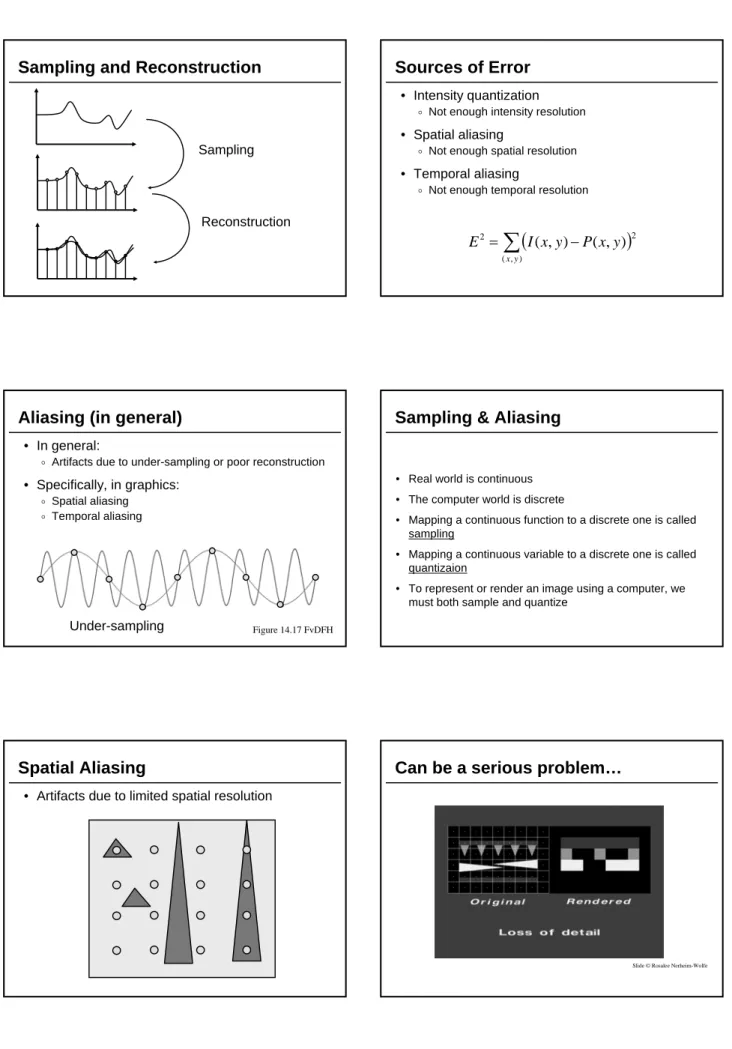
Sampling and Reconstruction
Figure 19.9 FvDFH Slide © Rosalee Nerheim-Wolfe
Sampling and Reconstruction
Sampling
Reconstruction
Sources of Error
• Intensity quantization
o Not enough intensity resolution
• Spatial aliasing
o Not enough spatial resolution
• Temporal aliasing
o Not enough temporal resolution
(
)
∑
−
=
) , (
2 2
)
,
(
)
,
(
y xy
x
P
y
x
I
E
Aliasing (in general)
• In general:
oArtifacts due to under-sampling or poor reconstruction
• Specifically, in graphics:
oSpatial aliasing oTemporal aliasing
Figure 14.17 FvDFH
Under-sampling
Sampling & Aliasing
• Real world is continuous • The computer world is discrete
• Mapping a continuous function to a discrete one is called sampling
• Mapping a continuous variable to a discrete one is called quantizaion
• To represent or render an image using a computer, we must both sample and quantize
Spatial Aliasing
• Artifacts due to limited spatial resolution
Slide © Rosalee Nerheim-Wolfe
Spatial Aliasing
• Artifacts due to limited spatial resolution
“Jaggies”
Temporal Aliasing
• Artifacts due to limited temporal resolution
o Strobingo Flickering
Temporal Aliasing
• Artifacts due to limited temporal resolution
oStrobingoFlickering
Temporal Aliasing
• Artifacts due to limited temporal resolution
o Strobingo Flickering
Temporal Aliasing
• Artifacts due to limited temporal resolution
oStrobingoFlickering
The raster aliasing effect – removal is called
antialiasing
Images by Don Mitchell
Nearest neighbor sampling
Filtered Texture:
Blurring doesn’t work well.
Removed the jaggies, but also all the detail ! →Reduction in resolution
Unweighted Area Sampling
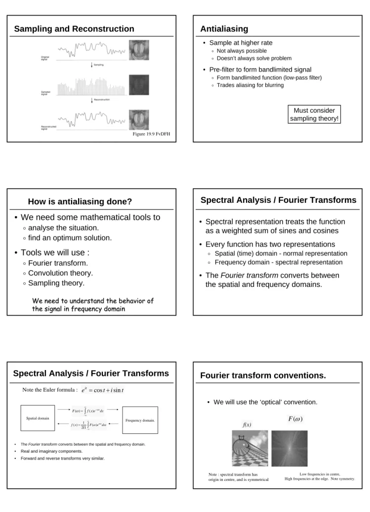
Sampling and Reconstruction
Figure 19.9 FvDFH
Antialiasing
• Sample at higher rate
o Not always possible
o Doesn’t always solve problem
• Pre-filter to form bandlimited signal
o Form bandlimited function (low-pass filter) o Trades aliasing for blurring
Must consider
sampling theory!
How is antialiasing done?
• We need some mathematical tools to
o
analyse the situation.
o
find an optimum solution.
• Tools we will use :
o
Fourier transform.
o
Convolution theory.
o
Sampling theory.
We need to understand the behavior of
We need to understand the behavior of
the signal in frequency domain
the signal in frequency domain
Spectral Analysis / Fourier Transforms
• Spectral representation treats the function
as a weighted sum of sines and cosines
• Every function has two representations
o
Spatial (time) domain - normal representation
o
Frequency domain - spectral representation
• The Fourier transform converts between
the spatial and frequency domains.
Spectral Analysis / Fourier Transforms
• The Fourier transform converts between the spatial and frequency domain. • Real and imaginary components.
• Forward and reverse transforms very similar.
Spatial domain Frequency domain.
∫ ∞
∞ −
− = fxe dx F(ω) () iωx
∫
∞
∞ − Π = Fωeωdω
x
f ()ix
2 1 ) (
t i t eit=cos + sin
Note the Euler formula :
Fourier transform conventions.
• We will use the ‘optical’ convention.
f(x)
F
(
ω
)
Note : spectral transform has origin in centre, and is symmetrical
Low frequencies in centre, High frequencies at the edge. Note symmetry.
Sampling Theory
• How many samples are required to represent a
given signal without loss of information?
• What signals can be reconstructed without loss
for a given sampling rate?
Spectral Analysis
• Spatial domain:
o Function: f(x) o Filtering: convolution
• Frequency domain:
oFunction: F(u) oFiltering: multiplicationAny signal can be written as a sum of periodic functions.
1-D Fourier
Transform
• Makes any signal
I
(
x
) out of sine
waves
• Converts spatial domain into
frequency domain
• Yields spectrum
F
(
u
) of frequencies
u
ouis actually complex
oOnly worried about amplitude: |u|
• DC term:
F
(0) = mean
I
(
x
)
• Symmetry:
F
(-
u
) =
F
(
u
)
∫
∫
= − = du jux u F x I dx jux x I u F ) exp( ) ( 2 1 ) ( ) exp( ) ( 2 1 ) ( π π ) / arctan( arg sin cos ) exp( 1 2 2 2 a b bj a b a bj a ux j ux jux j = + + = + − = − − = I x F u 0 p 1/p Spatial FrequencyFourier Transform
Figure 2.6 Wolberg
Fourier Transform
Figure 2.5 Wolberg
Sampling Theorem
• A signal can be reconstructed from its samples,
if the original signal has no frequencies
above 1/2 the sampling frequency - Shannon
• The minimum sampling rate for bandlimited
function is called “Nyquist rate”
A signal is bandlimited if its highest frequency is bounded. The frequency is called the bandwidth.
Convolution
• Convolution of two functions (= filtering):
• Convolution theorem
oConvolution in frequency domain is same as multiplication in spatial domain, and vice-versa
∫
∞ ∞ −
−
=
⊗
=
f
x
h
x
f
λ
h
x
λ
d
λ
x
g
(
)
(
)
(
)
(
)
(
)
Antialiasing in Image Processing
• General Strategy
o Pre-filter transformed image via convolution with low-pass filter to form bandlimited signal
• Rationale
o Prefer blurring over aliasing
Filtering in the frequency domain
Image Frequency domain Filter Image Fourier
Transform
Fourier Transform
Lowpass filter
Highpass filter
Low and High Pass Filtering.
• Low pass
• High pass
Product and Convolution
• Product of two functions is just theirproduct at each point
• Convolution is the sum of products of one function at a point and the other function at all other points
• E.g. Convolution of square wave with square wave yields triangle wave • Convolution in spatial domain is product in
frequency domain, and vice versa
f*g
Ù
FG
fg
Ù
F*G
∫
−= gshx sds x
h
g* )( ) () ( ) (
) ( ) ( ) )(
(gh x =gxhx
Filtering in the space domain
• Blurring or averaging pixels together.
Calculate integral of one function, f(x) by a sliding second function g(x-y). Known as Convolution.
∫
−
=
⊗
=
f
g
f
x
g
x
y
dy
x
h
(
)
(
)
(
)
g(y)
Increment x
h(x) Integrate
over y f(x)
Low-pass Filtering
Sampling Functions
• Sampling takes measurements of a continuous function at discrete points • Equivalent to product of continuous
function and sampling function • Uses a sampling function s(x) • Sampling function is a collection of
spikes
• Frequency of spikes corresponds to their resolution
• Frequency is inversely proportional to the distance between spikes
• Fourier domain also spikes • Distance between spikes is the
frequency
p
1/p s(x)
S(u) Spatial Domain
Frequency Domain
Sampling , the Comb function
How can we represent sampling ?
Multiplication of the sample with a regular train of delta functions.
Sampling: Frequency domain.
The Fourier transform of regular comb of delta functions is a comb.
Spacing is inversely proportional
Multiple solutions at regularly increasing values of f
Reconstruction in frequency domain
Bandpass filter due to regular array of pixels.
Original signal.
Undersampling leads to aliasing.
Spurious components : Cause of aliasing. Samples are too close
together in f.
Sampling
p 1/p
I(x)
s(x)
(Is)(x)
(Is’)(x)
s’(x)
F(u)
S(u)
(F*S)(u)
S’(u)
(F*S’)(u)
Aliasing, can’t retrieve original signal
Shannon’s Sampling Theorem
• Sampling frequency needs to be atleast twice the highest signal frequency • Otherwise the first replica interferes
with the original spectrum • Sampling below this Nyquist limit
leads to aliasing
• Conceptually, need one sample for each peak and another for each valley
max {u : F(u) > ε}
p > 2 max u
The Sampling Theorem.
A signal can be reconstructed from its samples without loss of information, if the original signal
has no frequencies above 1/2 the sampling frequency
For a given bandlimited function, the rate at which it must be sampled is called the Nyquist Frequency
This result is known as the Sampling Theorem
Prefiltering
• Aliases occur at high frequencies – Sharp features, edges – Fences, stripes, checkerboards • Prefiltering removes the high frequency
components of an image before it is sampled
• Box filter (in frequency domain) is an ideal low pass filter
– Preserves low frequencies – Zeros high frequencies • Inverse Fourier transform of a box
function is a sinc function sinc(x) = sin(x)/x
• Convolution with a sinc function removes high frequencies
DC Term
Spatial Domain
Frequency Domain sinc(x)
I(x) F(u)
(I*sinc)(x) (Fbox)(u) box(u)
Prefiltering Can Prevent Aliasing
(Is’)(x)
s’(x) S’(u)
(F*S’)(u)
I’ = (I*sinc)
(F’*S’)(u) (I’s’)(x)
F’ = (F box)
(box)(F’*S’)(u)
(sinc)*(I’s’)(x)
Aliasing in the space domain.
Original signal
Aliased result
Summary :Aliasing is the appearance of spurious signals when the frequency of the input signal goes above the Nyquist limit.
Sampling at the Nyquist Frequency
Sampling Below the Nyquist Frequency
How do we remove aliasing ?
• Perfect solution - prefilter with perfect bandpass filter.
Perfect bandpass
No aliasing. Aliased example
How do we remove aliasing ?
• Perfect solution - prefilter with perfect bandpass filter. o Difficult/Impossible to do in frequency domain. • Convolve with sinc function in space domain
o Optimal filter - better than area sampling. o Sinc function is infinite !!
o Computationally expensive.
• Cheaper solution : take multiple samples for each
pixel and average them together →supersampling.
• Can weight them towards the centre →weighted
average sampling • Stochastic sampling
Removing aliasing is called
antialiasing
How do we remove aliasing ?
The ‘Sinc’ function.
∫
∫
∞ ∞
− −
− − =1/2
2 / 1
)
(xe dx e dx square iωx iωx
ω ω ω ω ω ω ω ω 2 1 2 1 sin 2 1 2 1 2 1 2 1 2 1 2 1 = + − = − = − − − i i e e x i e i i x i t i t eit sin cos + =
The Sinc Filter
Common Filters
Sample-and-Hold
Image Reconstruction
• Re-create continuous image from samples
o Example: cathode ray tube
Image is reconstructed
by displaying pixels
with finite area
(Gaussian)
End…
Adjusting Brightness
• Simply scale pixel components
o Must clamp to range (e.g., 0 to 255)Adjusting Contrast
• Compute mean luminance for all pixels
oluminance = 0.30*r + 0.59*g + 0.11*b• Scale deviation from for each pixel component
oMust clamp to range (e.g., 0 to 255)Original More Contrast
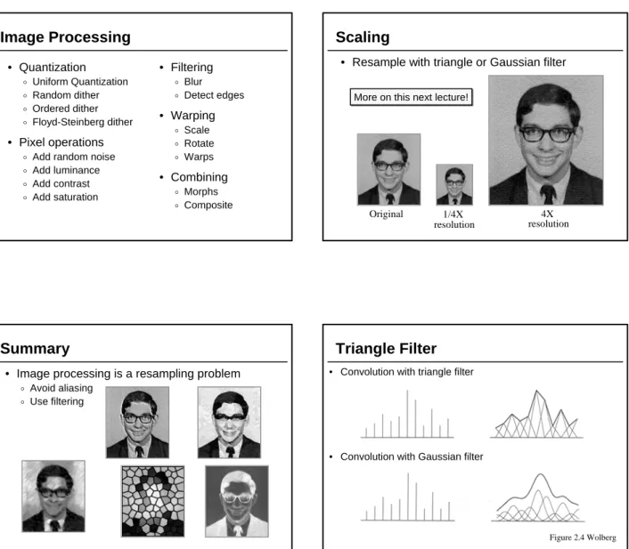
Image Processing
• Consider reducing the image resolution
Original image 1/4 resolution
Image Processing
Resampling
• Image processing is a resampling problem
Thou shalt avoid aliasing!
Image Processing
• Quantization
oUniform Quantization
oRandom dither
oOrdered dither oFloyd-Steinberg dither
• Pixel operations
oAdd random noise
oAdd luminance
oAdd contrast oAdd saturation
• Filtering
o Bluro Detect edges
• Warping
o Scale o Rotate o Warps• Combining
o Morphs o CompositeAdjust Blurriness
• Convolve with a filter whose entries sum to one
oEach pixel becomes a weighted average of its neighborsOriginal Blur ⎥ ⎥ ⎥ ⎥ ⎦ ⎤ ⎢ ⎢ ⎢ ⎢ ⎣ ⎡ 16 1 16 2 16 1 16 2 16 4 16 2 16 1 16 2 16 1 Filter =
Edge Detection
• Convolve with a filter that finds differences
between neighbor pixels
Original Detect edges
⎥ ⎥ ⎦ ⎤ ⎢ ⎢ ⎣ ⎡ − − − + − − − − − 1 1 1 1 8 1 1 1 1 Filter =
Image Processing
• Quantization
o Uniform Quantization
o Random dither
o Ordered dither o Floyd-Steinberg dither
• Pixel operations
o Add random noise
o Add luminance
o Add contrast o Add saturation
• Filtering
o Bluro Detect edges
• Warping
o Scale
o Rotate
o Warps
• Combining
o Morphs
o Composite
Scaling
• Resample with triangle or Gaussian filter
Original 1/4X resolution
4X resolution
More on this next lecture!
Summary
• Image processing is a resampling problem
oAvoid aliasingoUse filtering
Triangle Filter
• Convolution with triangle filter
Figure 2.4 Wolberg • Convolution with Gaussian filter