Northeastern University

(1)

(2)

Northeastern University

Master’s Thesis Proposal

CS 7990

Word-vector Regularization for text classification

algorithms

Author:

Ramkishan Panthena

Advisor:

Dr. Virgil Pavlu

Official Reader:

Dr. Byron Wallace

(3)

Abstract

A simple and efficient baseline for text classification is to represent sentences as bag-of-words (BoW) and train a linear classifier. The bag-of-words model is simple to implement and offers flexibility for customization by providing differ-ent scoring techniques for user specific text data. In many problem domains, these linear classifiers are preferred over more complex models like CNN, LSTM because of their efficiency, robustness and interpretability.

However, a large vocabulary can cause extremely sparse representations which are harder to model, where the challenge is for models to harness very little information in such a large representational space. Also, these classifi-cation problems are categorized by large number of classes and highly imbal-anced distribution of data across these classes. In such cases, the traditional linear classifiers would treat each word separately and assign them different coefficients based on the frequency in which they occur in the train set. This would result in lower test accuracy when it comes across instances where a word which was occurring less frequently in the train set, occurs more often in the test set.

Our thesis aims to solve this problem by constraining weights of rare fea-tures by similar, more frequent ones, using semantic similarity. This would enforce similar words to have similar weights thereby improving model perfor-mance. Thus, based on how similar two features are, our proposed model can improve the feature importance of a sparse word by increasing its regression co-efficient, thereby improving the test accuracy in the above mentioned sce-nario.

(4)

Chapter 1 Introduction

The goal of text classification is to classify text documents into one or more classes according to their content. For this purpose, a document must be transformed into a representation which is suitable for the learning algorithm and the classification task. Representing documents as bag-of-words is a com-monly used method in document classification where the frequency of occur-rence of each word is used as a feature for training a classifier. However, one should note that when using this representation, some document information is lost as the model disregards grammar and word ordering.

1.1 Problem Statement

Although the bag-of-words model is widely used and performs exceptionally well in most text classification problems, it contains several limitations. As per Zipf’s law [1], given a large sample of words used, the frequency of any word is inversely proportional to its rank in the frequency table. So, word number n has a frequency proportional to 1/n. Thus, a large vocabulary can cause extremely sparse representations.

The classification accuracy we observe on the test set largely depends on the quality of training sets we have used to build our models. That is, if the training information is sparse, then we can expect the category model to be a poor representation of a category thereby leading to poor classification accuracy. Words that occur rarely do not give a learning algorithm enough information to determine its influence on classification correctly.

Thus, in such a case any linear classifier like logistic regression, naive bayes, linear SVM would treat each word independently and assign them different co-efficients based on the impact of the individual word on the response variable. As the training data for rare words would be sparse, their coefficients would be near 0 implying that the impact of these features is small. This may not be the case as these rare words might be misrepresented due to sparse data. Our model tries to solve this problem by using a word-vector regularizer that as-signs similar coefficients to words which are used in a similar context, thereby boosting the effect of similar but rare features on the final prediction.

We use logistic regression for binary text classification on a bag-of-words model. Let θ(i) be the regression coefficients of wordi which determines the

(7)

association between each feature value (word occurrence in document) and what the target we are trying to predict.

The cost function for logistic regression would be given as: Cost(h(θ)(x), y) =

(

−log(h(θ)(x)), if y=1

−log(1−h(θ)(x)),if y=0

(1.1)

In general, the features with larger coefficients are more important because they make a significant contribution in predicting the correct class. However if a wordk is rare, its corresponding regression coefficient (θ(k)) could be very

small or very large (minimizing the loss) due to lack of evidence in the training set; which is not useful for predictions. Our plan here is to constrain such coefficients by the word semantic similarity with other more frequent terms, thus simulating a higher occurence and prohibiting extreme behavior. This also helps with non-frequent synonym words in making their coefficients more uniform.

Example: In order to get a better understanding, consider a classification

prob-lem where we are trying to identify whether a document is talking about ani-mals or not. For this example, let’s say we only have five features. The bag-of-words representation using term frequencies for 5 different documents would look like:

dog football canine movies cat

D1 3 0 0 0 4

D2 0 0 0 6 0

D3 5 0 1 0 6

D4 0 8 0 0 0

D5 0 7 0 4 0

Table 1.1: Toy dataset

From the above example, we can see that the word ‘canine’ occurs only once in one of the document. If we train a linear classifier on the above dataset, then ‘canine’ would have a very low feature importance due to its sparse representa-tion. When we test this classifier on a document where ‘canine’ is more densely represented as compared to ‘dog’ or ‘cat’, then that document would get mis-classified as “not talking about animals”.

In contrast, since our model would assign similar weights to similar words and considering ‘dog’ and ‘canine’ are synonyms, our model would assign a higher feature importance to ‘canine’, thereby increasing the probability of making a correct prediction on a new document where ‘canine’ is more densely represented as compared to the train data.

(8)

1.2 Related work

A number of approaches have been proposed to increase the classification ac-curacy on the bag-of-words model.

To aggressively reduce the dimensionality of models, Joachims [2] (1996), Yang and Pedersen[3] (1997) suggested pruning of infrequent words. Mansuy and Hilder [4] (2006) recommended removing of stop words and part-of-speech tags. Porter [5] (1980) proposed removal of suffixes from words. However, Joachims [2] test results revealed that the performance of the system is higher when more words are used as features, with the highest performance achieved using the largest feature set. Any approach that limited the number of words to the most important ones was likely to reduce the classification accuracy as these pruned words lose their ability to contribute to the classification of text. Quinlan [6] (1993) suggested choosing words which have high mutual information with the target concept. However, picking words with high mutual information had relatively poor performance due to its bias towards favoring rare terms, and its sensitivity to probability estimation errors.

In an attempt to address the issue of related concepts in text classification, many researchers have incorporated features using dictionaries and encyclope-dias. Mavroeidis et. al [7] (2005) proposed to extend the traditional bag of words representation by incorporating syntactic and semantic relationships among words using a Word Sense Disambiguation approach. Wang and Domeniconi [8] (2008) explored a similar approach by embedding background knowledge derived from Wikipedia to enrich the representation of documents. Although empirical results have shown improvements in some cases, the applicability of using dictionaries to improve classification accuracy is limited. Ontology is manually built, and the coverage is far too restricted. Recently, Heal et. al [9] (2017) introduced a method for enriching the bag-of-words model by comple-menting rare term information with related terms from Word Vector models. However, it was revealed that these methods achieved significantly better re-sults only when the training sets were small. There wasn’t enough evidence of achieving better results on large datasets.

In addition to incorporating related concepts to improve classification per-formance, other approaches have also been proposed. One of these approaches considers using part-of-speech tags associated with words contained in a doc-ument (Scott and Matwin [10] 1998), (Jensen and Martinez [11] 2000). Since words can have multiple meanings depending upon how and where they are used in a sentence, the part-of-speech may be relevant to text classification. However, a different paper from Mansuy [4] revealed that there was no signifi-cant difference between the accuracy of the classifiers whether part-of-speech tags are utilized or not.

To deal with overfitting, different regularization techniques have also been proposed. Regularization adds a penalty on the different parameters of the model to reduce the freedom of the model. Hence, the model will be less likely to fit the noise and improve its generalization abilities. The Lasso regulariza-tion acts as a way of feature selecregulariza-tion by shrinking some parameters to zero, whereas the Ridge regularization will force the parameters to be relatively small but are not cut to zero.

(9)

Chapter 2 Word-Vectors

Word vectors represent a significant leap forward in advancing our ability to an-alyze relationships across words, sentences, and documents. In doing so, they advance technology by providing machines with much more information about words than has previously been possible using traditional representations of words. It is word vectors that make technologies such as Machine translation, Sentiment analysis, Speech recognition, Question Answering possible.

This chapter will explain the following:

• _{Need for word-embeddings} • _{History of word-embeddings} • Word-vector training

• Semantic Relationship and similarity

• _{Word Pairs and Phrases}

• _{Applications of word embeddings}

• Current advances in word-embeddings

2.1 Need for word-embedding

Traditional NLP systems treated words as atomic units, such as one-hot en-coding and bag-of-words models. These methods used dummy variables to represent the presence or absence of a word in an sentence. For the one-hot encoding, each word is represented by a one-hot vector - a sparse vector in the size of the vocabulary, with 1 representing the presence of a word and 0 representing its absence. The bag-of-words feature vector considers the word occurrence as feature value which is normalized using term frequency and inverse-document frequency to increase the importance of rare words and re-duce the importance of very frequent but less important words like stop words. This choice of word-representation is simple, robust and can act as a good baseline model which can be coded using a few lines of code. It also works very well when your dataset is small and the context is domain specific. However

(10)

these models do not preserve the semantic relationship between words and hence lose important linguistic patterns such as word-order and synonyms. Ex. ”This is good” and ”Is this good” have the same feature representation. They are also difficult to model highly sparse data. Thus, simple scaling up of basic techniques will not result in any significant progress, and we have to focus on more advanced techniques.

2.2 History of word-embeddings

The technique of representing words as vectors has roots in the 1960s with the development of vector space models for information retrieval. Reducing the number of dimensions using singular value decompostitoin led to the in-troduction of latent semantic analysis in the late 1980s. In 2001, Bengio et al. [12] published a paper to tackle language modeling and it was the initial idea of word-embedding. At that time, they named this process as ”learning a distributed representaion for words”.

In 2008, Ronan and Jason [13] introduced a concept of pre-trained model and showed its amazing approach for solving NLP problems. In 2013, a team at Google led by Tomas Mikolov created word2vec [14], a word-embedding toolkit which can train vector space models faster than the previous approaches. Later on, gensim provided an amazing wrapper so that adopt different pre-trained word-embedding models which include Word2Vec (by Google), GloVe [15] (by Stanford), fastText (by Facebook).

2.3 Word-vector training

Training a word2vec model is similar to an autoencoder. We use a simple neural network with a single hideen layer to perform a certain task, but then we’re not going to use it for the task we trained it for. Instead, the goal is to just learn the weights of the hidden layer that are actually the word-vectors that we’re trying to learn.

Training the model is done in one of two ways, either using the context to predict a target word (known as continuous bag of words or CBOW) or using a word to predict a target context, which is called skip-gram. According to Mikolov, the skip-gram model works well with small amount of training data and represents well even rare words or phrases. The CBOW is several times faster to train than the skip-gram and shows slightly better accuracy for the frequent words. Let us first look at the skip gram model.

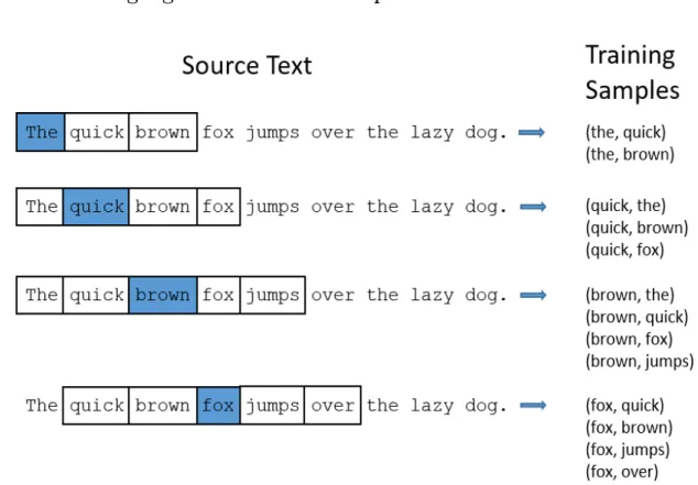
We’re going to train the neural network to do the following: Given a specific word in the middle of a sentence (the input word), look at the nearby words and pick one at random. The network is going to predict the probability for every word in the vocabulary of being the nearby word that we choose. The nearby word is actually a window size parameter to the algorithm. A typical window size might be 5.

The output probabilities indicate how likely is it to find each word near our input word. For example, the input word ”Soviet” will have higher probabilities

(11)

for words like ”Union” and ”Russia” than for unrelated words like ”watermelon” and ”kangaroo”. The neural network will be trained by feeding it word pairs from the train data. The below example shows some of the training samples. The word highlighted in blue is the input word.

Figure 2.1: Training samples for skip-gram model having a window size of 2.

Model details

The words cannot be fed to the neural network as a text string. To do this, we represent the words as a one-hot vector. If we have a vocabulary of 10,000 unique words, then the one-hot vector will have 10,000 components (one for every word in the vocabulary) and we’ll place a 1 in the position corresponding to the word and 0 in all other positions. The output of the network is also a single vector with 10,000 components containing the probability that a ran-domly selected nearby word is that vocabulary word. Thus, the output vector will actually be a probability distribution and not a one-hot vector.

If we want to learn our word-vectors with 300 features, the hidden layer would be represented by a weight matrix with 10,000 rows and 300 columns and the end goal is just to learn the hidden layer weight. The output layer is trained using a softmax regression classifier. The network diagram for both the skip-gram and continuous bag of words models can be seen in the next page.

Improvements to the model

From the previous example, we’ve seen that for word-vectors with 300 com-ponents and 10,000 vocabulary size, both the hidden and output layers will

(12)

Figure 2.2: Skip-gram model: Predicts the surrounding words given the cur-rent word.

Figure 2.3: Continuous Bag of words model: Predicts the current word given the context.

(13)

have the weight matrix of size 300 x 10,000 = 3 million weights each. Running gradient descent on a neural network that large is going to be slow. To address this issue, the word2vec authors addressed this issue in their paper with the following two innovations:

• _{subsampling frequent words to decrease the number of training examples} • _{modifying the optimization objective through ”Negative sampling” which}

causes each training sample to update only a small percentage of model’s weights.

Subsampling Frequent words:

In the previous example of the sentence, ”The quick brown fox jumps over the lazy dog.”, we’ve seen two common problems. Firstly, word pairs like (fox, the) doesn’t tell us much about the meaning of ”fox” as ”the” appears in the context of almost every word. Secondly there are many samples of ”the” than needed to learn a good vector for it. To remediate this, word2vec implements a subsampling scheme that subsamples some of the words from the training data based on its frequency.

Negative Sampling:

Instead of every training sample tweaking all the weights of the neural net-work, we can modify only a small percentage of weights, rather than all of them. With negative [16], we are going to randomly select a small number of negative weights to update along with updating all the positive weights. The negative samples are selected using a unigram distribution, where frequent words are more likely to be selected as negative samples. Thus the probability of picking the word as part of a negative sample to update will depend on the number of times the word appears in the corpus divided by the total number of words in the corpus. This is expressed by the following equation:

P(wi) =

f(wi)

Pn

j=0f(wj)

(2.1) The word vector space implicitly encodes many regularities among words. The resulting distributed representation of words contain a lot of syntactic and semantic information which we will see in the next section.

2.4 Semantic Relationship and Similarity

Word vectors represent words as a vector of real valued numbers where each point captures a dimension of the word’s meaning. Thus, if two different words have very similar ”contexts” i.e., what words are likely to appear around them, then the model needs to output very similar results for these two words. And one way for the network to output similar context predictions for these two words is if the word-vectors are similar. So, if two words have similar contexts,

(14)

then the network will eventually learn similar word vectors for these two words. This means that words such as ”engine” and ”transmission” should have simi-lar word vectors to the word ”car”, whereas the word ”pineapple” should be quite distant. This can also handle stemming for you - the network will likely learn similar word-vectors for words like ”man” and ”men” because these should have similar contexts.

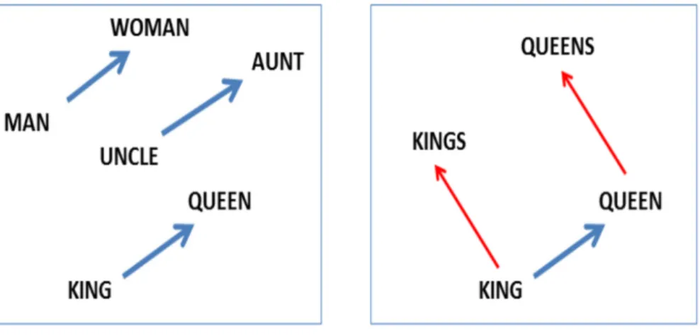
Figure 2.4: The word vector space encodes many regularities among words.

Analogies:

The famous examples that show incredible properties of embeddings is the concept of analogies. We can add and subtract word embeddings and arrive at interesting results. The most famous example is the formula:

• _{”king” - ”man” + ”woman” = ”queen”}

In other words, we can subtract one meaning from the word vector for king (i.e. maleness), add another meaning (femaleness), and show that this new word vector maps closely to the word vector for queen.

2.5 Word Pairs and Phrases

The current implementation of word vectors is limited to its unigram natural behavior. It does not embed bigrams like ”American Airlines” as its whole. In some cases, a word pair like ”Boston Globe” (a newspaper) has a much different meaning than the individual words ”Boston” and ”Globe”. So it makes sense to treat ”Boston Globe” as a single term whenever it occurs when its own word vector representation.

However, the addition of phrases to the model will exponentially increase the vocabulary size. The word2vec team have built a tool that counts the number of times each combination of two words appears in the training text, and use it in an equation to determine which word combinations turn into phrases [17]. The equation is designed to make phrases out of words which occur together often relative to the number of individual occurrences. It also favors phrases

(15)

Figure 2.5: The image shows that we can add and subtract word vectors and it would find the most similar words to the resulting vector.

made of infrequent words in order to avoid making phrases out of common words like ”and the” or ”this is”.

The same word2vec idea can be extended to sentences and complete doc-uments where instead of learning feature representation for words, you learn it for sentences or documents. The applications of these models could depend on the task at hand. A word2vec model can effectively capture semantic rela-tionship between words and hence it can be used to calculate word similarities or fed as features to various NLP tasks such as sentiment analysis, LSTMs etc. However words can only capture so much, there are times when you need rela-tionships between sentences and documents and not just words. For example, if you are trying to figure out if two documents are duplicates of each other.

2.6 Applications of word embeddings

Word embeddings are used in almost all NLP tasks these days:

• _{In conjunction with modelling techniques such as deep neural networks,}

word embeddings have massively improved text classification accuracy in many domains including customer service, spam detection, document classification etc.

• _{Word vectors are also used to build language models which predict the}

next most probable words given the current word. This is learnt through a deep lstm network called Seq2Seq learning. Few applications of these language models are Gmail autoreply and Google search.

• Seq2Seq models with attention gives state of the art accuracy for machine translation.

(16)

Figure 2.6: Machine Translation - English to Spanish. Example showing word vectors having similar structure when trained on comparable corpora

2.7 Current advances in word embeddings

Though pre-trained word embeddings have been very influential, they have a major limitation - they presume that a word’s meaning is stable across sen-tences. However this approach to word representation does not address poly-semy, or the co-existence of many possible meanings for a given word or phrase. There can be cases where there are major differences in meaning for a single word: e.g. get (a verb for obtaining) and get (an animal’s offspring); or bank (a financial institution) and bank (someone to rely on). Also traditional word vectors are a single layer of weights, a shallow representation. Such word vec-tors fail to capture higher-level information that might be even more useful. Recent advances in NLP go from just initializing the first layer of the model to pre-training the entire model with hierarchical representations to make the model capable of performing diverse range of tasks including question answer-ing, natural language inference etc.

Embeddings from Language Models (ELMo)

The motivation for ELMo [18] is that word embeddings should incorporate both word-level characteristics as well as contextual semantics. So instead of taking just the final layer of deep bi-LSTM language model as the word repre-sentation, ELMo embeddings are a function of all internal layers of bi-LSTM. The intutition is that higher level states of the bi-LSTM capture context, while lower level captures syntax. Thus, instead of using a fixed embedding for each word, ELMo looks at the entire sentence before assigning each word an embed-ding thus generating different embedembed-dings for each of its occurence.

(17)

Open AI GPT (Generative Pre-training Transformer)

Open AI GPT [19] is similar to ELMo, with a few differences. Firstly while ELMo uses Bi-LSTMs, GPT is a multi-layer encoder-decoder model with at-tention mechanism. Secondly while ELMo feeds embeddings into models for customized tasks, GPT fine tunes the same base model for all tasks.

However, one drawback of the GPT is its uni-directional nature - the model is only trained to predict the future left-to-right context.

Bidirectional Encoder Representations from Transformers (BERT)

BERT [20] is a direct descendent to GPT — train a large language model on free text and then fine-tune on specific tasks without customized network architectures. Compared to GPT, the largest difference and improvement of BERT is to make training bi-directional. The model learns to predict both context on the left and right. The model architecture of BERT is a multi-layer bi-directional Transformer encoder.

(18)

Chapter 3 Proposed Methods

We propose to enhance the bag-of-words model for text classification by adding additional features to the vanilla logistic regression model. These new features will act as a regularizer which would assign similar coefficients to words used in similar context. We worked on four different implementations detailed below, out of which we found the second one consistently outperforming the other three and also outperforming the comparison baselines.

Obtain word-vectors. Out of the successful deep learning models used for

word-embeddings, two of the most popular ones are Word2Vec [21] and Global Vectors [15]. For our research, we will be using Google’s Word2Vec which has pre-trained word-vectors with 300 dimensions trained using over 100 billion words.

Also it has been seen that a smaller domain specific Word Vector model is modelled better than a general model trained over a much larger corpus of text. Thus Google’s pre-trained Word Vector model which was trained over three million unique words and phrases will be retrained on the training data to generate domain specific Word Vectors.

Train new model. Once the features have been extracted as bag-of-words,

and their corresponding word-vectors retrained, we can train learning models on the cost functions below.

Below is the link to its source code on GitHub. It will be made publicly available upon thesis completion:

https://github.com/RamkishanPanthena/Master-s-Thesis

3.1 M1: Initial word-vector model

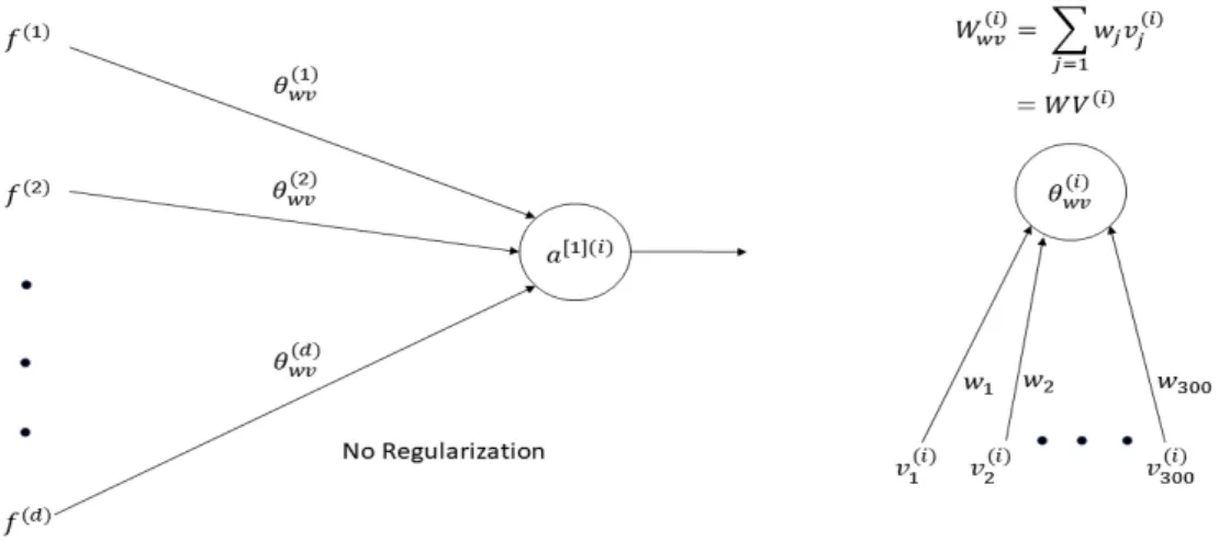
For our initial word-vector model, we built a network where the coefficients are only a function of its word representation (v(i)), without the logistic regression weights, i.e.,

θ(i)=θ_wv(i) _(3.1)

These weights as mentioned in Chapter 3, will be learnt through the word representation of the features using a linear regressor, which will then be passed through a sigmoid/softmax function for classfication i.e.,

(19)

Figure 3.1: Initial word-vectors model

θ(_wvi) =w1v (i) 1 +w2v

(i)

2 +...+wdv

(i)

d = D

X

d=1

w_d(i)v_d(i) _(3.2) where, w= (w1, w2, ..., wd) are the parameters of the regression function.

v = (v1, v2, ..., vd) are d-dimensional word-representations of wordi

Figure 3.2: Comparison of word-vector with CNN model

Comparison with CNN. If we compare the word-vector coefficients model

to a CNN, then this would be similar to a 1D CNN network having one filter, sum pooling and a sigmoid/softmax activation function at the output layer

(20)

with cross entropy loss. We are training on a bag-of-words model which does not consider the order of the sentence, so the kernel size which decides the length of the 1d convolutional window would be 1. Also, from our network we can see that the coefficients are a linear sum of the word-vector representation with no activation layer at the end. To replicate the same on the CNN network, we do not apply an activation function to the single filter. It is directly passed onto the sum pooling layer. This network would then be like the word vector coefficients model.

If our task is multi-class classification, then the model can be seen as a CNN model with N filters and softmax function as the activation function, where N equals to the number of the classes in the dataset. We should change the sum pooling layer to make them work in a ”filter-wise” style, which means you want to sum over features from the same filter. After pooling layer, the shape of the output should be N*1, where N is the number of filters.

If our task is label classification, everything is the same as the multi-class setup except the activation function is sigmoid.

3.2 M2: Sum weights word-vector model

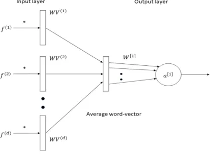
The problem we are trying to solve can be formulated as follows: Given a set of m documents with n features, the documents would be represented by matrix X ∈ Rmxn. We want to find the coefficients that predict the output Y from the documents X and we want to build a model where the coefficients (θ(i)) are a sum of the weights learnt through logistic regression and a function of its wordi

representation (v(i)), i.e.,

θ(i) =θ_lr(i)+θ(_wvi) (3.3) These new weightsθwv(i) would act as a regularization constraint so that simi-lar word representations would have simisimi-lar coefficients, which satisfies a con-tinuity condition:

|f(v(1))−f(v(2)))| ≤ sim(v(1), v(2)) (3.4) where,simdictates the similarity between wordsv(1)andv(2)andf(v(1)), f(v(2)) are coefficients of their respective words as per (3.3)

Since words used in similar context will have similar word-vectors and by making the regression co-efficient of a word to be a function of its word-vector representation, we can regularize the regression coefficients of two similar words to have similar values. So, if one word occurs more frequently and has higher regression co-efficient, the other word even if it is very rare would be con-sidered an important feature and would have a higher regression co-efficient. This would improve the classification performance in cases where these rare words occur more frequently in the test set.

Fig. 1 is a network diagram showing how the coefficients (θi) would be obtained

(21)

Figure 3.3: Network diagram to learnθ(i) from wordi representation f(v(i))

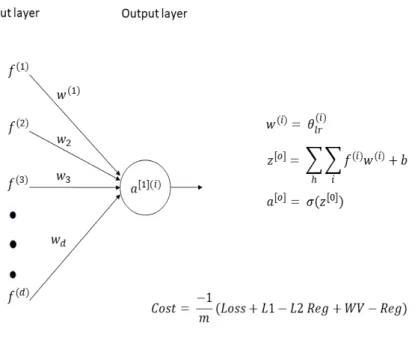
We initially explore learningθ(wvi) through regression:

Learning θ(wvi) through Regression: We determine if we can learn the

coeffi-cientsθwv(i) from the word representation of the features using a linear regressor,

i.e.,

θ(_wvi) =w1v (i) 1 +w2v

(i)

2 +...+wdv

(i)

d = D

X

d=1

w_d(i)v_d(i) _(3.5) where, w= (w1, w2, ..., wd) are the parameters of the regression function.

v = (v1, v2, ..., vd) are d-dimensional word-representations of wordi

These new weights which have been regularized through word-vectors will act as additional features to the free weights learnt through the vanilla logistic regression model. Thus the probability that class variable yj = 1, j = 1,2, ...m

can be modelled as follows:

P(yj = 1|xj;θ, w) = h(θ|w)(xj) =

1

1 +e−θTx(j) (3.6)

where, θ(i)=θlr(i)+θ

(i)

wv are the parameters of the function for feature (i) Within the class of linear functions, our task shall be to find the best parame-tersw that minimize the error function such that,

(22)

Cost(h(θ|w)(x), y) =

(

−log(h(θ|w)(x)), if y=1

−log(1−h(θ|w)(x)),if y=0

(3.7)

CNN compared with the modified model. We now compare the CNN

net-work to the modified word-vector model, where the feature coefficients are a lin-ear sum of the logistic regression weights and the weights constrained through the word vector representation. Without the vanilla logistic regression weights, the model would be same as the previous 1D CNN network. For this network, we would have to incorporate these vanilla weights to the output of the sum pooling layer before applying the sigmoid/softmax function. For this we would need a different kind of pooling layer that would sum both the pair of weights, i.e, the free vanilla weights and the word-vector weights.

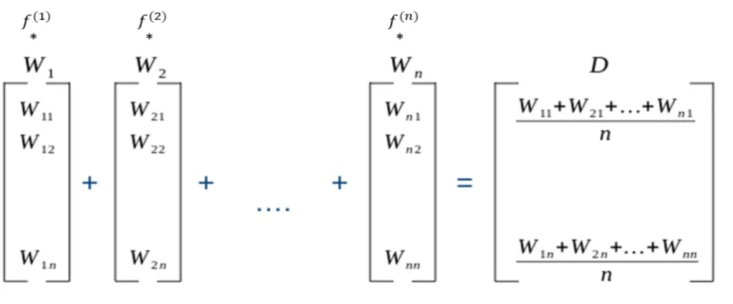
3.3 M3: Document embedding by averaging

word-vectors

We initially tried a basic scenario where documents are represented by a fixed length vector which can then be used for classification even though each doc-ument can be of a different length.

One of the common techniques to generate new embeddings to documents is by using an existing pre-trained word embeddings by averaging the word vectors to create a single fixed size embedding vector.

Figure 3.4: Average word-vectors

3.3.1 Steps to compute fixed embedding vector

(23)

Google or retrained on the training data to obtain domain specific word vectors.

• _{Then we iterate over the entire corpus and generate a mean vector for each}

document.

Once we obtain the mean vector for all the documents, we train a vanilla logistic regression model using the thus generated fixed embedding feature matrix.

Figure 3.5: Average word-vectors model

3.4 M4: Vanilla logistic regression with word-vector

regularization

Our proposed method trained a model using coefficients trained from both the vanilla logistic regression model and word-vectors. In this model, instead of generating the feature weights using the word-vectors, we use the word-vectors as a regularizer that is added to the cost function. This regularizer would add a higher penalty to similar words having large differences in their corresponding feature weights. This kind of regularization should technically enforce similar words to have similar weights.

Thus, similar to logistic regression the probability the class variable yj =

1, j = 1,2, ...m_{can be modelled as follows:} P(yj = 1|xj;θ) = hθ(xj) =

1

1 +e−θTx(j) (3.8)

Using the principle of maximum likelihood estimate, we find the parameters that maximize the likelihood P(X |y). Hence the log-likelihood is given as,

(24)

L(θ) =

m

X

i=1

yilog(hθ(xi)) + (1−yi)log(1−hθ(xi)) (3.9)

Maximizing the log-likelihood is similar to minimizing -L(θ) over all data points. The cost function for the logistic regression model comes out to be,

J(θ) = −1

mL(θ) (3.10)

Adding L1, L2 and word-vector regularization to this we get: J(θ) = −1

mL(θ) + λ1

m|θ|+ λ2

m|θ|

2

+λ3

m(W V Reg) (3.11) where λ1, λ2, λ3 and l1, l2 and word-vector regularization constraints.

Given a dataset of n features, we compute the word-vector regularization as follows:

• Compute the cosine similarity between all feature’s words-vectors. This will give us a (n x n) dimensional similarity matrix

• _{Compute the difference between the corresponding feature weights}θ_{. This} will also give us an(nxn)dimensional matrix that contains the difference between a feature’s weight to all other weights

• _{Perform a matrix multiplication between the similarity matrix and the}

matrix having the difference between the coefficients

• _{The final result will act as a word-vector regularizer which can be added}

to the overall cost function regularized by a regularization parameter λ3

Why would it work? _{Let’s say there are two words ”Russia” and ”Soviet”}

having similar word-vectors due to their reference in similar context. However the word ”Russia” is present in the text more often than ”Soviet” and has higher feature weight. Due to their high similarity and larger difference in weights, the word-vector model will add a higher penalty to the cost function until their corresponding weights are close to each other.

Now the claim is that the cost function would be minimized if the word-vector penalty is minimum. Now let’s think about a few cases:

• Case 1: _{If two features} xi,xj are completely dissimilar, their cosine

simi-larity is 0, and they don’t contribute to the cost function

• Case 2: If two features are completely alike, their cosine similarity is 1.

Now we have two subcases:

– Subcase 1: Both features have similar weights, thus the difference

between their weights is 0. This would also not contribute to the cost function.

(25)

Figure 3.6: Logistic Regression with Word-vector regularization

– Subcase 2: _{Both features have very different weights, thus the}

differ-ence between their weights would be large. This would increase the overall cost function. This is precisely the examples we are looking for: similar features having very different weights. So the algorithm forces them to have the same weights.

3.4.1 Challenges faced

The major challenge faced while running this model is the amount of time it took to generate the weight differences matrix and computing its dot product with the similarity matrix. Since the model was trained using mini-batch gra-dient descent, we had to compute the word-vector regularization cost at the end of every mini-batch in order to update the weights.

So for a medium sized dataset with 10,000 features, 100,000 records and a decent batch size of 10% of training data, one would have to compute these matrices and get their dot product at least 10 times. And that would train the model for just a single epoch. For training a good enough model with a decent learning rate, one would need to train the model for at least 400-500 epochs. All of this only if we are training a binary classifier. If we are training a multi-class or multi-label multi-classifier with ∼2000 different classes, then it would take an exponential amount of time. This puts a huge constraint on the amount of time and resources needed to train the model. For training an even larger dataset with ∼100,000 features, it would be even more difficult as training a single epoch itself might take a few hours.

(26)

3.4.2 Workarounds

In order to remediate this, we limit the features for which we want to increase the weights. Since our objective through this project was to make rare features have higher weights, we can pick the top k rarest features and look at their similarities with the rest of the features. This would reduce the similarity matrix size from (n x n) to (n x k). We can choose the top rare features based on their IDF (Inverse Document Frequency) score.

Inverse docment frequency or IDF is a numerical statistic used in informa-tion retrieval to reflect how rare a term is. It is known that certain terms, such as ”is”, ”of”, and ”that” may appear a lot of times but have little importance. IDF helps in weighing down the frequent terms and finding the rare ones by computing the following:

IDF =loge(

T otalnumberof documents

N umberof documentswithtermtinit) (3.12) Once we decide on the total number of top rare features, the rest of the steps remain same as before with the only change being that we compute the cosine similarity and difference in coefficients matrix for only these top features and add the resulting value as the word-vector regularization cost.

(27)

Chapter 4 Experiments

We compare our model to the vanilla logistic regression algorithm by imple-menting both using the TensorFlow library. Both the models can perform multi-class and multi-label classification. For multi-class, we use the softmax function to assign probabilities to each class which add up to 1. We use the sigmoid function for multi-label classification to train an independent logistic regression model for each class and accept all labels greater than a certain threshold as predictions.

We tune our model using learning rate and regularization parameter as hyper-parameters and train with different number of epochs till the loss con-verges. For multi-label problems, we also use prediction threshold as one of the hyper-parameters to list labels with probabilities greater than the threshold value.

4.1 Training stopping criteria and batches

We initially trained the model for a predetermined number of iterations and noted the overall cost at the end of each iteration. If we notice the cost to be still decreasing after the predetermined set of iterations, we continue training the model for more epochs. We do this until the cost does not reduce any further thereby giving us the lowest possible minima.

Also in order to find the minima in a reasonable amount of time, we trained the model on mini-batches and updated the weights after computing the cost at the end of each mini-batch cycle. (commonly known as mini-batch gradi-ent descgradi-ent) Some of the datasets we worked with had imbalanced data where some of the classes were not represented equally. For eg., we have seen that the Reality-TV(68) and News(12) classes have very few positive samples as com-pared to the total number of samples ( 35,000). This is an imbalanced dataset and the imbalance ratio is 500:1 and 2900:1 for the Reality-TV and News classes respectively. We can have a class imbalance problem over multi-class or multi-label problems.

In order to handle this data imbalance, we tried resampling the data for these rare classes so that our predictive model would have more balanced data to work with. To balance the data, we over-sampled the rare class by adding copies of instances from the under-represented class. This technique is also

(28)

known as sampling with replacement. We thus made sure that while training a model on the rare class, each mini-batch had 50% positive samples (data belonging to that class) and 50% negative samples.

4.2 Pyramid implementation

We also trained our model through Pyramid, a Java machine learning library developed by one of Dr.Pavlu’s PhD student, Cheng Li. It has many state-of-the-art machine learning algorithms implemented which we used to compare our model performance with. More details about Pyramid can be found in the link below:

• _{https://github.com/cheng-li/pyramid}

4.3 Evaluation

To evaluate the performance of both models for multi-class problems, we use accuracy and F1 measures.

For multi-label problems, predictions for an instance is a set of labels, and therefore the prediction can be fully correct, partially-correct or fully-incorrect. Thus, to better evaluate our models we will use the following three measures:

set accuracy, which is the ratio of perfectly matched instances to the total num-ber of instances;instance-F1, which evaluates the performance of partially cor-rect predictions averaged over instances; label-F1, which evaluates the perfor-mance of partially correct predictions averaged over labels.

For a dataset with ground truth labels y(n) and predictions yˆ(n), and n in-stances where n = 1,2,...,N, these three measures are defined as:

set accuracy= 1 N

N

X

n=1

I(y(n) = ˆy(n)) (4.1)

instance-F1 = 1 N

N

X

n=1

2PL

l=1y (n)

l yˆ

(n)

l

PL

l=1y (n)

l +

PL

l=1yˆ (n)

l

label-F1= 1 N

N

X

n=1

2PN

n=1y (n)

l yˆ

(n)

l

PN

n=1y (n)

l +

PN

n=1yˆ (n)

l

(4.2) where for each instance n, yl(n) = 1 if label l is a given label in ground truth;

ˆ

y_l(n) _{= 1 if label}l _{is a predicted label.}

4.4 IMDb dataset

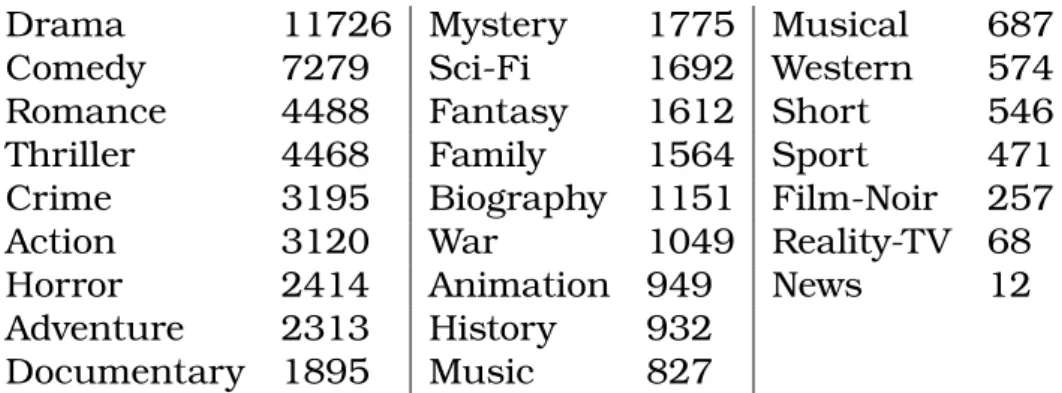
The IMDb dataset is created by Meka with movie plot text summaries labelled with genres sourced from the Internet Movie Database Interface. It is a collec-tion of 35,000 documents particollec-tioned across 25 different genres. The task is to assign multiple genres to a movie description.

(29)

Drama 11726 Mystery 1775 Musical 687

Comedy 7279 Sci-Fi 1692 Western 574

Romance 4488 Fantasy 1612 Short 546

Thriller 4468 Family 1564 Sport 471

Crime 3195 Biography 1151 Film-Noir 257

Action 3120 War 1049 Reality-TV 68

Horror 2414 Animation 949 News 12

Adventure 2313 History 932 Documentary 1895 Music 827

Table 4.1: The 24 topic categories for the IMDb dataset with the number of examples assigned to them.

Below is a list of the 25 different genres with individual genre counts. We evaluate how the model performed on the IMDb dataset by comparing its performance with the vanilla logistic regression model. We compare both the overall model performance as well as the individual label performance.

4.4.1 Overall Model Performance

We initially look at how the overall model performed. Since each document in the IMDb dataset can belong to multiple genres, we’re trying to solve a multi-label classification problem. For multi-multi-label classification, as discussed previ-ously in equation 4.1, we will use Set-Accuracy and Instance-F1 measures to evaluate the model. Along with evaluating the model on the vanilla logistic re-gression and our word-vector model, we also evaluate the model on pyramid’s version of logistic regression. Below is how each of the model’s performed.

Looking at the results, we can see that our model has outperformed both the pyramid and vanilla logistic regression models on both Set-Accuracy and Instance-F1.

IMDb Set Accuracy Instance F1

M3: Doc-Avg wv embedding 7.3 45.2

M1: Initial WV model 6.1 45.69

M4: Regression + WV Penalty _17.19 _56.32

Pyramid LR 19.66 56.14

Tensorflow LR 18.21 57.87

M2 : Sum-weights WV Model _20.30 _58.52

(30)

4.4.2 Individual Label Performance

Below is a table showing the individual label performance between both mod-els which has been sorted in descending order of its performance improvement.

Label Tensorflow LR Label F1

Our Model Label F1

Percentage Improvement

News 0.00 50.00 50.00

Musical 33.54 43.78 10.24

Animation 44.66 50.23 5.57

Sport 61.65 67.13 5.47

Film Noir 25.31 30.23 4.91

War 58.64 62.92 4.27

Sci-Fi 68.83 72.73 3.89

Adventure 52.44 56.14 3.7

Music 54.08 56.98 2.9

Crime 60.24 62.72 2.48

Documentary 71.05 73.36 2.31

Short 56.06 58.23 2.17

Family 51.07 53.21 2.14

Comedy 62.87 64/67 1.8

Romance 51.17 52.5 1.33

Fantasy 41.96 43.05 1.09

Mystery 47.91 48.61 0.7

Horror 64.23 64.8 0.57

History 38.01 38.33 0.32

Western 77.21 77.38 0.17

Biography 39.36 38.17 -1.19

Drama 73.45 72.24 -1.21

Thriller 54.86 51.81 -3.05

Action 18.18 11.54 -6.64

(31)

Deeper analysis of label - News:

From the above table we can see that the vanilla logistic regression model performed very badly on the News dataset as compared to our new model. Upon further investigating the dataset, we found that this particular label had only 12 records in total, out of which 9 were train and 3 were test.

Below was the train and test performance of both the models on the News label.

F1 TN FP FN TP

train _0.00 ₂₂₄₁₂ ₀ ₉ ₀

test 0.00 3114 1 3 0

Table 4.4: Vanilla logistic regression train-test performance on News Label.

F1 TN FP FN TP

train 100.00 22412 0 0 9

test _50.00 ₃₁₁₅ ₀ ₂ ₁

Table 4.5: Word-vector model train-test performance on News Label. Upon just looking at the train performance of both models, we can see that the vanilla logistic regression model has predicted 0 true positives, while our model predicted all 9 true positives correctly and has an F1 score of 100%. Predictably looking at the train performance, the vanilla model did not per-form well on the test set as compared to the word-vector model. This example proves that the word-vector model can perform well even with very few training records.

Deeper analysis of label - Musical:

Let’s look at another labelMusical which has more positive examples than the previous case. This particular label had 687 train and 109 test records and below is the model performance on both the train and test splits for both the vanilla logistic regression and the word-vector models.

F1 TN FP FN TP

train 82.88 21730 4 198 489

test 33.54 2984 25 82 27

Table 4.6: Vanilla logistic regression train-test performance onMusical Label. From the above tables, we can see that the word-vector model was able to predict correctly more true positives and lesser false negatives on the train dataset. This performance carried over to the test set as well. Also looking at the train and test F1 scores of both models, we can see that there is a bigger difference in train-test scores of the logistic regression model as compared to the word-vector one. We noticed this trend in general where the word-vector

(32)

F1 TN FP FN TP

train 85.07 21724 10 171 516

test 43.79 2986 23 72 37

Table 4.7: Word-vector model train-test performance on Musical Label. model is less likely to overfit.

Deeper analysis of label - Action:

Let’s look at a label from the bottom end of the table - Action. This label had 257 train and 44 test documents and below is how the model performed.

F1 TN FP FN TP

train _86.53 ₂₂₁₆₄ ₀ ₆₁ ₁₉₆

test 18.18 3068 6 39 5

Table 4.8: Vanilla logistic regression train-test performance on ActionLabel.

F1 TN FP FN TP

train 84.49 22164 0 69 188

test _11.54 ₃₀₆₉ ₅ ₄₁ ₃

Table 4.9: Word-vector model train-test performance on ActionLabel. Looking at the performance we can see that the word-vector model predicted more false negatives as compared to the vanilla model. However looking at the test performance, we can see that our model predicted only 2 fewer true positives as compared to the vanilla model. This might’ve been caused due to fewer training samples or it was a difficult label to train.

(33)

4.5 Guardian dataset

The Guardian is a National British daily newspaper, known until 1959 as the Manchester Guardian. Its online edition was the fifth most widely read in the world as of October 2014, with over 42 million readers. This dataset contains articles on various topics like World news, UK news, Culture, Politics, Media, Business, Society etc.

All the data had been manually scrapped from the Guardian website with each file containing a document and its associated tags. The dataset in use contains 20 different classes and the task is to assign multiple tags to each news article.

Below is a list of the 20 different genres.

Blogging LGBT rights

Christianity Mental health

Comedy Poetry

Computing Premier League

Counter-terrorism policy Public finance

Drugs Public sector cuts

Financial crisis Research Global enonomy Restaurants Health policy Retail industry

Inequality Tax and spending

Table 4.10: The 20 topic categories for the Guardian dataset with the number of examples assigned to them.

4.5.1 Overall Model Performance

Like the IMDb dataset, each document of the Guardian dataset can belong to multiple tags. So this will also be a multi-label classification problem, and we will be using Set-Accuracy and Instance-F1 measures to evaluate the model. Along with evaluating the model on the vanilla logistic regression and our word-vector model, we also evaluate the model on pyramid’s version of logistic regres-sion. Below is how each of the model’s performed.

Guardian Set Accuracy Instance F1

M3: Doc-Avg wv embedding 43.65 60.61

M1: Initial WV model _42.36 _59.65

Pyramid LR 59.3 65.13

(34)

4.5.2 Individual Label Performance

Below is a table showing the individual label performance between both models which has been sorted in descending order of its performance improvement. For this dataset, we did not get any labels that performed badly on the word-vector model as compared to the logistic regression model.

Our Model Label F1

Drugs 80.5 88.75 8.25

Mental health 69.23 76.8 7.57

Global economy 56.34 62.69 6.35

LGBT 76.84 82.9 6.06

Blogging 77.3 82.72 5.42

Public finance 48.24 53.33 5.09

Premier League 90 95.03 5.03

Research 60.97 65.84 4.87

Retail 79.78 84.62 4.84

Inequality 50.3 55.12 4.82

Tax and Spending 50.73 54.35 3.62

Counter-terrorism 88.88 91.5 2.62

Restraunts 88.72 91.05 2.33

Health policy 68.08 70.27 2.19

Poetry 89.17 91.14 1.97

Financial Crisis 49.43 50.87 1.44

Computing 69.82 71.01 1.19

Public sector cuts 56.83 57.79 0.96

Comedy 77.1 77.65 0.55

Christianity 75 75.47 0.47

Table 4.12: Guardian Model Performance at a Label level.

Deeper analysis of label - Drugs:

Let’s look at the model with the biggest F1 gainsDrugs. This label had 625 positive samples of news articles labelled Drugs. Out of these 545 belonged to the trainset and 80 belonged to the testset. Below was the train and test performance of both the models on theDrugs label.

F1 TN FP FN TP

train 92.46 10632 19 60 485

test 80.50 1463 15 16 64

Table 4.13: Vanilla logistic regression train-test performance on Drugs Label. From the above metrics, we can see that the word-vector model got more true positives and fewer false negatives, false positives as compared to the vanilla logistic regression model leading to higher F1 score. This performance

(35)

F1 TN FP FN TP

train 94.91 10639 12 42 503

test 88.75 1469 9 9 71

Table 4.14: Word-vector model train-test performance on Drugs Label. improvement can be observed on both the train and test datasets.

Deeper analysis of label - Global Economy:

Looking at another labelGlobal economy, which has 605 train and 72 test samples and juxtaposing their model performances. Comparing just the train performance of both models, we can see that the vanilla model got almost 20 true positives right as compared to the word-vector model. However, when you look at their corresponding test performances, we can that the word-vector model got 2 extra true positives right as compared to the vanilla version. This shows that the vanilla model was clearly overfitting on the trainset and per-formed badly on the testset, while the word-vector model is not so much prone to overfitting. Hence we see a much higher test F1 score for the word-vector model as compared to the vanilla model.

F1 TN FP FN TP

train 87.36 10541 50 97 508

test 56.33 1456 30 32 40

Table 4.15: Vanilla logistic regression train-test performance on Global

econ-omyLabel.

F1 TN FP FN TP

train _88.31 ₁₀₅₇₅ ₁₆ ₁₁₄ ₄₉₁

test 62.69 1466 20 30 42

Table 4.16: Word-vector model train-test performance onGlobal economy La-bel.

Deeper analysis of label - Christianity:

Analyzing a label from the bottom of the table we see that the logistic regres-sion model already had a very high train F1 score and the word-vector model was not able to improve much on this.

Looking at the results, we can see that our model has outperformed both the pyramid and vanilla logistic regression models on both Set-Accuracy and Instance-F1.

(36)

F1 TN FP FN TP

train 91.75 10461 37 75 623

test 75.00 1453 13 29 63

Table 4.17: Vanilla logistic regression train-test performance on Christianity Label.

F1 TN FP FN TP

train 93.39 10478 20 69 629

test _75.47 ₁₄₅₉ ₇ ₃₂ ₆₀

Table 4.18: Word-vector model train-test performance on Christianity Label.

4.6 Medical dataset

The medical dataset contains radiology patient data from the MGH hospital. It consits of about 2670 classes which are diagnosis codes used to bill the in-surance company. It is a collection of 650,000 instances with 11,000 features. This is a multi-label classification problem and the task is to assign multiple diagnosis codes to the patient data.

We evaluate how the model performed on the Medical dataset by comparing its performance with the vanilla logistic regression model. We compare both the overall model performance as well as the individual label performance.

4.6.1 Overall Model Performance

Looking at the overall results, we can see that there is a big difference in perfor-mance of both models. This may have been because the model wasn’t trained enough and it had a strong label dependency which affected multi-label eval-uation.

Medical Set Accuracy Instance F1

Table 4.19: Set-Accuracy and Instance-F1 Results for Medical dataset.

4.6.2 Individual Label Performance

Below is a table showing the individual label performance between both models which has been sorted in descending order of its performance improvement.

(37)

Our Model Label F1

Abnormal findings 19.59 82.85 63.26

Osteoarthritis knee 17.20 80.10 62.89

Soft tissue disorders 10.91 69.57 58.66

Primary osteoarthritis 17.14 73.59 56.45

Pleural effusion 23.61 78.1 54.49

Cough 31.43 85.86 54.43

Pneumothorax 42.18 75.56 33.38

Dyspnea 23.77 49.01 25.24

Malignant neoplasm

of breast 95.86 99.87 3.98

Table 4.20: Medical dataset model performance at a label level.

4.7 20 Newsgroups dataset

The 20 Newsgroups dataset is a collection of approximately 20,000 newsgroup documents, partitioned (nearly) evenly across 20 different newsgroups. It has become a popular data set for experiments in text applications of machine learning techniques, such as text classification and text clustering.

The data is organized into 20 different newsgroups, each corresponding to a different topic. Some of the newsgroups are very closely related to each other (e.g. comp.sys.ibm.pc.hardware / comp.sys.mac.hardware), while others are highly unrelated (e.g misc.forsale / soc.religion.christian). Except for a small fraction of the articles, each document belongs to exactly one newsgroup. The task is to learn which newsgroup an article was posted to. Below is a list of 20 newsgroup partitioned according to their subject matter.

comp.graphics

comp.os.ms-windows.misc rec.autos sci.crypt comp.sys.ibm.pc.hardware rec.motorcycles sci.electronics comp.sys.mac.hardware rec.sport.baseball sci.med

comp.windows.x rec.sport.hockey sci.space

talk.politics.misc talk.religion.misc misc.forsale talk.politics.guns alt.atheism

talk.politics.mideast soc.religion.christian Table 4.21: Newsgroups used in newsgroups data

4.7.1 Overall Model Performance

Each document in the belongs to one of the 20 classes. So unlike the IMDb and Guardian dataset where we were solving multi-label classification, for this dataset we are solving a multi-class classification problem. So we do not have metrics like Set-Accuracy or Instance-F1 to compute the model performance.

(38)

We instead will only use the F1 score over the entire dataset. Below is how each of the models performed.

20Newsgroup F1 Score

M3: Doc-Avg wv embedding _45.80

M1: Initial WV model 49.5

M4: Regression + WV Penalty 55.48

Pyramid LR 55.64

Tensorflow LR 55.75

M2 : Sum-weights WV Model 58.80

Table 4.22: Overall F1 Results for 20 Newsgroup dataset.

Looking at the results, we can see that our model has outperformed the pyramid and vanilla logistic regression models.

We evaluate how the model performed on the 20 Newsgroup dataset by com-paring its performance with the vanilla logistic regression model. We compare both the overall model performance as well as the individual label performance.

4.7.2 Individual Label Performance

Below is a table showing the individual label performance between both mod-els which has been sorted in descending order of its performance improvement.

Label Tensorflow LR

Label F1

Our Model Label F1

comp.sys.ibm.pc.hardware 48.98 56.68 7.7

soc.religion.christian 58.24 64.09 5.85

talk.politics.misc 46.45 51.9 5.45

comp.os.ms-windows.misc 55.17 60.3 5.13

comp.graphics 51.81 56 4.19

comp.windows.x 67 71 4

sci.electronics 51.04 55.03 3.99

comp.sys.mac.hardware 54.8 57.83 3.03

alt.atheism 44.44 46.27 1.83

sci.space 66.67 67.82 1.15

rec.sport.baseball 72.63 73.3 0.67

talk.politics.guns 55.17 55.81 0.64

talk.religion.misc 37.21 37.68 0.47

sci.med 68.13 68.06 -0.07

sci.crypt 75.36 75.12 -0.24

rec.autos 53.95 53.5 -0.45

talk.politics.mideast 76.65 76.02 -0.63

misc.forsale 67.84 66.09 -1.75

rec.motorcycles 60.47 58.7 -1.77

rec.sport.hockey 86.17 84.21 -1.96

(39)

Deeper analysis of label - comp.sys.ibm.pc.hardware:

Let’s look at the model with the biggest F1 gainscomp.sys.ibm.pc.hardware. This label had 797 positive samples. Out of these 696 belonged to the trainset and 101 belonged to the testset. Below was the train and test performance of both the models on the comp.sys.ibm.pc.hardwarelabel.

F1 TN FP FN TP

train 95.81 12435 1 55 641

test 48.98 1782 47 53 48

Table 4.24: Vanilla logistic regression train-test performance on the

comp.sys.ibm.pc.hardware_label.

F1 TN FP FN TP

train 98.54 12436 0 20 676

test 56.68 1796 33 48 53

Table 4.25: Word-vector model train-test performance on the

comp.sys.ibm.pc.hardwarelabel.

We can see that the word-vector model got much higher true positives and fewer false negatives as compared to the vanilla model for the trainset. And this performance is also reflected in the testset.

Deeper analysis of label - talk.politics.misc:

Analyzing the performance of another label talk.politics.misc which has 636 total samples out of which 548 are train and 88 are test. Below is how both the models performed on thetalk.politics.misc label.

F1 TN FP FN TP

train _96.03 ₁₂₅₈₂ ₂ ₄₀ ₅₀₈

test 46.45 1811 31 52 36

Table 4.26: Vanilla logistic regression train-test performance on the

talk.politics.misc label.

From the above performance results, we can see that the vanilla logistic regression model already had a very high train F1 score. In-spite of that, the word-vector model managed to further improve it by predicting more true pos-itives correctly.

(40)

F1 TN FP FN TP

train 97.95 12584 0 22 526

test 51.9 1813 29 47 41

Table 4.27: Word-vector model train-test performance on the

talk.politics.misc label.

4.8 Additional tests

We also ran a validation experiment with artificially modified dataset on the 20 newsgroup dataset to mimic sparse representation: To do this we found the most similar words in the train set with cosine similarity greater than 0.3 and make the feature values of all but one of the words equal to zero. We then com-pared the performance of our model with logistic regression before and after zeroing feature values of similar words. The below results show that our model was able to get a good test accuracy after the imposed sparsity.

Logistic regression M2 : Sum-weights WV Model Before zeroing features 82.6 84.01

After zeroing features 75.67 83.54

(41)

Chapter 5 Analysis

Each feature of the word-vector model obtains its co-efficients from two sepa-rate sources:

• _{the first set of weights are trained in a similar fashion to the vanilla logistic}

regression model

• the second set of weights are learnt by enforcing a word-vector regular-ization

We train the model as follows:

We initially keep word-vector weights constant at zero. We then find the best model performance by training only the vanilla logistic regression model through extensive hyper-parameter tuning (l1/l2 regularization).

Once the vanilla feature weights have been learnt, we then start learning the word-vectors weights by increasing the l1/l2 regularization on the vanilla fea-ture weights. This regularization would force the model to reduce the strength of the vanilla weights and move them to the unregularized word-vector weights. As the l1/l2 regularization strength per feature starts increasing, more and more weight from the vanilla model starts to shift onto the word-vector feature weights. The word-vector weights are constrained by a word-vector function. So when the word-vector model weights are substantial enough, then due to the word-vector similarity property, we are able to see the weights of the rare similar words also to start having a higher weight. This boosting of the rare word-weights would help improving the performance of the model.

However it is also possible that some labels better perform using the vanilla weights rather than the word-vector weights. In such a case, applying high regularization on the vanilla weights to boost the word-vector weights would be counterproductive. Thus, we need to perform extensive hyper-parameter tuning to find the right set of vanilla and word-vector weights that would work on all kinds of labels.

We performed several experiments to find the right set of hyper-parameters. Through these experiments we noticed that if the l1 penalty on the vanilla weights was too low, then the word-vector weights wouldn’t increase much at all. They would remain almost close to zero. As we applied more and more l1 penalty, the model was forced to learn through the word-vector weights.

(42)

Below is a graph showing various test results comparing l1 constraint per feature versus word-vector weights. We can see that the word-vector weights were increasing with higher L1 up to a certain point. After a certain threshold, the word-vector weights were almost non-increasing.

We also compared the model performance vs L1 strength. We can clearly see that the model performance increases initially with increasing L1 regular-ization and after a certain threshold, we see the model performance start to go down.

Figure 5.1: Graph comparing word-vector weights with increasing L1 regular-ization

Upon comparing both models, we noticed that the performance of the word-vector models improved due to the additional word-word-vector weights.

To verify this, we took the top features for each model and printed the fol-lowing:

• _{top similar words for each feature calculated based on the cosine}

similar-ity of the word-vectors

• cosine similarity of the similar word

• _{feature weight of the similar word} • _{idf score of the similar word}

The idf scores were computed to measure the rarity of the words. We noticed that the rare features which were similar to the important features now had similar weights. The below section shows such examples:

Northeastern University