RESEARCH ARTICLE
Efficiency of different measures
for defining the applicability domain
of classification models
Waldemar Klingspohn
1, Miriam Mathea
1, Antonius ter Laak
2, Nikolaus Heinrich
2and Knut Baumann
1*Abstract
The goal of defining an applicability domain for a predictive classification model is to identify the region in chemical space where the model’s predictions are reliable. The boundary of the applicability domain is defined with the help of a measure that shall reflect the reliability of an individual prediction. Here, the available measures are differenti‑ ated into those that flag unusual objects and which are independent of the original classifier and those that use information of the trained classifier. The former set of techniques is referred to as novelty detection while the latter is designated as confidence estimation. A review of the available confidence estimators shows that most of these measures estimate the probability of class membership of the predicted objects which is inversely related to the error probability. Thus, class probability estimates are natural candidates for defining the applicability domain but were not comprehensively included in previous benchmark studies. The focus of the present study is to find the best measure for defining the applicability domain for a given binary classification technique and to determine the performance of novelty detection versus confidence estimation. Six different binary classification techniques in combination with ten data sets were studied to benchmark the various measures. The area under the receiver operating characteristic curve (AUC ROC) was employed as main benchmark criterion. It is shown that class probability estimates constantly perform best to differentiate between reliable and unreliable predictions. Previously proposed alternatives to class probability estimates do not perform better than the latter and are inferior in most cases. Interestingly, the impact of defining an applicability domain depends on the observed area under the receiver operator characteristic curve. That means that it depends on the level of difficulty of the classification problem (expressed as AUC ROC) and will be largest for intermediately difficult problems (range AUC ROC 0.7–0.9). In the ranking of classifiers, classification random forests performed best on average. Hence, classification random forests in combination with the respective class probability estimate are a good starting point for predictive binary chemoinformatic classifiers with applicability domain. Keywords: Applicability domain, Applicability domain measures, Reject option, Novelty detection, Confidence estimation, Class probability estimation
© The Author(s) 2017. This article is distributed under the terms of the Creative Commons Attribution 4.0 International License (http://creativecommons.org/licenses/by/4.0/), which permits unrestricted use, distribution, and reproduction in any medium, provided you give appropriate credit to the original author(s) and the source, provide a link to the Creative Commons license, and indicate if changes were made. The Creative Commons Public Domain Dedication waiver (http://creativecommons.org/ publicdomain/zero/1.0/) applies to the data made available in this article, unless otherwise stated.
Background
Classification rules are often used in chemoinformatics to predict categorical properties such as bioactivity, toxicity or metabolic stability of drug candidates. The classifica-tion rule is derived from n training set compounds where
each chemical compound is represented by p explana-tory variables (molecular descriptors) and a class label or property value [1, 2]. In the productive phase of the classifier, new objects (future objects) are predicted using only the information of their molecular descriptors [3, 4]. For decision making, e.g. for prioritizing the order of synthesis of candidate molecules, an important piece of information is the uncertainty associated with the predic-tion of a particular molecule. The predicpredic-tion error, esti-mated with an independent test set, provides important
Open Access
*Correspondence: k.baumann@tu‑braunschweig.de 1 Institute of Medicinal and Pharmaceutical Chemistry, University of Technology Braunschweig, Beethovenstrasse 55, 38106 Brunswick, Germany
information on the average performance of the employed classifier. However, it cannot provide information about the probability of misclassification for a particular mole-cule. There are two situations where the individual prob-ability of misclassification may differ significantly from the average probability of misclassification (i.e. the pre-diction error). First, a future object may be dissimilar to the training objects in terms of its molecular descriptors. It is reasonable to expect a larger probability of misclas-sification for those molecules that are located in sparsely populated regions of the training data set. Second, a future object may be located close to the decision bound-ary of the classifier. In most real-world data sets class overlap is strongest in that region. This may be due to label noise (i.e. the feature that determines the class label can only be determined up to a certain precision) or due to imperfect molecular descriptors that cannot differenti-ate between subtle features of the classes. In any case, the user may wish to be informed about uncertain predic-tions. This is commonly done by defining an applicability domain (AD) in chemoinformatics. The latter is defined as the “response and chemical structure space in which the model makes predictions with a given reliability” [5]. Predictions for molecules located outside the AD are considered to be unreliable. An AD is one of the pillars of a validated model according to the OECD principles for quantitative structure–activity relationship (QSAR) models [6].
While it is pretty straightforward to define the ments for an ideal AD, it is less clear how these require-ments can be achieved. How can the response and chemical structure space be narrowed down so that only reliable predictions remain? In the first case mentioned above various distance measures have been employed as to characterize how well the future object is embedded in the training set [7–10]. If the future object is too remote from the training data set, its prediction is rejected. Remote objects typically contain novel concepts not rep-resented in the training data set which increases the error probability. Identifying remote objects is often termed novelty detection, anomaly detection or outlier detec-tion in machine learning [8, 11–14]. In the following, the term novelty detection is used. In novelty detection the training data set is used to define a region with known objects and any object that does not belong to this region is flagged as novel. Since only the class of normal objects is defined (i.e. the training set) while the class of novel objects is ill-defined, this is a so-called one-class classi-fication problem and any one-class classifier can be used for novelty detection. It is important to note that the one-class one-classifier used for novelty detection does neither use the class label information of the objects in the training data set nor information of the underlying classifier that
is used to predict the object’s class label. Novelty detec-tion solely uses the explanatory variables to set up a sec-ond classifier to determine whether or not a future object is close enough to the known objects.
Remoteness to the training data certainly determines the reliability of a prediction. However, an even stronger predictor for the expected probability of misclassification should be an object’s distance to the decision boundary of the classifier. A small distance to the decision bound-ary was the second case mentioned above that may yield an error probability above average. Characterizing the probability of misclassification of an individual object has been termed confidence estimation [15, 16]. As opposed to novelty detection, confidence estimation uses informa-tion of the underlying classifier. Most confidence meas-ures are built-in measmeas-ures of the employed classifier that characterize, one way or the other, the distance of the future object to the decision boundary. This distance is then converted to a degree of class membership. These values can be strict probabilities such as the posterior probabilities in linear discriminant analysis or they can be uncalibrated scores. In this case, the only property that holds is that a higher score indicates a higher prob-ability of class membership [17, 18]. There are tech-niques to convert uncalibrated scores into estimated class probabilities [19–21]. If calibrated properly, the class membership probability is related to the probability of misclassification for that object. Confidence estimators can also be derived from ensemble predictions by using the classifier stability to estimate a class membership score [22]. Ensemble members of a stable classifier always predict the same class for a particular object. An instable classifier varies in its predictions. The fraction of votes for one class can be used as a class membership score.
confidence measures of recent powerful classification methods were not yet benchmarked. The goal of this study is twofold: First, various AD measures are bench-marked in order to identify measures that best charac-terize the probability of misclassification for individual predictions. Since there is an interplay between classi-fication method and AD measure and since not all AD measures can be computed for every classifier, the opti-mal match between classifier and AD measure is sought. Second, a comparison of novelty detection against confi-dence estimation for defining the AD is provided. As an aside, the results of this benchmark are also of interest for setting up conformal predictors, which are an alter-native to defining the AD of a chemoinformatic classifi-cation model [24–27]. An important ingredient of each conformal predictor is a so-called nonconformity score. AD measures can be used for the latter purpose. The bet-ter the nonconformity score characbet-terizes the probability of misclassification of an individual prediction, the more efficient will be the resulting conformal predictor. That in turn means that the best AD measure will result in the most efficient conformal predictor. For more details on conformal prediction, the reader is referred to a recent monograph [28].
Random forests (RF), ensembles of feedforward neural networks (NN), support vector machines (SVM), ensem-bles of boosted classification stumps (MB), k-nearest neighbor classification (k-NN) and linear discriminant analysis (LDA) are evaluated with various AD meas-ures on ten different benchmark data sets. The selec-tion of classifiers is meant to represent a broad variety of well-established classification techniques. Deep neural networks [29] are not covered here. AD measures are computed for independent test sets, simulating future predictions, and are used to compute receiver operator characteristic (ROC) curves. The area under the ROC curve AUC ROC is the primary benchmark criterion to assess how well a particular AD measure can rank pre-dictions from most reliable to least reliable. The paper is organized as follows: In the next section, a brief overview of the employed methods is given. The focus is on the AD measures. Afterwards, the results are reported and discussed. In the following, matrices are given in bold uppercase letters (A) while vectors are represented by bold lowercase letters (a).
Methods
Classification methods, model validation and benchmarking criteria
RF, NN, SVM, MB, k-NN and LDA were run with hyper-parameter settings that perform well on average (mostly default parameters) and no hyperparameter optimization was carried out. This may lead to suboptimal models for
some data sets but the differences to the optimal models are expected to be small. Moreover, slightly suboptimal models will in general not alter the ranking of the stud-ied AD measures. Since establishing the latter is the ulti-mate goal of the study, frozen hyperparameters simplify matters here. The exact settings can be found in Addi-tional file 1. Fivefold cross-validation (CV) was used to estimate the prediction error of the classifiers. Since no hyperparameter optimization is done here and thus no model selection is necessary, there is no model selection bias [30–32]. Hence, fivefold CV represents a repetitive partitioning of the data into a training set and an inde-pendent test set, which allows estimating the prediction error and derived metrics unbiasedly for a training set size of 4/5th of the data (i.e. the employed training set size in fivefold CV). If the size of the smaller class was less than 40% of the data set size, random undersampling CV (RUS CV) [33, 34] was used to estimate the predic-tion error to account for class imbalance. Since class imbalance was not severe in most cases, the differences between plain CV and RUS CV are generally small. Addi-tional file 1 provides more details about model validation and the computation of the employed figures of merit. Three performance curves and benchmarking criteria derived thereof were used: ROC curves [35], cumulative accuracy [9, 23], and predictiveness curves [36–39]. For computing each curve, the data are first properly ranked according to the AD measure. Additional file 1 provides detailed information about the performance curves and the necessary specifics for benchmarking novelty scores with ROC curves as well as significance testing of AUC ROC with a permutation test (see also Additional file 2).
Data sets and molecular descriptors
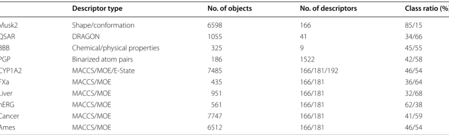
All studied datasets are publicly available. A summary of their characteristics is shown in Table 1. More detailed information can be obtained from the corresponding ref-erences. As can be seen in Table 1 the data sets vary in terms of size and class ratio. For four data sets (MUSK2 [40, 41], QSAR [42, 43], BBB [44], PGP [45]) the previ-ously published descriptors were used. For the remain-ing six data sets (FXa [46, 47], Liver [48],CYP1A2 [23, 49], hERG [50], Cancer [51], Ames [52]) the provided SMILES were used to calculate two types of molecu-lar descriptors: MACCS Keys (166 bit; the frequency of substructures is recorded) [53] and 181 MOE descriptors (those that are rotationally and translationally invari-ant). In addition to MACCS and MOE descriptors, for CYP1A2 the provided E-State descriptors were also used.
Additional file 3 (Table S13). Except for the MACCS fin-gerprints and the binarized atom pairs, all descriptors were auto-scaled, i.e. the column mean was subtracted and the mean-centred data were afterwards divided by the standard deviation of that column. Autoscaling was done prior to model building on the entire data matrix. The source of the data as well as the data are provided in the Additional files 4, 5. Those descriptors that were autoscaled prior to the analysis are provided in their autoscaled form. The remaining descriptors are provided as raw data. That means that the data are provided in the way they were used for the respective computations. In addition to the data, the indices for the fivefold CV splits are also provided. For the Ames data set the previously published partitions were used [52]. For the remaining data sets random partitions were generated.
Applicability domain measures
Sushko et al. [9, 55] introduced the term distance to model (DM) as an umbrella term for applicability domain measures. It represents a metric measure that defines the similarity between the training set objects and test set objects (in the validation phase) or future objects (in the productive phase) for a given predictive chemoinfor-matic model. It is defined to monotonically increase as the (expected) accuracy of the model decreases. While this term is well established, it is somehow misleading since most employed measures are no distances. Hence, the more general umbrella term of applicability domain measure is preferred here. In accord with Sushko et al., larger AD measures indicate a larger error probability for the respective prediction. The AD measure is the basis for defining the AD. Objects with AD values less than a predefined threshold are considered to be inside the AD. The threshold can be found in different ways. One way would be to set the threshold depending on the expected
overall accuracy for future predictions (see ‘Cumulative Accuracy’; Additional file 1) [9]. Another way would be to use the 100 − x% quantile of the training set’s AD val-ues as threshold. This would exclude the x% of the most extreme training set objects and future objects that are more extreme than the threshold [9]. A third way would be to limit the expected maximum local error rate, which is defined here as the expected error rate for a given size of the AD value. If the AD measure works efficiently, there will be a relationship between the error rate and the AD value. This relationship can be used to look up the quantile of the AD values which yields a local error rate smaller than a predefined value (see ‘Predictiveness Curves’; Additional file 1). Using a threshold on the AD value to reject predictions that are deemed too uncertain will be referred to as a reject option in accord with the classification literature [56].
DA‑index (κ, γ, δ)
This measure is based on the k-NN approach. Either the Euclidean distance (ED) or one minus Tanimoto similar-ity (TD) was used as distance measures (see also ‘k-Near-est Neighbor’; Additional file 1). The DA-Index comprises three individual measures: κ, γ and δ [9, 10]. κ represents the distance of the future compound to the kth-nearest neighbor in the training set. γ represents the mean dis-tance of a future compound to its k-nearest neighbors, while δ corresponds to the length of the mean vector from a future compound to its k-nearest neighbors. δ was introduced to indicate extrapolation since remote objects result in a large mean vector, while well embedded objects show short mean vectors [10]. In this study k = 5 was used and either the ED or TD were used as distance measure. For ED the subscript Euc is used while for TD Tan is used (e.g. κEuc, etc.). The various distance measures
are inversely related to the data set density around the Table 1 Characteristics of the studied benchmark data sets
Descriptor type No. of objects No. of descriptors Class ratio (%)
Musk2 Shape/conformation 6598 166 85/15
QSAR DRAGON 1055 41 34/66
BBB Chemical/physical properties 325 9 45/55
PGP Binarized atom pairs 186 1522 42/58
CYP1A2 MACCS/MOE/E‑State 7485 166/181/192 46/54
FXa MACCS/MOE 435 166/181 36/64
Liver MACCS/MOE 951 166/181 32/68
hERG MACCS/MOE 561 166/181 62/38
Cancer MACCS/MOE 7747 166/181 41/59
future object (short distances reflect high data density). All three measures represent novelty measures.
Cosine (cosα)
This measure corresponds to the SCAvg-measure (see [9]). It is defined by the mean cosine similarity coefficient of a future compound to its three nearest training set neighbors [9]. For the sake of comparability five nearest neighbors were used here. The cosine similarity of two objects xa and xb is the inner vector product of the two descriptor vectors divided by the product of their vector lengths:
It reflects the angle between two vectors starting at the origin extending to the ath and bth p-dimensional object [15]. Cosine ranges between 0 and 1, where a value of 1 indicates perfect similarity. To transform cosine from a similarity measure to an AD measure (i.e. a dissimilarity measure) 1−cos
αxa,xb
was used. Like the aforemen-tioned distance measures, Cosine is a novelty measure.
Class probability estimation
The classification error can be minimized if the classifier outputs the class with the largest probability for a par-ticular object xnew:
ˆ
p
j|xnew
is defined as the estimated conditional prob-ability that object xnew belongs to the jth class given the predictor variables for that object. It depends on the clas-sifier how exactly this posterior probability is estimated. Some classifiers make particular distributional assump-tions. LDA does belong to this class of classifiers. The resulting posterior probability pˆ
ˆ c|xnew
can directly be used as a built-in confidence measure to define the applicability domain [18]. It is abbreviated as pˆLDA here. Recall that small AD measures indicate reliable predic-tions. Hence, the error probability 1− ˆpLDA would be by definition the respective AD value. In general, estimating conditional class probabilities for various classification techniques is termed probability estimation [57] or class probability estimation in the literature [58, 59]. The latter term will be used throughout this contribution to indi-cate that the scrutinized AD measure actually estimates conditional class probabilities. The latter have first been used explicitly for defining the AD in [18]. Class proba-bility estimation uses the information of the trained clas-sifier. As a consequence, all AD measures derived from class probability estimates are confidence measures.
cos αxa,xb
=
p
i=1xa,i·xb,i
p i=1x2a,i·
p k=1x2b,i
.
ˆ
c(xnew)=argmax
j
ˆ p
j|xnew
,j∈ {1, 2}.
Class probability estimates using the local vicinity
Some classifiers make no distributional assumptions but use the local vicinity of an object to compute the prob-ability of class membership. k-NN and RF work this way. Let N0 be the (indices of the) k-nearest objects to xnew in the training set. The probability that xnew belongs to class j is estimated as the fraction of objects of class j in N0:
where ci designates the class label of the ith object and I(e) is the indicator function. The estimated class
ˆ
c(xnew) is the one with the largest class probability. The respective estimated class probability is designated as
ˆ
pkNN.
The class probability in a decision tree is similarly esti-mated with the following changes. Now N0 represents the (indices of the) k training set objects of the terminal leaf xnew is assigned to. As opposed to k-NN, k may vary here. Yet, decision trees algorithms also assign the frac-tion of objects of class j in N0 as a confidence measure
ˆ
p
j|xnew
for the class membership of object xnew. Since RF consist of an ensemble of decision trees, pˆ
j|xnew
is averaged over all nTree trees in the ensemble:
where Treei is the ith classification tree of the RF ensem-ble that determines which terminal leaf xnew is assigned to. The average over all estimates of the class prob-abilities p¯j(xnew) is called prediction score for class j in the language of classification RF (RFC). The individual class probability estimates may also be weighted by the classification accuracy of each single tree and the class prior probability. Again, the estimated class is the one with the largest class probability, the respective class probability estimate is designated as pRFC¯ . The error probability 1− ¯pRFC would give the proper rank order of AD measures. There is a related AD measure that is sometimes used as a confidence measure with classifica-tion RF. For predicclassifica-tions, the future object xnew is passed down all nTree members of the ensemble to obtain nTree class predictions
ˆ
ci(xnew),i=1,. . .,nTree
. If no class probabilities are computed, class assignment in ran-dom forests is simply based on the majority vote of the ensemble members. Let vj(xnew) be the fraction of votes for class j
ˆ p
j|xnew = 1
k
i∈N0 Ici =j
,
¯
pj(xnew)= 1 nTree
nTree
i=1
ˆ
p
j|xnew,Treei
,
vj(xnew)= 1
nTree nTree
i=1
Ij= ˆci(xnew)
then the predicted class ˆcRFC(xnew) of the ensemble is the one that gets the largest fraction of votes. The frac-tion vj(xnew) for class j= ˆcRFC(xnew) can directly be used as a confidence measure for class membership of object xnew. It has been termed concordance [9]. vj(xnew) can be thought of as a coarse version of p¯j(xnew) (just using 0 and 1 for the summands. i.e. round
ˆ p
j|xnew,Treei ). Large performance differences between vj(xnew) and
¯
pj(xnew) are not to be expected. Since p¯j(xnew) is more fine-grained and has a probabilistic interpretation p¯RFC is benchmarked here in favor of νˆRFC =max
vj(xnew)
for random forests. In case of multiple boosting the frac-tion νˆMB will be used as an alternative to the built-in con-fidence measure derived from the margin of AdaBoost. M1 (see below). In the latter case nTree is replaced by the respective number of ensemble members.
Class probability estimates using regression
Instead of minimizing the 0–1 loss in classification, regression techniques commonly minimize squared error loss. For classification purposes, the regression algorithm does not model a continuous response variable but sim-ply a dichotomous numerical variable that encodes the class labels. In what follows it is assumed that these tar-get values are yi=1 for class 1 and yi=0 for class 2. If squared error loss is minimized with some regression model using the binary y-variable as response, the regres-sion function fˆ(xnew) estimates class probabilities [60]:
Class assignment is based on the rule:
In practice problems may occur since y(ˆ xnew) need not be bounded to [0, 1] for all regression techniques (e.g. multiple linear regression and associative neural net-works). For real-world problems it is important that the regression function approximates the conditional expec-tation E(1|xnew) well. The better it is approximated, the larger will be the utility of the estimated class probabili-ties as a confidence measure. For many nonparametric regression techniques y(ˆ xnew) estimates p(1|xnew) con-sistently [57]. These regression techniques estimate class probabilities asymptotically correctly when the sam-ple size tends to infinity. This is, for instance, the case for k-NN regression [61], neural networks trained with squared error loss and error back propagation [62], and regression random forests [57] all of which are included here. Consistency does, unfortunately, not tell anything about the small sample properties of a particular estima-tor [58]. Yet, these theoretical results show that regres-sion with a dichotomous y-variable may produce good
ˆ
y(xnew)= ˆf(xnew)=E(1|xnew)=p(1|xnew).
ˆ
c(xnew)=
1 ifyˆ(xnew) >1/2
2 otherwise .
class probability estimates if E(1|xnew) is well approxi-mated with the data at hand. For defining the AD measure, it is again natural to use the error probability 1− ˆp(1|xnew)=1− ˆy(xnew) for objects classified as class 1 or 1− ˆp(2|xnew)= ˆp(1|xnew)= ˆy(xnew) for objects clas-sified as class 2 (i.e. the smaller error probability is used).
While motivated slightly differently, a quantity termed CLASS-LAG, which has already been used successfully [9, 23], returns the smaller error probability for a binary classification problem solved by regression modelling:
Since yˆ(xnew) may not be bounded to [0, 1], the meas-ure is defined also to penalize deviations from the learned target value outside the interval [0, 1]. If yˆ(xnew) is bounded to [0, 1] the smaller of the aforementioned error probabilities can simply be used. This was the measure used here, since all of the regression techniques were bounded to [0, 1]. Here, RF with regression trees (RFR), support vector regression (SVR), and regression neural networks (NNR) are used in combination with CLASS -LAG. As outlined, CLASS-LAG is essentially derived from the larger class probability estimate. For a unified notation, the latter will be designated as p¯RFR, pˆSVR, and
¯
pNNR depending on the base technique used, where p¯ indicates that the estimate was derived from an ensem-ble average. In principle, CLASS-LAG could also be used with k-NN regression. However, it is easy to show that this would yield identical results than using pˆkNN from
classification k-NN (N.B. CLASS-LAG(xnew)=1− ˆpkNN for classification k-NN). With RF in regression and clas-sification mode a similar argument applies since the output of both simply depends on the fraction of major class compounds in the terminal leaf in the considered case. Nevertheless both variants are studied here since regression trees are trained with a different set of default parameters than classification trees. However, the differ-ences between both variants are expected to be small.
Class probability estimates from SVM
SVMs classify a new object according to which side of the decision boundary it is located. This information is given by the sign of the so-called decision value. The magnitude of the decision value depends on the object’s distance to the separating hyperplane and is expressed as a multiple of the width of the margin [63]. This dis-tance has no probabilistic meaning but can be calibrated to obtain a class membership probability. While properly calibrated class membership probabilities are favourable for decision making, they are not needed for benchmark-ing. The employed benchmark criteria solely depend on the rank order of the AD measures (see below) which is not changed through calibration. To illustrate how this CLASS-LAG(xnew)=min
0− ˆy(xnew) ,
1− ˆy(xnew)
calibration works and since calibrated values are easily obtained for SVMs, the procedure is briefly described. So-called Platt scaling is used for this purpose [19]. The scaling procedure uses the decision value as the explana-tory variable and the class label (yi∈ {0, 1}) as response variable to fit a one-dimensional logistic regression
ˆ
p
yi =1|decval(xnew),wˆ
=sigm ˆ
w0+ ˆw1·decval(xnew)
[64], where decval(xnew) represents the decision value for xnew, pˆ
yi=1|decval(xnew),wˆ
the estimate of the class membership probability for the class with yi=1, wˆ is the parameter vector which is estimated from the train-ing data, and sigm(η)=1/1+e−η
refers to the sigmoid function. The class membership probability for the class with yi=0 equals to 1− ˆp
yi=1|decval(xnew),wˆ
. The larger of the two values corresponds to the class mem-bership probability of the predicted class and is referred to as pˆSVC here (SVC: SVMs in classification mode). The
class probability estimates were computed using the option “−b” of LIBSVM [65]. By default, the decision val-ues for calibrating the probability estimates are derived from a fivefold cross-validation of the training data set. The translation of pˆSVC into an AD measure would again
be the error probability 1− ˆpSVC.
Class probability estimates from classification neural networks
Classification neural networks (NNC) had two out-put nodes here. Objective function and outout-put function (softmax) assured that the classification neural networks output estimates of the class probability bounded to [0, 1]. The larger of the outputs determines the predicted
class. Recall, that a five-membered ensemble was used. The average of the larger outputs is designated as p¯NNC.
The respective AD measure is again the error probability 1− ¯pNNC.
Confidence measure and class probability estimates from boosting
AdaBoost.M1 assigns the class label based on the sign of the decision function H(xnew) as follows [66, 67]:
where nBoost is the number of boosting iterations, hi is the
output of the base classifier with hi ∈ {−1,+1} and αi is a weighting factor, which depends on the weighted error rate of the respective ensemble member. For obtaining a confidence measure, it is convenient to normalize the weights so that they sum up to one:
H(xnew)=sign(F(xnew))=sign
n
Boost
i=1
αi·hi(xnew)
,
˜ αi=
αi nBoost
i αi .
Normalizing F(xnew) gives f(xnew) which would not change the class assignment:
Owing to the normalization, it follows that f has range [−1,+1].
f(xnew)
represents the absolute margin of the boosted classifiers where the actual normalized margin is defined as ynew·f(xnew), where yi∈ {−1,+1}. It can be thought of as a weighted majority vote where each single vote hi(xnew) is given weight α˜i [66]. f(xnew) represents
the difference between the weight of the base classifiers predicting label −1 and those predicting the alterna-tive label +1. If the predicted label H(xnew) is based on a narrow majority (i.e. if f(xnew) is close to zero), then the confidence in the prediction is low while an absolute value close to one indicates a high confidence in the pre-diction [66]. Since boosting was combined with bagging here (MB), the final confidence score was computed as the mean of the ensemble as follows:
where nBag is the number of bootstrap samples drawn, fi(xnew) represents the confidence measure of the boosted decision stump on the ith bootstrap sample. To translate f¯
MB into an AD measure 1−
¯
fMB
could be used. Please recall that in addition to f¯
MB, the fraction of votes νˆMB was also used as a confidence measure for multiple boosting. Under certain assumptions [67, 68], it can be shown that the unnormalized F(xnew) can be converted to estimated class probabilities using a similar function as with SVMs:
The assumptions have been criticized as “dubious” [59, 67]. However, this shows that F(xnew) and f(xnew) are also related to class probability estimates. Yet, the lat-ter may not be well calibrated owing to the violation of the underlying assumptions. For computing the ROC curve or any other performance plot, it does not matter which of the three measures is used since all transforma-tions between them are monotone and do not change the ranking of the objects.
Standard deviation (STD)
The standard deviation σˆ of quantitative predictions of an ensemble was found to correlate with prediction accuracy [55, 69–71]. Largely varying predictions of an ensemble for a particular compound are expected to be
f(xnew)= nBoost
i=1
˜
αi·hi(xnew).
¯ fMB=
1 nBag
nBag
i=1
fi(xnew),
ˆ
p(1|xnew)= 1
less reliable than those with little variation [9, 22]. The standard deviation STD was computed from the output of the ensemble members of regression RF (STDRFR) and
regression neural networks (STDNNR). STD belongs to the category of confidence measures.
PROB‑STD
This AD measure was introduced by Sushko et al. [23] and combines CLASS-LAG and STD into one single AD measure. Consider the prediction yˆ(xnew) with the stand-ard deviation σˆ for object xnew which is the output of some regression method using an ensemble. Then PROB -STD is the area under the normal distribution probability density function (PDF) centred at ˆy(xnew) with the stand-ard deviation σˆ from −∞ to 0.5 (decision value) if class 1 is predicted (i.e., yˆ(xnew) >0.5) and from 0.5 to +∞ if class 2 was predicted. Put differently, PROB-STD cor-responds to the area under the normal distribution PDF beyond the decision value for the alternative class and thus it characterizes the uncertainty of the prediction. If the prediction is close to the numerical target of one class and the standard deviation has a small value, the PROB-STD value will be small and indicates a reliable prediction. If the predicted value moves closer to the decision value, the PROB-STD will increase which indi-cates a less reliable prediction [9, 23]. For a given distance of the predicted value to the decision value, PROB-STD will increase stronger for larger standard deviations. The PROB-STD measure is calculated according to the equation:
where N z
y(ˆ xnew),σˆ
corresponds to the normal prob-ability density function at value z with mean ˆy(xnew) and standard deviation σˆ. PROB-STD was computed from the output of the ensemble members of regres-sion RF (PROBSTDRFR) and regression neural net-works (PROBSTDNNR). Like class probability estimates and STD, PROB-STD also belongs to the confidence measures.
Results
The aim of this study is to systematically evaluate differ-ent measures for defining the AD of classification mod-els to identify those that correlate best with the error probability of an individual prediction. Six classifica-tion techniques RF, NN, SVM, MB, k-NN, and LDA are evaluated in combination with various AD measures in order to rank these measures for every classification method and to identify matching pairs that perform best.
PROB-STD(xnew)
=min
0.5
�
−∞
N(z|ˆy(xnew),σ )ˆ dz,
+∞ �
0.5
N(z|ˆy(xnew),σ )ˆ dz
,
Additionally, it is studied whether confidence or novelty measures are more effective to distinguish reliable from less reliable predictions.
Ten benchmark data sets are analyzed in this study. The previously published descriptors were used for MUSK2, QSAR, BBB and PGP, while for the remaining data sets MACCS keys (166 bit; frequency of substructures) were used as structure descriptors in the following. The pri-mary benchmark criterion for the success of the AD measure is the area under the ROC curve (AUC ROC). In addition to that, all accuracy, sensitivity and specific-ity values for all data sets, studied CV variants and avail-able descriptors can be found in Additional file 3: Tables S1–S10. AUC ROC characterizes the ability of a (classi-fier-generated) measure to produce a good ranking of class membership for each object [35]. Hence, it can be used to assess how well the AD measure separates reli-able from unrelireli-able predictions (the relireli-able predictions for the first class should rank high, etc.). As opposed to cumulative accuracy and predictiveness curves, a ROC curve is independent of the a priori probabilities of the two classes for classifiers that produce a class member-ship score [35], which is the reason why it is primarily used here.
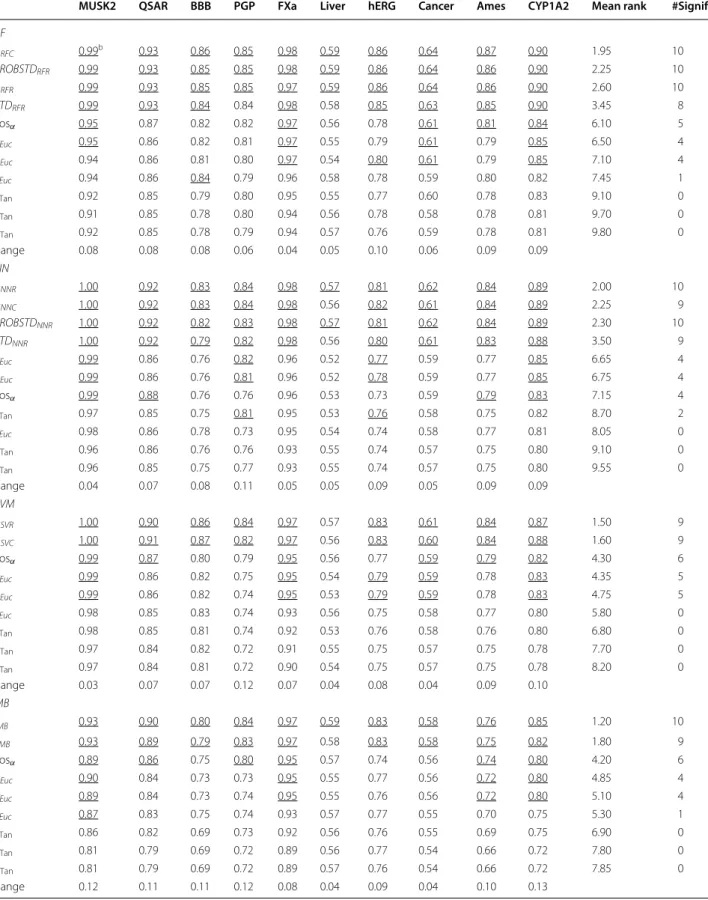
Table 2 AUC ROC for all classification techniques and AD measures
MUSK2 QSAR BBB PGP FXa Liver hERG Cancer Ames CYP1A2 Mean rank #Signif.a
RF ¯
pRFC 0.99b 0.93 0.86 0.85 0.98 0.59 0.86 0.64 0.87 0.90 1.95 10
PROBSTDRFR 0.99 0.93 0.85 0.85 0.98 0.59 0.86 0.64 0.86 0.90 2.25 10 ¯
pRFR 0.99 0.93 0.85 0.85 0.97 0.59 0.86 0.64 0.86 0.90 2.60 10
STDRFR 0.99 0.93 0.84 0.84 0.98 0.58 0.85 0.63 0.85 0.90 3.45 8
cosα 0.95 0.87 0.82 0.82 0.97 0.56 0.78 0.61 0.81 0.84 6.10 5
γEuc 0.95 0.86 0.82 0.81 0.97 0.55 0.79 0.61 0.79 0.85 6.50 4
κEuc 0.94 0.86 0.81 0.80 0.97 0.54 0.80 0.61 0.79 0.85 7.10 4
δEuc 0.94 0.86 0.84 0.79 0.96 0.58 0.78 0.59 0.80 0.82 7.45 1
δTan 0.92 0.85 0.79 0.80 0.95 0.55 0.77 0.60 0.78 0.83 9.10 0
γTan 0.91 0.85 0.78 0.80 0.94 0.56 0.78 0.58 0.78 0.81 9.70 0
κTan 0.92 0.85 0.78 0.79 0.94 0.57 0.76 0.59 0.78 0.81 9.80 0
Range 0.08 0.08 0.08 0.06 0.04 0.05 0.10 0.06 0.09 0.09
NN ¯
pNNR 1.00 0.92 0.83 0.84 0.98 0.57 0.81 0.62 0.84 0.89 2.00 10
¯
pNNC 1.00 0.92 0.83 0.84 0.98 0.56 0.82 0.61 0.84 0.89 2.25 9
PROBSTDNNR 1.00 0.92 0.82 0.83 0.98 0.57 0.81 0.62 0.84 0.89 2.30 10
STDNNR 1.00 0.92 0.79 0.82 0.98 0.56 0.80 0.61 0.83 0.88 3.50 9
γEuc 0.99 0.86 0.76 0.82 0.96 0.52 0.77 0.59 0.77 0.85 6.65 4
κEuc 0.99 0.86 0.76 0.81 0.96 0.52 0.78 0.59 0.77 0.85 6.75 4
cosα 0.99 0.88 0.76 0.76 0.96 0.53 0.73 0.59 0.79 0.83 7.15 4
δTan 0.97 0.85 0.75 0.81 0.95 0.53 0.76 0.58 0.75 0.82 8.70 2
δEuc 0.98 0.86 0.78 0.73 0.95 0.54 0.74 0.58 0.77 0.81 8.05 0
κTan 0.96 0.86 0.76 0.76 0.93 0.55 0.74 0.57 0.75 0.80 9.10 0
γTan 0.96 0.85 0.75 0.77 0.93 0.55 0.74 0.57 0.75 0.80 9.55 0
Range 0.04 0.07 0.08 0.11 0.05 0.05 0.09 0.05 0.09 0.09
SVM
ˆ
pSVR 1.00 0.90 0.86 0.84 0.97 0.57 0.83 0.61 0.84 0.87 1.50 9
ˆ
pSVC 1.00 0.91 0.87 0.82 0.97 0.56 0.83 0.60 0.84 0.88 1.60 9
cosα 0.99 0.87 0.80 0.79 0.95 0.56 0.77 0.59 0.79 0.82 4.30 6
γEuc 0.99 0.86 0.82 0.75 0.95 0.54 0.79 0.59 0.78 0.83 4.35 5
κEuc 0.99 0.86 0.82 0.74 0.95 0.53 0.79 0.59 0.78 0.83 4.75 5
δEuc 0.98 0.85 0.83 0.74 0.93 0.56 0.75 0.58 0.77 0.80 5.80 0
δTan 0.98 0.85 0.81 0.74 0.92 0.53 0.76 0.58 0.76 0.80 6.80 0
κTan 0.97 0.84 0.82 0.72 0.91 0.55 0.75 0.57 0.75 0.78 7.70 0
γTan 0.97 0.84 0.81 0.72 0.90 0.54 0.75 0.57 0.75 0.78 8.20 0
Range 0.03 0.07 0.07 0.12 0.07 0.04 0.08 0.04 0.09 0.10
MB ¯
fMB 0.93 0.90 0.80 0.84 0.97 0.59 0.83 0.58 0.76 0.85 1.20 10
ˆ
vMB 0.93 0.89 0.79 0.83 0.97 0.58 0.83 0.58 0.75 0.82 1.80 9
cosα 0.89 0.86 0.75 0.80 0.95 0.57 0.74 0.56 0.74 0.80 4.20 6
κEuc 0.90 0.84 0.73 0.73 0.95 0.55 0.77 0.56 0.72 0.80 4.85 4
γEuc 0.89 0.84 0.73 0.74 0.95 0.55 0.76 0.56 0.72 0.80 5.10 4
δEuc 0.87 0.83 0.75 0.74 0.93 0.57 0.77 0.55 0.70 0.75 5.30 1
δTan 0.86 0.82 0.69 0.73 0.92 0.56 0.76 0.55 0.69 0.75 6.90 0
γTan 0.81 0.79 0.69 0.72 0.89 0.56 0.77 0.54 0.66 0.72 7.80 0
κTan 0.81 0.79 0.69 0.72 0.89 0.57 0.76 0.54 0.66 0.72 7.85 0
bold in Table 2. The same clustering as in the case of the mean ranks can be found here. While confidence meas-ures generally produce rank orders that are significantly different from random rankings, this is often not the case for novelty measures.
Within the group of novelty measures the best per-forming AD measure is cosα followed by γEuc (i.e. the
mean distance to 5 nearest neighbors using Euclidean distance). Since the available confidence measures for each classifier vary, a single winner cannot be named. However, the type of confidence measure that constantly ranks first is always the same: it is either the built-in class probability estimate of the respective classification tech-nique or the class probability estimate from the related regression technique. For those classifiers without a regression counterpart (MB, k-NN, LDA), the built-in class probability estimate outperformed all other meas-ures (mainly novelty measmeas-ures). For those techniques that were run in classification and regression mode, the respective class probability estimates (i.e. pˆ and p¯) ranked top. In case of RF the classification mode has a slight edge while for NNs and SVMs the regression mode wins. However, the differences with respect to mean AUC ROC (across all data sets), mean rank and the num-ber of significant ROC curves are negligible. The same is
true for the ensemble-derived PROB-STD. It is also in the top ranking cluster for the two ensemble techniques (RF and NN). STD, which characterizes the ensemble stabil-ity, performs slightly worse.
In Table 2 it can be seen that the differences in AUC ROC between the best and worst AD measure for each data set given a particular classifier range between 0.04 (e.g. RF&FXa) and 0.13 (cf. MB&CYP1A2). The most fre-quent range is 0.09. The latter range, and thus the impact of the different AD measures, may be considered as rather small. However, the variation for a specific data set is exclusively due to different rankings of the predictions induced by the different AD measures. Please note, that there is a pattern in the ranges. If the classifier performs particularly well (i.e. NN&MUSK2, SVM&MUSK2) or particularly bad (Liver and Cancer data sets), the ranges tend to be small. For those data sets in between these extremes the range of AUC ROC is largest. That means that the impact of the different AD measures depends on the level of difficulty of the classification problem (expressed as AUC ROC) and will be largest for classifi-cation problems with intermediate difficulty (range AUC ROC: 0.7–0.9).
The performance of the different AD measures was also studied for different sets of structure descriptors (see a Number of data sets where the AD measure performs significantly better than chance based on the 95th percentile (α = 0.05) of the permutation test (see Additional file 1 for a description of the permutation test and Additional file 2 for code of the permutation test)
b Underlined values indicate that the AD measure performs significantly better than chance based on the permutation test (for details of the permutation test see also footnote a)
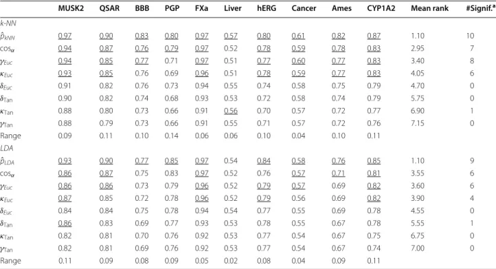
Table 2 continued
MUSK2 QSAR BBB PGP FXa Liver hERG Cancer Ames CYP1A2 Mean rank #Signif.a
k-NN
ˆ
pkNN 0.97 0.90 0.83 0.80 0.97 0.57 0.80 0.61 0.82 0.87 1.10 10
cosα 0.94 0.87 0.76 0.79 0.97 0.52 0.78 0.59 0.78 0.83 2.95 7
γEuc 0.94 0.85 0.77 0.71 0.97 0.51 0.77 0.60 0.77 0.83 3.40 8
κEuc 0.93 0.85 0.76 0.69 0.96 0.51 0.78 0.59 0.77 0.83 4.05 6
δEuc 0.91 0.82 0.76 0.73 0.94 0.55 0.74 0.58 0.75 0.79 4.70 0
δTan 0.90 0.82 0.74 0.68 0.93 0.53 0.72 0.58 0.74 0.79 5.75 0
κTan 0.88 0.80 0.73 0.66 0.91 0.56 0.70 0.57 0.72 0.77 6.90 1
γTan 0.88 0.79 0.73 0.66 0.91 0.55 0.71 0.57 0.72 0.76 7.15 0
Range 0.09 0.11 0.10 0.14 0.06 0.06 0.10 0.04 0.10 0.11
LDA
ˆ
pLDA 0.93 0.90 0.77 0.85 0.97 0.54 0.84 0.58 0.76 0.85 1.10 9
cosα 0.86 0.87 0.75 0.83 0.97 0.52 0.76 0.57 0.71 0.81 3.55 6
γEuc 0.86 0.86 0.73 0.79 0.96 0.52 0.79 0.57 0.69 0.82 3.60 6
κEuc 0.87 0.85 0.72 0.78 0.96 0.52 0.79 0.56 0.69 0.82 3.90 4
δEuc 0.84 0.84 0.75 0.78 0.94 0.54 0.77 0.55 0.69 0.78 4.55 0
δTan 0.86 0.83 0.69 0.77 0.93 0.53 0.78 0.55 0.67 0.78 5.55 1
κTan 0.82 0.81 0.70 0.76 0.92 0.53 0.77 0.54 0.67 0.75 6.75 0
γTan 0.82 0.81 0.69 0.76 0.92 0.53 0.77 0.54 0.67 0.74 7.00 0
Additional file 3: Tables S5–S10) and depending on the employed CV scheme (plain CV vs. RUS CV; see Addi-tional file 3: Tables S1, S2, S5–S7 for slightly imbalanced data sets). Summaries are given in Table S11 for different structure descriptors (CYP1A2) and in Table S12 for the two CV variants (QSAR, hERG). While the actual clas-sification performance sometimes changed, the best per-forming AD measures always remained the same, namely the built-in class probability estimates.
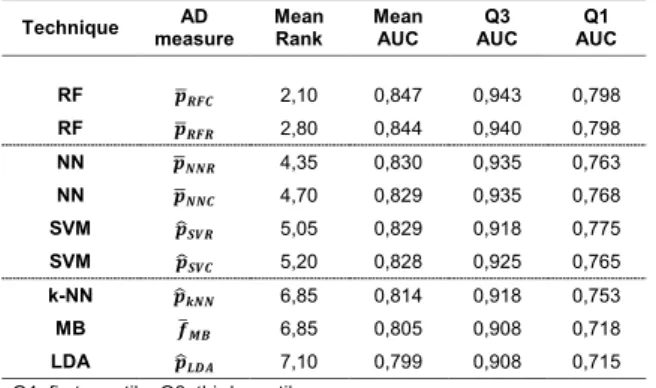
Thus far, the performance of different AD measures for a given classifier was studied which is the focus here. Next, we take a brief look at classifier performance. The AD measures derived from class probability estimates in classification and regression mode were analyzed. With one exception, where RF&PROBSTDRFR performed bet-ter than RF&p¯RFR for the FXa data set, they always per-formed best. Table 3 shows the mean rank and the mean AUC ROC. The single values for AUC ROC were taken from the respective line of Table 2. For the mean rank the nine different combinations were first ranked for each data set and afterwards the average rank over all data sets was taken, as it was for studying AD measure per-formance. Since the distribution of AUC ROC values is essentially trimodal, the first and the third quartile are given (there is no pattern in the median owing to this irregular distribution). It can be seen that there are three clusters in the data. The first is made up of the top rank-ing RFs, the second comprises NNs and SVMs, and the third consists of k-NN, MB and LDA. The same trend can be found in mean AUC ROC and the respective quartiles of AUC ROC.
Discussion
The employed AD measures can be differentiated into novelty measures and confidence measures. Novelty detection seeks to identify novel objects in sparsely
populated regions of the data set. Due to lacking near neighbors in the training set, it is assumed that these isolated objects are predicted with less reliability. How-ever, according to the results presented, the data density around a novel object does not very well predict the prob-ability of a prediction error. Basically, two different set-tings are conceivable: First, the novel object is located on the wrong side of the decision boundary since the latter is not well defined in that region where data are scarce. This is the standard assumption. Second, the novel object is isolated but on the correct side of the decision bound-ary, e.g. because it is in the tail of the data distribution pointing away from the decision boundary (i.e. it is iso-lated but far away from the decision boundary). Novelty detectors cannot differentiate these two cases, since they do not use the information of the class labels, they simply flag unusual objects. It follows that objects deemed novel need not show a larger error rate than those that are well embedded in the data. As a consequence, error rate reduction by rejecting the prediction of extreme objects is less efficient using novelty measures as compared to using confidence measures. This does not render novelty detectors useless. Novel objects may be interesting for a number of reasons, e.g. for detecting that novel chemical grounds were hit. However, novelty detection is simply not designed for error rate reduction since it does not use the most valuable resource in that respect: the class labels of the training set objects. Another reason why novelty detection performs worse in this study may be the curse of dimensionality since the employed structure descrip-tors are rather high-dimensional. Determining distances or data densities is notoriously difficult in high dimen-sions [72].
If novelty measures are to be used to flag extreme objects, cosα might be a reasonable choice. It ranked first behind the confidence measures in five out of six cases. Runner-up of the novelty measures was γEuc, which is
also a reasonable choice. However, it has to be borne in mind that this ranking was determined for AUC ROC und thus with a focus on error rate reduction which may not be the best criterion to assess novelty measures. Recently, specific benchmarks and criteria were studied for assessing the performance of different novelty meas-ures [73, 74]. Interestingly, the novelty measures based on Euclidean distance generally performed better than those using Tanimoto distance. While the differences in mean rank are sizeable, the absolute differences in AUC ROC tend to be small for the two measures. Moreover, most of the rankings according to novelty measures were not significantly different from chance so that it is not possible to draw a definite conclusion about their relative performance.
Confidence measures characterize the distance to the decision boundary. Not unexpectedly, the latter cor-relates far better with the error probability. Most of the built-in measures directly estimate the class probability (i.e. one minus the error probability). Ranking the data accordingly results in far better AUC ROC values and thus to a more efficient error rate reduction by rejecting the prediction of objects close to the decision boundary (see also below, predictiveness curves). The superior per-formance of class probability estimates is to be expected from the very purpose of these estimates. The idea of using class probability estimates for rejecting unreli-able predictions is everything but new (see [56, 75]) and class probability estimates are in widespread use in other related science fields (see e.g. [57, 76–79]). Yet, a sys-tematic evaluation of these measures for setting the AD in chemoinformatics was still missing. In the aforemen-tioned landmark collaborative study [9], the majority of confidence measures studied here was not included in that benchmark. Moreover, class probability estimates are not broadly applied for setting the AD in chemoin-formatics (for exceptions see e.g. [18, 80]). Certainly, con-formal prediction, which was recently introduced into chemoinformatics [24], follows a similar philosophy in estimating the reliability of a prediction (by a noncon-formity score) for rejecting its prediction if it is too unre-liable. As mentioned before, the results obtained here, are also of interest for choosing the nonconformity score. The conformal predictors published thus far in chemoin-formatics used confidence measures (either vj(xnew) for RFC or decval(xnew) for SVC) [24, 25, 27, 81]. While the latter two measures were not explicitly included in the benchmark here, the differences between vj(xnew) and
¯
pRFC are negligible for a reasonably large ensemble of trees and decval(xnew) is simply the uncalibrated version of pˆSVC where the calibration does not change the
perfor-mance of the conformal predictor. The results presented here support this careful choice of the nonconformity score.
Class probability measures can be derived from either classification or regression algorithms. In the two-class case studied here, there are slight differences between classification and regression mode but these are negli-gible for a practitioner. Hence, it is safe to recommend using the classification mode with the respective class probability estimate. Alternative confidence measures such as PROB-STD do perform almost as well as the top-ranking class probability estimate and for the practi-tioner there is little difference for choosing among them. Since the computation of PROB-STD needs a homo- or hetero-ensemble, it is in many cases more convenient to use the built-in class probability estimate since the lat-ter is computed in any case. It is also of note that STD,
which characterizes the stability of the ensemble, does not perform as well as the top-ranking class probability estimates. This is noteworthy since STD is the measure of choice in regression problems when the reliability of a predicted continuous variable (as opposed to a class probability estimate) shall be assessed [69, 82]. This could be explained as follows: The average output of a regres-sion ensemble is the estimate for the continuous response variable. It is well-known that using the ensemble average typically reduces the prediction error in regression prob-lems. Yet, the ensemble average does not characterize the reliability in regression. Therefore, the standard devia-tion of the ensemble output is used. In classificadevia-tion, the ensemble average (of the class probability estimate) can directly be used to characterize the reliability of the individual prediction. Using the standard deviation of the ensemble output is not necessary but yields slightly inferior results as compared to the average output of the ensemble (i.e. p¯ for RFs and NNs).
The accuracy, and thus AUC ROC, varies across the data sets. Despite this variation, class probability esti-mates always perform best. However, it has been shown that the gain in AUC ROC depends on the level of dif-ficulty (expressed as AUC ROC). For very difficult clas-sification problems with a high error rate reliable confidence estimation would be most desirable. Yet, in cases where the base classifier does not work well, the class probability estimates are also unreliable. Conse-quently, the gain in AUC ROC over a random ranking
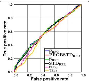
Fig. 1 Liver data set employing classification random forests. Receiver operating characteristic (ROC) curves are shown for all confidence measures and the two novelty measures cosα and γEuc.
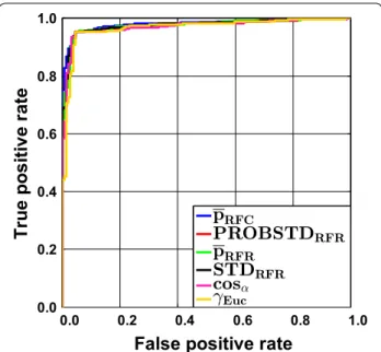
is small. This is illustrated for RF in Fig. 1 for the Liver data set. All ROC curves for this data set are very similar and no notable gain in AUC over a random ranking can be obtained. This shows that it is not possible to enrich the correct predictions at the top and at the end of the ranking list. As a consequence, error rate reduction will rather be negligible when a reject option is employed, even if the best classifier and the best AD measure are chosen. The gain will also be small for very easy clas-sification problems. This is illustrated in Fig. 2 for the FXa data in combination with RF. In this case only few errors occur and the class assignment will be unequivo-cal in most cases. As a consequence of the low error rate, differences between the ideal ROC curve and a ROC curve with a random ranking will be small. Using sim-ple geometric arguments, it is easy to show that the AUC obtained by randomly ranking the prediction errors (i.e. the median of the permutation distribution) corresponds to AUCrandom=0.5·(Sens+Spec) and the best possible AUC would be AUCmax=1−((1−Sens)·(1−Spec)) , where Sens and Spec are the abbreviations for the sen-sitivity and the specificity of a classifier, respectively. RF using RUS CV results in a sensitivity of 0.953 and a specificity of 0.955 for the FXa data set (Additional file 3: Table S5). In this case even a random ranking of the prediction errors results in an AUC ROC of 0.954, the maximum obtainable AUC ROC would be 0.998. It can be seen that large differences between a random ranking
and the ranking according to the optimal class probability estimate will be small. Please recall that we used the 95th percentile of the permutation distribution for assessing the significance of the ranking. That means that a rank-ing is considered significant only, if it yields a larger AUC ROC than AUCrandom. The actual amount depends on the data set.
The largest impact of applying the ideal AD meas-ure is expected for intermediately difficult classification problems. This is illustrated in Fig. 3 which shows the RF results for the Ames data set. Here, two clusters of ROC curves can be seen. The set of curves ascending steeper at the beginning belongs to the confidence measures and yield larger AUC ROC values. The curves resulting from novelty measures run more or less linearly from and to the point [1−Spec, Sens] which reflects a random order-ing of the prediction errors. The AUC ROC values for the different sets of curves vary notably. The class prob-ability estimates are rather reliable in this case and can make a difference as compared to randomly ranking the data. This is corroborated by the AUCrandom and AUCmax values. Random forest classifies the data with a sensitivity of 0.823 and a specificity of 0.770 (see Additional file 3: Table S9) which yields an AUCrandom of 0.797 and an
AUCmax of 0.959. The actual AUC ROC of RF&p¯RFC is 0.87. It can be seen that a gain of approximately 0.08 over
Fig. 2 FXa data set employing classification random forests. Receiver operating characteristic (ROC) curves are shown for all confidence measures and the two novelty measures cosα and γEuc. The overall accuracy is extremely high. Consequently, the gain in AUC ROC with the optimal AD measure is limited (for details see text)
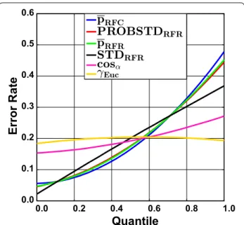
AUCrandom can be obtained. Yet, the actual AUC is still away from the ideal one. Since class probability estimates will always be inaccurate in real world applications, it is unrealistic to expect AUC values close to AUCmax except for trivial cases. In any case, this example shows that error rate reduction by employing a reject option will have an impact for the intermediate cases. This is illus-trated in Figs. 4 and 5 where the cumulative accuracy (CA) and predictiveness curves for RF and the Ames data set are shown. In a cumulative accuracy curve, the accuracy for predictions up to the ν th quantile of the AD measure is plotted against the quantile ν (or the percent-age of data, respectively). For the CA plots the same two clusters as in the case of ROC curves can be seen. For novelty measures, the CA plot show that only few reliable predictions can be sorted to the top of the ranking list and thus they start lower than the confidence measures and decrease quickly. In a predictiveness curve the error rate associated with the νth quantile of the AD measure is plotted against the quantile ν. If the AD measure per-forms well, the error at the beginning of the curve will be small while it should be far larger at the end. A sig-nificant slope between the error rate and the AD measure can only be found for the confidence measures, while for the novelty measures the slope is small or insignificant. It can be seen that there is a sharp increase in error rate for the extreme 10–20% of the data when the confidence measures are used as AD measures. For instance, local
error rates above 0.3 can largely be avoided if the rejec-tion threshold is set to the 80% quantile of the confidence measures. It can also be seen that the first 30% of the data can be predicted with a local error rate below 0.1 using
¯
pRFC, p¯RFR, or PROBSTDRFR. In summary, predictiveness curves display the local error rates of the different AD measures, which is well suited to assess the gain that can be obtained with a particular AD measure. While local error rates are very intuitive, no differentiation of FP and FN is possible like in the case of CA curves. This is of par-ticular importance for unbalanced data sets. If no action is taken to re-balance the training of the classifier, predic-tiveness curves as well as CA plots may be misleading. Since ROC curves are not affected by the class portions it is safer to use them. However, they do not display infor-mation about overall or local error rates. Moreover, it has been shown that the differences between AUCrandom and the AUC of the best performing combination of classifier and AD measure tend to be small which requires careful interpretation of the results. Finally, all three curves allow to reliably identify those AD measures that do not per-form better than chance.
Conclusion
The goal of defining an AD in classification problems is to identify the region in chemical space where “the model makes predictions with a given reliability”. This goal can be achieved in two fundamentally different ways. Fig. 4 Ames data set employing classification random forests. Cumu‑
lative accuracy (CA) curves are shown for all confidence measures and the two novelty measures cosα and γEuc. As with ROC curves, the inferior performance of the novelty measures can easily be seen. CA curves allow reading out the overall accuracy obtained when only a portion of x% of the data is predicted and the rest is rejected
Fig. 5 Ames data set employing classification random forests. Pre‑ dictiveness curves for all confidence measures and the two novelty measures cosα and γEuc are shown. They show the dependence of
First, unusual objects can be flagged assuming that they are likely outside the aforementioned region. This was referred to as novelty detection here. Second, unreliable predictions can be flagged which was referred to as con-fidence estimation. If error rate reduction is the focus of defining an AD, it is mandatory to use confidence meas-ures for defining the AD. Confidence measmeas-ures will iden-tify objects that are close to the decision boundary and will reject to predict them, which in turn reduces the error rate. From the confidence measures, the built-in class probability estimates performed constantly best, irrespective of the difficulty of the classification problem. Ideal class probability estimates for the studied model-ling techniques are listed in Table 3. Alternatives to class probability estimates do not perform better and are infe-rior in other cases. In the two-class case studied here, differences between learning a classification problem and training a regression algorithm with a dichotomous response variable could not be found. For the sake of sim-plicity, the general recommendation for efficiently defin-ing the AD would be to train a powerful classifier and use its built-in class probability estimate. In this study ran-dom forests once more proved to solve predictive chem-oinformatic modelling tasks best. Hence, classification random forests using p¯RFC as built-in confidence meas-ure are a good starting point for defining the AD.
Abbreviations
AD: applicability domain; AUC: area under the curve; AUC ROC: area under the receiver operating characteristic curve; CV: cross‑validation; DM: distance to model; k‑NN: k‑nearest neighbor; LDA: linear discriminant analysis; MB: multiple boosting; MOE: molecular operating environment; NN: neural net‑ works; NNC: classification neural networks; NNR: regression neural networks; PDF: probability density function; Q1: first quartile; Q3: third quartile; QSAR: quantitative structure–activity relationship; RF: random forests; RFC: classifica‑ tion random forests; RFR: regression random forests; ROC: receiver operating characteristic; RUS: random undersampling; SVC: support vector classification; SVM: support vector machines; SVR: support vector regression.
Additional files
Additional file 1. Detailed information about the classification methods, model validation, benchmarking criteria, the comparison between ROC and CA curves and the influence of RUS CV on ROC curves of novelty measures.
Additional file 2. Matlab‑code for permutation test to determine the distribution of AUC ROC values under the null hypothesis that the AD measure does not carry any information.
Additional file 3. Figures of merit (sensitivity, specificity, accuracy, AUC ROC) for all data sets with all CV variants on all descriptors sets (Tables S1–S10). Influence of different descriptor sets for CYP1A2 data set (Table S11). Influence of CV variant for QSAR and hERG data sets (Table S12). MOE descriptors (Table S13).
Additional file 4. Source of the data.
Additional file 5. Data sets used in this study. The data are provided in the way they were used for the respective computations. In addition to the data, the indices for the fivefold CV are also provided.
Authors’ contributions
KB, WK, MM conceived and designed the study. WK and MM performed the experiments. All authors analyzed the data. KB, WK, MM wrote the manuscript. All authors read and approved the final manuscript.
Author details
1 Institute of Medicinal and Pharmaceutical Chemistry, University of Technol‑ ogy Braunschweig, Beethovenstrasse 55, 38106 Brunswick, Germany. 2 Bayer Pharma Aktiengesellschaft, Computational Chemistry, Müllerstrasse 178, 13353 Berlin, Germany.
Acknowledgements
We thank the referees for helpful comments.
Competing interests
The authors declare that they have no competing interests.
Availability of data and materials
All data sets are included in the supplementary material as Additional file 5.
Funding
No third party funding was received.
Publisher’s Note
Springer Nature remains neutral with regard to jurisdictional claims in pub‑ lished maps and institutional affiliations.
Received: 30 November 2016 Accepted: 13 July 2017
References
1. Todeschini R, Consonni V (2009) Molecular descriptors for chemoinfor‑ matics, 2nd edn. Wiley, Weinheim
2. Hansch C, Fujita T (1964) p ‑σ‑π analysis. A method for the correlation of biological activity and chemical structure. J Am Chem Soc 86:1616–1626. doi:10.1021/ja01062a035
3. Hand DJ, Mannila H, Smyth P (2001) Principles of data mining. MIT Press, Cambridge
4. Murphy KP (2012) Machine learning. A probabilistic perspective. MIT Press, Cambridge
5. Netzeva TI, Worth A, Aldenberg T, Benigni R, Cronin MTD, Gramatica P, Jaworska JS, Kahn S, Klopman G, Marchant CA, Myatt G, Nikolova‑Jeli‑ azkova N, Patlewicz GY, Perkins R, Roberts D, Schultz T, Stanton DW, van de Sandt JM, Tong W, Veith G, Yang C (2005) Current status of methods for defining the applicability domain of (quantitative) structure‑activity relationships. Altern Lab Anim 33:155–173
6. OECD (2014) Guidance document on the validation of (quantitative) structure‑activity relationship [(Q)SAR] models. OECD Publishing, Paris. doi:10.1787/20777876
7. Sheridan RP, Feuston BP, Maiorov VN, Kearsley SK (2004) Similarity to mol‑ ecules in the training set is a good discriminator for prediction accuracy in QSAR. J Chem Inf Model 44:1912–1928. doi:10.1021/ci049782w 8. Chandola V, Banerjee A, Kumar V (2009) Anomaly detection. ACM Com‑
put Surv 41:1–58. doi:10.1145/1541880.1541882
9. Sushko I, Novotarskyi S, Körner R, Pandey AK, Cherkasov A, Li J, Gramatica P, Hansen K, Schroeter T, Müller K‑R, Xi L, Liu H, Yao X, Öberg T, Hor‑ mozdiari F, Dao P, Sahinalp C, Todeschini R, Polishchuk P, Artemenko A, Kuz’min V, Martin TM, Young DM, Fourches D, Muratov E, Tropsha A, Baskin I, Horvath D, Marcou G, Muller C, Varnek A, Prokopenko VV, Tetko IV (2010) Applicability domains for classification problems: benchmark‑ ing of distance to models for Ames mutagenicity set. J Chem Inf Model 50:2094–2111. doi:10.1021/ci100253r