Automatic Photo Pop-up
Derek Hoiem Alexei A. Efros Martial Hebert
Carnegie Mellon University
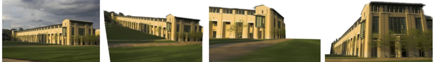
Figure 1: Our system automatically constructs a rough 3D environment from a single image by learning a statistical model of geometric classes from a set of training images. A photograph of the University Center at Carnegie Mellon is shown on the left, and three novel views from an automatically generated 3D model are to its right.
Abstract
This paper presents a fully automatic method for creating a 3D model from a single photograph. The model is made up of sev-eral texture-mapped planar billboards and has the complexity of a typical children’s pop-up book illustration. Our main insight is that instead of attempting to recover precise geometry, we statistically modelgeometric classesdefined by their orientations in the scene. Our algorithm labels regions of the input image into coarse cate-gories: “ground”, “sky”, and “vertical”. These labels are then used to “cut and fold” the image into a pop-up model using a set of sim-ple assumptions. Because of the inherent ambiguity of the problem and the statistical nature of the approach, the algorithm is not ex-pected to work on every image. However, it performs surprisingly well for a wide range of scenes taken from a typical person’s photo album.
CR Categories: 1.3.7 [Computer Graphics]: Three-Dimensional Graphics and Realism—Color, shading, shadowing, and texture 1.4.8 [Image Processing and Computer Vision]: Scene Analysis— Surface Fitting;
Keywords: image-based rendering, single-view reconstruction, machine learning, image segmentation
1
Introduction
Major advances in the field of image-based rendering during the past decade have made the commercial production of virtual models from photographs a reality. Impressive image-based walkthrough environments can now be found in many popular computer games and virtual reality tours. However, the creation of such environ-ments remains a complicated and time-consuming process, often
{dhoiem,efros,hebert}@cs.cmu.edu
Robotics Institute, Carnegie Mellon University, Pittsburgh, PA 15213, USA. http://www.cs.cmu.edu/∼dhoiem/projects/popup/
requiring special equipment, a large number of photographs, man-ual interaction, or all three. As a result, it has largely been left to the professionals and ignored by the general public.
We believe that many more people would enjoy the experience of virtually walking around in their own photographs. Most users, however, are just not willing to go through the effort of learning a new interface and taking the time to manually specify the model for each scene. Consider the case of panoramic photo-mosaics: the underlying technology for aligning photographs (manually or semi-automatically) has been around for years, yet only the availability of fully automatic stitching tools has really popularized the practice. In this paper, we present a method for creating virtual walkthroughs that iscompletely automaticand requires onlya single photograph
as input. Our approach is similar to the creation of a pop-up illus-tration in a children’s book: the image is laid on the ground plane and then the regions that are deemed to be vertical are automatically “popped up” onto vertical planes. Just like the paper pop-ups, our resulting 3D model is quite basic, missing many details. Nonethe-less, a large number of the resulting walkthroughs look surprisingly realistic and provide a fun “browsing experience” (Figure 1). The target application scenario is that the photos would be processed as they are downloaded from the camera into the com-puter and the users would be able to browse them using a 3D viewer (we use a simple VRML player) and pick the ones they like. Just like automatic photo-stitching, our algorithm is not expected to work well on every image. Some results would be incorrect, while others might simply be boring. This fits the pattern of modern dig-ital photography – people take lots of pictures but then only keep a few “good ones”. The important thing is that the user needs only to decide whether to keep the image or not.
1.1 Related Work
The most general image-based rendering approaches, such as Quicktime VR [Chen 1995], Lightfields [Levoy and Hanrahan 1996], and Lumigraph [Gortler et al. 1996] all require a huge num-ber of photographs as well as special equipment. Popular urban modeling systems such as Fac¸ade [Debevec et al. 1996], Photo-Builder [Cipolla et al. 1999] and REALVIZ ImageModeler greatly reduce the number of images required and use no special equipment (although cameras must still be calibrated), but at the expense of considerable user interaction and a specific domain of applicability. Several methods are able to perform user-guided modeling from a
(a) input image (b) superpixels (c) constellations (d) labeling (e) novel view Figure 2: 3D Model Estimation Algorithm. To obtain useful statistics for modeling geometric classes, we must first find uniformly-labeled regions in the image by computing superpixels (b) and grouping them into multiple constellations (c). We can then generate a powerful set of statistics and label the image based on models learned from training images. From these labels, we can construct a simple 3D model (e) of the scene. In (b) and (c), colors distinguish between separate regions; in (d) colors indicate the geometric labels: ground, vertical, and sky. single image. [Liebowitz et al. 1999; Criminisi et al. 2000] offer
the most accurate (but also the most labor-intensive) approach, re-covering a metric reconstruction of an architectural scene by using projective geometry constraints [Hartley and Zisserman 2004] to compute 3D locations of user-specified points given their projected distances from the ground plane. The user is also required to spec-ify other constraints such as a square on the ground plane, a set of parallel “up” lines and orthogonality relationships. Most other ap-proaches forgo the goal of a metric reconstruction, focusing instead on producing perceptually pleasing approximations. [Zhang et al. 2001] models free-form scenes by letting the user place constraints, such as normal directions, anywhere on the image plane and then optimizing for the best 3D model to fit these constraints. [Ziegler et al. 2003] finds the maximum-volume 3D model consistent with multiple manually-labeled images. Tour into the Picture[Horry et al. 1997], the main inspiration for this work, models a scene as an axis-aligned box, a sort of theater stage, with floor, ceiling, backdrop, and two side planes. An intuitive “spidery mesh” inter-face allows the user to specify the coordinates of this box and its vanishing point. Foreground objects are manually labeled by the user and assigned to their own planes. This method produces im-pressive results but works only on scenes that can be approximated by a one-point perspective, since the front and back of the box are assumed to be parallel to the image plane. This is a severe limita-tion (that would affect most of the images in this paper, including Figure 1(left)) which has been partially addressed by [Kang et al. 2001] and [Oh et al. 2001], but at the cost of a less intuitive inter-face.
Automatic methods exist to reconstruct certain types of scenes from multiple images or video sequences (e.g. [Nist´er 2001; Pollefeys et al. 2004]), but, to the best of our knowledge, no one has yet attempted automatic single-view modeling.
1.2 Intuition
Consider the photograph in Figure 1(left). Humans can easily grasp the overall structure of the scene – sky, ground, relative positions of major landmarks. Moreover, we can imagine reasonably well what this scene would look like from a somewhat different viewpoint, even if we have never been there. This is truly an amazing ability considering that, geometrically speaking, a single 2D image gives rise to an infinite number of possible 3D interpretations! How do we do it?
The answer is that our natural world, despite its incredible richness and complexity, is actually a reasonably structured place. Pieces of solid matter do not usually hang in mid-air but are part of surfaces that are usually smoothly varying. There is a well-defined notion of orientation (provided by gravity). Many structures exhibit high degree of similarity (e.g. texture), and objects of the same class tend to have many similar characteristics (e.g. grass is usually green and can most often be found on the ground). So, while an image
offers infinitely many geometrical interpretations, most of them can be discarded because they are extremely unlikely given what we know about our world. This knowledge, it is currently believed, is acquired through life-long learning, so, in a sense, a lot of what we consider human vision is based on statistics rather than geometry. One of the main contributions of this paper lies in posing the classic problem of geometric reconstruction in terms of statistical learning. Instead of trying to explicitly extract all the required geometric pa-rameters from a single image (a daunting task!), our approach is to rely on other images (the training set) to furnish this information in an implicit way, through recognition. However, unlike most scene recognition approaches which aim to model semantic classes, such as cars, vegetation, roads, or buildings [Everingham et al. 1999; Konishi and Yuille 2000; Singhal et al. 2003], our goal is to model
geometric classesthat depend on the orientation of a physical ob-ject with relation to the scene. For instance, a piece of plywood lying on the ground and the same piece of plywood propped up by a board have two different geometric classes but the same semantic class. We produce a statistical model of geometric classes from a set of labeled training images and use that model to synthesize a 3D scene given a new photograph.
2
Overview
We limit our scope to dealing with outdoor scenes (both natural and man-made) and assume that a scene is composed of a single ground plane, piece-wise planar objects sticking out of the ground at right angles, and the sky. Under this assumption, we can construct a coarse, scaled 3D model from a single image by classifying each pixel as ground, vertical or sky and estimating the horizon position. Color, texture, image location, and geometric features are all useful cues for determining these labels. We generate as many potentially useful cues as possible and allow our machine learning algorithm (decision trees) to figure out which to use and how to use them. Some of these cues (e.g., RGB values) are quite simple and can be computed directly from pixels, but others, such as geometric features require more spatial support to be useful. Our approach is to gradually build our knowledge of scene structure while being careful not to commit to assumptions that could prevent the true solution from emerging. Figure 2 illustrates our approach. Image to Superpixels
Without knowledge of the scene’s structure, we can only compute simple features such as pixel colors and filter responses. The first step is to find nearly uniform regions, called “superpixels” (Figure 2(b)), in the image. The use of superpixels improves the efficiency and accuracy of finding large single-label regions in the image. See Section 4.1 for details.
Superpixels to Multiple Constellations
can compute distributions of color and texture. To compute more complex features, we form groups of superpixels, which we call “constellations” (Figure 2(c)), that are likely to have the same label (based on estimates obtained from training data). These constel-lations span a sufficiently large portion of the image to allow the computation of all potentially useful statistics. Ideally, each con-stellation would correspond to a physical object in the scene, such as a tree, a large section of ground, or the sky. We cannot guarantee, however, that a constellation will describe a single physical object or even that all of its superpixels will have the same label. Due to this uncertainty, we generate several overlapping sets of possible constellations (Section 4.2) and use all sets to help determine the final labels.
Multiple Constellations to Superpixel Labels
The greatest challenge of our system is to determine the geomet-ric label of an image region based on features computed from its appearance. We take a machine learning approach, modeling the appearance of geometric classes from a set of training images. For each constellation, we estimate the likelihood of each of the three possible labels (“ground”, “vertical”, and “sky”) and the confidence that all of the superpixels in the constellation have the same label. Each superpixel’s label is then inferred from the likelihoods of the constellations that contain that superpixel (Section 4.3).
Superpixel Labels to 3D Model
We can construct a 3D model of a scene directly from the geometric labels of the image (Section 5). Once we have found the image pixel labels (ground, vertical, or sky), we can estimate where the objects lie in relation to the ground by fitting the boundary of the bottom of the vertical regions with the ground. The horizon position is estimated from geometric features and the ground labels. Given the image labels, the estimated horizon, and our single ground plane assumption, we can map all of the ground pixels onto that plane. We assume that the vertical pixels correspond to physical objects that stick out of the ground and represent each object with a small set of planar billboards. We treat sky as non-solid and remove it from our model. Finally, we texture-map the image onto our model (Figure 2(e)).
3
Features for Geometric Classes
We believe that color, texture, location in the image, shape, and pro-jective geometry cues are all useful for determining the geometric class of an image region (see Table 1 for a complete list).
Coloris valuable in identifying the material of a surface. For in-stance, the sky is usually blue or white, and the ground is often green (grass) or brown (dirt). We represent color using two color spaces: RGB and HSV (sets C1-C4 in Table 1). RGB allows the “blueness” or “greenness” of a region to be easily extracted, while HSV allows perceptual color attributes such as hue and “grayness” to be measured.
Textureprovides additional information about the material of a sur-face. For example, texture helps differentiate blue sky from wa-ter and green tree leaves from grass. Texture is represented using derivative of oriented Gaussian filters (sets T1-T4) and the 12 most mutually dissimilar of the universal textons (sets T5-T7) from the Berkeley segmentation dataset [Martin et al. 2001].
Locationin the image also provides strong cues for distinguishing between ground (tends to be low in the image), vertical structures, and sky (tends to be high in the image). We normalize the pixel locations by the width and height of the image and compute the mean (L1) and 10thand 90thpercentile (L2) of the x- and y-location of a region in the image. Additionally, region shape (L4-L7) helps
Feature Descriptions Num Used
Color 15 15
C1. RGB values: mean 3 3
C2. HSV values: conversion from mean RGB values 3 3 C3. Hue: histogram (5 bins) and entropy 6 6 C4. Saturation: histogram (3 bins) and entropy 3 3
Texture 29 13
T1. DOOG Filters: mean abs response 12 3 T2. DOOG Filters: mean of variables in T1 1 0 T3. DOOG Filters: id of max of variables in T1 1 1 T4. DOOG Filters: (max - median) of variables in T1 1 1 T5. Textons: mean abs response 12 7 T6. Textons: max of variables in T5 1 0 T7. Textons: (max - median) of variables in T5 1 1
Location and Shape 12 10
L1. Location: normalized x and y, mean 2 2 L2. Location: norm. x and y, 10thand 90thpercentile 4 4 L3. Location: norm. y wrt horizon, 10thand 90thpctl 2 2 L4. Shape: number of superpixels in constellation 1 1 L5. Shape: number of sides of convex hull 1 0 L6. Shape:num pixels/area(convex hull) 1 1 L7. Shape: whether the constellation region is contiguous 1 0
3D Geometry 35 28
G1. Long Lines: total number in constellation region 1 1 G2. Long Lines: % of nearly parallel pairs of lines 1 1 G3. Line Intersection: hist. over 12 orientations, entropy 13 11 G4. Line Intersection: % right of center 1 1 G5. Line Intersection: % above center 1 1 G6. Line Intersection: % far from center at 8 orientations 8 4 G7. Line Intersection: % very far from center at 8 orientations 8 5 G8. Texture gradient: x and y “edginess” (T2) center 2 2
Table 1: Features for superpixels and constellations. The “Num” column gives the number of variables in each set. The simpler fea-tures (sets C1-C2,T1-T7, and L1) are used to represent superpix-els, allowing the formation of constellations over which the more complicated features can be calculated. All features are available to our constellation classifier, but the classifier (boosted decision trees) actually uses only a subset. Features may not be selected because they are not useful for discrimination or because their in-formation is contained in other features. The “Used” column shows how many variables from each set are actually used in the classifier. distinguish vertical regions (often roughly convex) from ground and sky regions (often non-convex and large).
3D Geometryfeatures help determine the 3D orientation of sur-faces. Knowledge of the vanishing line of a plane completely spec-ifies its 3D orientation relative to the viewer [Hartley and Zisser-man 2004], but such information cannot easily be extracted from outdoor, relatively unstructured images. By computing statistics of straight lines (G1-G2) and their intersections (G3-G7) in the image, our system gains information about the vanishing points of a surface without explicitly computing them. Our system finds long, straight edges in the image using the method of [Kosecka and Zhang 2002]. The intersections of nearly parallel lines (withinπ/8 radians) are radially binned, according to the direction to the intersection point from the image center (8 orientations) and the distance from the image center (thresholds of 1.5 and 5.0 times the image size). The texture gradient can also provide orientation cues even for natural surfaces without parallel lines. We capture texture gradient infor-mation (G8) by comparing a region’s center of mass with its center of “texturedness”.
We also estimate thehorizon positionfrom the intersections of nearly parallel lines by finding the position that minimizes theL12 -distance (chosen for its robustness to outliers) from all of the in-tersection points in the image. This often provides a reasonable estimate of the horizon in man-made images, since these scenes contain many lines parallel to the ground plane (thus having
van-ishing points on the horizon in the image). Feature set G3 relates the coordinates of the constellation region relative to the estimated horizon, which is often more relevant than the absolute image co-ordinates.
4
Labeling the Image
Many geometric cues become useful only when something is known about the structure of the scene. We gradually build our structural knowledge of the image, from pixels to superpixels to constellations of superpixels. Once we have formed multiple sets of constellations, we estimate the constellation label likelihoods and the likelihood that each constellation is homogeneously labeled, from which we infer the most likely geometric labels of the su-perpixels.
4.1 Obtaining Superpixels
Initially, an image is represented simply by a 2D array of RGB pixels. Our first step is to form superpixels from those raw pixel in-tensities. Superpixels correspond to small, nearly-uniform regions in the image and have been found useful by other computer vision and graphics researchers [Tao et al. 2001; Ren and Malik 2003; Li et al. 2004]. The use of superpixels improves the computational efficiency of our algorithm and allows slightly more complex sta-tistics to be computed for enhancing our knowledge of the image structure. Our implementation uses the over-segmentation tech-nique of [Felzenszwalb and Huttenlocher 2004].
4.2 Forming Constellations
Next, we group superpixels that are likely to share a common geo-metric label into “constellations”. Since we cannot be completely confident that these constellations are homogeneously labeled, we find multiple constellations for each superpixel in the hope that at least one will be correct. The superpixel features (color, texture, location) are not sufficient to determine the correct label of a super-pixel but often allow us to determine whether a pair of supersuper-pixels has the same label (i.e. belong in the same constellation).
To form constellations, we initialize by assigning one randomly se-lected superpixel to each ofNcconstellations. We then iteratively
assign each remaining superpixel to the constellation most likely to share its label, maximizing the average pairwise log-likelihoods with other superpixels in the constellation:
S(C) =
Nc
∑
k
1
nk(1−nk)i,
∑
j∈CklogP(yi=yj||zi−zj|) (1)
wherenkis the number of superpixels in constellationCk. P(yi= yj||zi−zj|)is the estimated probability that two superpixels have
the same label, given the absolute difference of their feature vectors (see Section 4.4 for how we estimate this likelihood from training data). By varying the number of constellations (from 3 to 25 in our implementation), we explore the trade-off of variance, from poor spatial support, and bias, from risk of mixed labels in a constella-tion.
4.3 Geometric Classification
For each constellation, we estimate the confidence in each geomet-ric label (label likelihood) and whether all superpixels in the
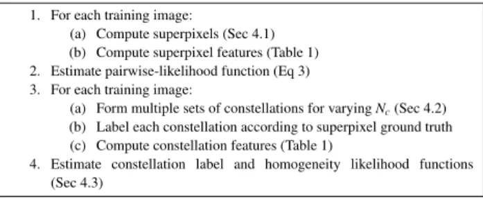
con-1. For each training image:
(a) Compute superpixels (Sec 4.1) (b) Compute superpixel features (Table 1) 2. Estimate pairwise-likelihood function (Eq 3) 3. For each training image:
(a) Form multiple sets of constellations for varyingNc(Sec 4.2) (b) Label each constellation according to superpixel ground truth (c) Compute constellation features (Table 1)
4. Estimate constellation label and homogeneity likelihood functions (Sec 4.3)
Figure 3: Training procedure.
stellation have the same label (homogeneity likelihood). We esti-mate the likelihood of a superpixel label by marginalizing over the constellation likelihoods1:
P(yi=t|x) =
∑
k:si∈CkP(yk=t|xk,Ck)P(Ck|xk) (2)
wheresi is theith superpixel and yi is the label of si. Each
su-perpixel is assigned its most likely label. Ideally, we would mar-ginalize over the exponential number of all possible constellations, but we approximate this by marginalizing over several likely ones (Section 4.2).P(yk=t|xk,Ck)is the label likelihood, andP(Ck|xk)
is the homogeneity likelihood for each constellationCkthat
con-tainssi. The constellation likelihoods are based on the featuresxk
computed over the constellation’s spatial support. In the next sec-tion, we describe how these likelihood functions are learned from training data.
4.4 Training Training Data
The likelihood functions used to group superpixels and label con-stellations are learned from training images. We gathered a set of 82 images of outdoor scenes (our entire training set with labels is avail-able online) that are representative of the images that users choose to make publicly available on the Internet. These images are often highly cluttered and span a wide variety of natural, suburban, and urban scenes. Each training image is over-segmented into super-pixels, and each superpixel is given a ground truth label according to its geometric class. The training process is outlined in Figure 3. Superpixel Same-Label Likelihoods
To learn the likelihoodP(yi=yj||zi−zj|) that two superpixels
have the same label, we sample 2,500 same-label and different-label pairs of superpixels from our training data. From this data, we estimate the pairwise likelihood function using the logistic re-gression form of Adaboost [Collins et al. 2002]. Each weak learner
fmis based on naive density estimates of the absolute feature
dif-ferences:
fm(z1,z2) = nf
∑
i
logPm(y1=y2,|z1i−z2i|) Pm(y16=y2,|z1i−z2i|)
(3) wherez1andz2are the features from a pair of superpixels,y1and y2are the labels of the superpixels, andnfis the number of features.
Each likelihood functionPmin the weak learner is obtained using
kernel density estimation [Duda et al. 2000] over themthweighted
distribution. Adaboost combines an ensemble of estimators to im-prove accuracy over any single density estimate.
Constellation Label and Homogeneity Likelihoods
To learn the label likelihoodP(yk=t|xk,Ck)and homogeneity
like-1This formulation makes the dubious assumption that there is only one
(a) Fitted Segments (b) Cuts and Folds Figure 4: From the noisy geometric labels, we fit line segments to the ground-vertical label boundary (a) and form those segments into a set of polylines. We then “fold” (red solid) the image along the polylines and “cut” (red dashed) upward at the endpoints of the polylines and at ground-sky and vertical-sky boundaries (b). The polyline fit and the estimated horizon position (yellow dotted) are sufficient to “pop-up” the image into a simple 3D model.
Partition the pixels labeled as vertical into connected regions For each connected vertical region:
1. Find ground-vertical boundary(x,y) locationsp
2. Iteratively find best-fitting line segmentsuntil no segment contains more thanmppoints:
(a) Find best lineLinpusing Hough transform
(b) Find largest set of pointspL∈pwithin distancedtofLwith no gap between consecutive points larger thangt
(c) RemovepLfromp
3. Form set of polylines from line segments
(a) Remove smaller of completely overlapping (in x-axis) segments (b) Sort segments by median of points on segment along x-axis (c) Join consecutive intersecting segments into polyline if the
inter-section occurs between segment medians (d) Remove smaller of any overlapping polylines Foldalong polylines
Cutupward from polyline endpoints, at ground-sky and vertical-sky boundaries Projectplanes into 3D coordinates and texture map
Figure 5: Procedure for determining the 3D model from labels. lihoodP(Ck|xk), we form multiple sets of constellations for the
su-perpixels in our training images using the learned pairwise func-tion. Each constellation is then labeled as “ground”, “vertical”, “sky”, or “mixed” (when the constellation contains superpixels of differing labels), according to the ground truth. The likelihood functions are estimated using the logistic regression version of Ad-aboost [Collins et al. 2002] with weak learners based on eight-node decision trees [Quinlan 1993; Friedman et al. 2000]. Each deci-sion tree weak learner selects the best features to use (based on the current weighted distribution of examples) and estimates the con-fidence in each label based on those features. To place emphasis on correctly classifying large constellations, the weighted distribu-tion is initialized to be propordistribu-tional to the percentage of image area spanned by each constellation.
The boosted decision tree estimator outputs a confidence for each of “ground”, “vertical”, “sky”, and “mixed”, which are normalized to sum to one. The product of the label and homogeneity likelihoods for a particular geometric label is then given by the normalized con-fidence in “ground”, “vertical”, or “sky”.
5
Creating the 3D Model
To create a 3D model of the scene, we need to determine the cam-era parameters and where each vertical region intersects the ground. Once these are determined, constructing the scene is simply a mat-ter of specifying plane positions using projective geometry and tex-ture mapping from the image onto the planes.
5.1 Cutting and Folding
We construct a simple 3D model by making “cuts” and “folds” in the image based on the geometric labels (see Figure 4). Our model consists of a ground plane and planar objects at right angles to the ground. Even given these assumptions and the correct labels, many possible interpretations of the 3D scene exist. We need to partition the vertical regions into a set of objects (especially difficult when objects regions overlap in the image) and determine where each ob-ject meets the ground (impossible when the ground-vertical bound-ary is obstructed in the image). We have found that, qualitatively, it is better to miss a fold or a cut than to make one where none exists in the true model. Thus, in the current implementation, we do not attempt to segment overlapping vertical regions, placing folds and making cuts conservatively.
As a pre-processing step, we set any superpixels that are labeled as ground or sky and completely surrounded by ground or non-sky pixels to the most common label of the neighboring superpixels. In our tests, this affects no more than a few superpixels per image but reduces small labeling errors (compare the labels in Figures 2(d) and 4(a)).
Figure 5 outlines the process for determining cuts and folds from the geometric labels. We divide the vertically labeled pixels into disconnected or loosely connected regions using the connected components algorithm (morphological erosion and dilation sepa-rate loosely connected regions). For each region, we fit a set of line segments to the region’s boundary with the labeled ground using the Hough transform [Duda and Hart 1972]. Next, within each re-gion, we form the disjoint line segments into a set of polylines. The pre-sorting of line segments (step 3(b)) and removal of overlapping segments (steps 3(a) and 3(d)) help make our algorithm robust to small labeling errors.
If no line segment can be found using the Hough transform, a single polyline is estimated for the region by a simple method. The poly-line is initialized as a segment from the left-most to the right-most boundary points. Segments are then greedily split to minimize the
L1-distance of the fit to the points, with a maximum of three seg-ments in the polyline.
We treat each polyline as a separate object, modeled with a set of connected planes that are perpendicular to the ground plane. The ground is projected into 3D-coordinates using the horizon position estimate and fixed camera parameters. The ground intersection of each vertical plane is determined by its segment in the polyline; its height is specified by the region’s maximum height above the seg-ment in the image and the camera parameters. To map the texture onto the model, we create a ground image and a vertical image, with non-ground and non-vertical pixels having alpha values of zero in each respective image. We feather the alpha band of the vertical image and output a texture-mapped VRML model that allows the user to explore his image.
5.2 Camera Parameters
To obtain true 3D world coordinates, we would need to know the intrinsic and extrinsic camera parameters. We can, however, create a reasonable scaled model by estimating the horizon line (giving the angle of the camera with respect to the ground plane) and setting the remaining parameters to constants. We assume zero skew and unit affine ratio, set the field of view to 0.768 radians (the focal length in EXIF metadata can be used instead of the default, when available), and arbitrarily set the camera height to 5.0 units (which affects only the scale of the model). The method for estimating the horizon is described in the Section 3. If the labeled ground appears above
Figure 6: Original image taken from results of [Liebowitz et al. 1999] and two novel views from the 3D model generated by our system. Since the roof in our model is not slanted, the model generated by Liebowitzet al. is slightly more accurate, but their model is manually specified, while ours is created fully automatically!
1. Image→superpixels via over-segmentation (Sec 4.1) 2. Superpixels→multiple constellations (Sec 4.2)
(a) For each superpixel: compute features (Sec 1)
(b) For each pair of superpixels: compute pairwise likelihood of same label
(c) Varying the number of constellations:
maximize average pairwise log-likelihoods within constellations (Eq 1)
3. Multiple constellations→superpixel labels (Sec 4.3) (a) For each constellation:
i. Compute features (Sec 1)
ii. For each label∈{ground, vertical, sky}: compute label likelihood
iii. Compute likelihood of label homogeneity
(b) For each superpixel: compute label confidences (Eq 2) and assign most likely label
4. Superpixel labels→3D model (Sec 5)
(a) Partition vertical regions into a set of objects (b) For each object: fit ground-object intersection with line (c) Create VRML models by cutting out sky and “popping up”
ob-jects from the ground
Figure 7: Creating a VRML model from a single image. the estimated position of the horizon, we abandon that estimate and assume that the horizon lies slightly above the highest ground pixel.
6
Implementation
Figure 7 outlines the algorithm for creating a 3D model from an im-age. We used Felzenszwalb’s [2004] publicly available code to gen-erate the superpixels and implemented the remaining parts of the algorithm using MATLAB. The decision tree learning and kernel density estimation was performed using weighted versions of the functions from the MATLAB Statistics Toolbox. We used twenty Adaboost iterations for the learning of the pairwise likelihood and geometric labeling functions. In our experiments, we setNcto each
of{3,4,5,6,7,9,12,15}. We have found our labeling algorithm to be fairly insensitive to parameter changes or small changes in the way that the image statistics are computed.
In creating the 3D model from the labels, we set the minimum num-ber of boundary points per segmentmptos/20, wheresis the
diag-onal length of the image. We set the minimum distance for a point to be considered part of a segmentdt tos/100 and the maximum
horizontal gap between consecutive pointsgt to the larger of the
segment length ands/20.
The total processing time for an 800x600 image is about 1.5 minutes using unoptimized MATLAB code on a 2.13GHz Athalon machine.
7
Results
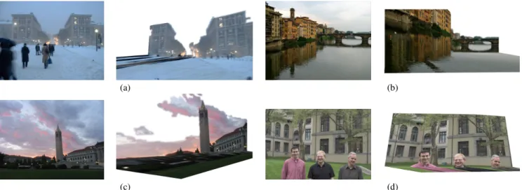
Figure 9 shows the qualitative results of our algorithm on several images. On a test set of 62 novel images, 87% of the pixels were correctly labeled into ground, vertical, or sky. Even when all pixels are correctly labeled, however, the model may still look poor if ob-ject boundaries and obob-ject-ground intersection points are difficult to determine. We found that about 30% of input images of outdoor scenes result in accurate models.
Figure 8 shows four examples of typical failures. Common causes of failure are 1) labeling error, 2) polyline fitting error, 3) model-ing assumptions, 4) occlusion in the image, and 5) poor estimation of the horizon position. Under our assumptions, crowded scenes (e.g. lots of trees or people) cannot be easily modeled. Addition-ally, our models cannot account for slanted surfaces (such as hills) or scenes that contain multiple ground-parallel planes (e.g. steps). Since we do not currently attempt to segment overlapping vertical regions, occluding foreground objects cause fitting errors or are ig-nored (made part of the ground plane). Additionally, errors in the horizon position estimation (our current method is quite basic) can cause angles between connected planes to be overly sharp or too shallow. By providing a simple interface, we could allow the user to quickly improve results by adjusting the horizon position, cor-recting labeling errors, or segmenting vertical regions into objects. Since the forming of constellations depends partly on a random ini-tialization, results may vary slightly when processing the same im-age multiple times. Increasing the number of sets of constellations would decrease this randomness at the cost of computational time.
8
Conclusion
We set out with the goal of automatically creating visually pleasing 3D models from a single 2D image of an outdoor scene. By making our small set of assumptions and applying a statistical framework to the problem, we find that we are able to create beautiful models for many images.
The problem of automatic single-view reconstruction, however, is far from solved. Future work could include the following improve-ments: 1) use segmentation techniques such as [Li et al. 2004] to improve labeling accuracy near region boundaries (our initial at-tempts at this have not been successful) or to segment out fore-ground objects; 2) estimate the orientation of vertical regions from the image data, allowing a more robust polyline fit; and 3) an ex-tension of the system to indoor scenes. Our approach to automatic single-view modeling paves the way for a new class of applications, allowing the user to add another dimension to the enjoyment of his photos.
(a) (b)
(c) (d)
Figure 8: Failures. Our system creates poor 3D models for these images. In (a) some foreground objects are incorrectly labeled as being in the ground plane; others are correctly labeled as vertical but are incorrectly modeled due to overlap of vertical regions in the image. In (b), the reflection of the building is mistaken for being vertical. Major labeling error in (c) results in a poor model. The failure (d) is due to the inability to segment foreground objects such as close-ups of people (even the paper authors).
Acknowledgments. The authors thank Rahul Sukthankar for many useful suggestions. We also thank the anonymous review-ers and Srinivas Narasimhan for their enormous help in revising the paper. We thank our photo contributors: James Hays (Fig-ures 1 and 8(d)); Todd Bliwise of http://www.trainweb.org/ toddsamtrakphotos(Figure 2); David Liebowitz (Figure 6); and Lana Lazebnik (Figure 9 top). Finally, AE thanks AZ and the rest of the Oxford group for convincing him that geometry is not dead after all.
References
CHEN, E. 1995. QuickTime VR - an image-based approach to virtual environment navigation. InACM SIGGRAPH 95, 29–38.
CIPOLLA, R., ROBERTSON, D.,ANDBOYER, E. 1999. Photobuilder – 3d models of architectural scenes from uncalibrated images. InIEEE Int. Conf. on Multimedia Computing and Systems, vol. I, 25–31.
COLLINS, M., SCHAPIRE, R.,ANDSINGER, Y. 2002. Logistic regression, adaboost and bregman distances.Machine Learning 48, 1-3, 253–285.
CRIMINISI, A., REID, I.,ANDZISSERMAN, A. 2000. Single view metrology. Int. Journal of Computer Vision 40, 2, 123–148.
DEBEVEC, P. E., TAYLOR, C. J.,ANDMALIK, J. 1996. Modeling and rendering architecture from photographs: A hybrid geometry- and image-based approach. In ACM SIGGRAPH 96, 11–20.
DUDA, R.,ANDHART, P. 1972. Use of the hough transformation to detect lines and curves in pictures.Communications of the ACM 15, 1, 11–15.
DUDA, R., HART, P., ANDSTORK, D. 2000. Pattern Classification. Wiley-Interscience Publication.
EVERINGHAM, M. R., THOMAS, B. T.,ANDTROSCIANKO, T. 1999. Head-mounted mobility aid for low vision using scene classification techniques. The Intl J. of Virtual Reality 3, 4, 3–12.
FELZENSZWALB, P.,ANDHUTTENLOCHER, D. 2004. Efficient graph-based image segmentation.Int. Journal of Computer Vision 59, 2, 167–181.
FRIEDMAN, J., HASTIE, T.,ANDTIBSHIRANI, R. 2000. Additive logistic regression: a statistical view of boosting.Annals of Statistics 28, 2, 337–407.
GORTLER, S. J., GRZESZCZUK, R., SZELISKI, R.,ANDCOHEN, M. F. 1996. The Lumigraph. InACM SIGGRAPH 96, 43–54.
HARTLEY, R. I.,ANDZISSERMAN, A. 2004.Multiple View Geometry in Computer Vision, 2nd ed. Cambridge University Press.
HORRY, Y., ANJYO, K.-I.,ANDARAI, K. 1997. Tour into the picture: using a spidery mesh interface to make animation from a single image. InACM SIGGRAPH 97, 225–232.
KANG, H., PYO, S., ANJYO, K.,ANDSHIN, S. 2001. Tour into the picture using a vanishing line and its extension to panoramic images. InProc. Eurographics, 132–141.
KONISHI, S.,ANDYUILLE, A. 2000. Statistical cues for domain specific image seg-mentation with performance analysis. InComputer Vision and Pattern Recognition, 1125–1132.
KOSECKA, J.,ANDZHANG, W. 2002. Video compass. InEuropean Conf. on Com-puter Vision, Springer-Verlag, 476–490.
LEVOY, M.,ANDHANRAHAN, P. 1996. Light field rendering. InACM SIGGRAPH 96, 31–42.
LI, Y., SUN, J., TANG, C.-K.,ANDSHUM, H.-Y. 2004. Lazy snapping.ACM Trans. on Graphics 23, 3, 303–308.
LIEBOWITZ, D., CRIMINISI, A.,ANDZISSERMAN, A. 1999. Creating architectural models from images. InProc. Eurographics, vol. 18, 39–50.
MARTIN, D., FOWLKES, C., TAL, D.,ANDMALIK, J. 2001. A database of human segmented natural images and its application to evaluating segmentation algorithms and measuring ecological statistics. InInt. Conf. on Computer Vision, vol. 2, 416– 423.
NISTER´ , D. 2001.Automatic dense reconstruction from uncalibrated video sequences. PhD thesis, Royal Institute of Technology KTH.
OH, B. M., CHEN, M., DORSEY, J.,ANDDURAND, F. 2001. Image-based modeling and photo editing. InACM SIGGRAPH 2001, ACM Press, 433–442.
POLLEFEYS, M., GOOL, L. V., VERGAUWEN, M., VERBIEST, F., CORNELIS, K., TOPS, J.,ANDKOCH, R. 2004. Visual modeling with a hand-held camera.Int. J. of Computer Vision 59, 3, 207–232.
QUINLAN, J. 1993. C4.5: Programs for Machine Learning. Morgan Kaufmann Publishers Inc.
REN, X.,ANDMALIK, J. 2003. Learning a classification model for segmentation. In Int. Conf. on Computer Vision, 10–17.
SINGHAL, A., LUO, J.,ANDZHU, W. 2003. Probabilistic spatial context models for scene content understanding. InComputer Vision and Pattern Recognition, 235– 241.
TAO, H., SAWHNEY, H. S.,ANDKUMAR, R. 2001. A global matching framework for stereo computation. InInt. Conf. on Computer Vision, 532–539.
ZHANG, L., DUGAS-PHOCION, G., SAMSON, J.,ANDSEITZ, S. 2001. Single view modeling of free-form scenes. InComputer Vision and Pattern Recognition, 990– 997.
ZIEGLER, R., MATUSIK, W., PFISTER, H.,ANDMCMILLAN, L. 2003. 3d recon-struction using labeled image regions. InEurographics Symposium on Geometry Processing, 248–259.

![Figure 6: Original image taken from results of [Liebowitz et al. 1999] and two novel views from the 3D model generated by our system.](https://thumb-us.123doks.com/thumbv2/123dok_us/8427747.2241795/6.918.93.835.81.225/figure-original-image-taken-results-liebowitz-novel-generated.webp)