Efficient Processing of Joins on Set-valued Attributes

(1)

Efficient Processing of Joins on Set-valued Attributes

Nikos Mamoulis

Department of Computer Science and Information Systems University of Hong Kong

Pokfulam Road Hong Kong nikos@csis.hku.hk

Abstract

Object-oriented and object-relational DBMS support set-valued attributes, which are a natural and concise way to model complex information. However, there has been lim-ited research to-date on the evaluation of query operators that apply on sets. In this paper we study the join of two relations on their set-valued attributes. Various join types are considered, namely the set containment, set equality, and set overlap joins. We show that the inverted file, a powerful index for selection queries, can also facilitate the efficient evaluation of most join predicates. We propose join algorithms that utilize inverted files and compare them with signature-based methods for several set-comparison predi-cates.

1. Introduction

Commercial object-oriented and object relational DBMS [14] support set-valued attributes in relations, which are a nat-ural and concise way to model complex information. Al-though sets are ubiquitous in many applications (document retrieval, semi-structured data management, data mining, etc.), there has been limited research on the evaluation of database operators that apply on sets.

On the other hand, there has been significant research in the IR community on the management of set-valued data, triggered by the need for fast content-based retrieval in doc-ument databases. Research in this area has focused on pro-cessing of keyword-based selection queries. A range of in-dexing methods has been proposed, among which signature-based techniques [2, 3, 9] and inverted files [16, 17] dominate. These indexes have been extensively revised and evaluated for various selection queries on set-valued attributes [15, 8]. An important operator which has received limited atten-tion is the join between two relaatten-tions on their set-valued attributes. Formally, given two relationsRandS, with set-valued attributesR.rand S.s,R1rθsS returns the subset of their Cartesian productR×S, in which the set-valued attributes qualify the join predicateθ. Two join operators

Permission to make digital or hard copies of all or part of this work for personal or classroom use is granted without fee provided that copies are not made or distributed for profit or commercial advantage and that copies bear this notice and the full citation on the first page. To copy otherwise, to republish, to post on servers or to redistribute to lists, requires prior specific permission and/or a fee.

that have been studied to date are theset containmentjoin, whereθ is⊆[7, 13], and theall nearest neighbors operator [11], which retrieves for each set inRitsknearest neighbors inSbased on a similarity function. Other operators include theset equalityjoin and theset overlapjoin.

As an example of a set containment join, consider the join of a job-offers relationRwith a persons relationSsuch that R.required skills⊆S.skills, whereR.required skills

stores the required skills for each job andS.skillscaptures the skills of persons. This query will return qualified person-job pairs. As an example of a set overlap join, consider two bookstore databases with similar book catalogs, which store information about their clients. We may want to find pairs of clients which have bought a large number of common books in order to make recommendations or for classification purposes.

In this paper we study the efficient processing of set join operators. We assume that the DBMS stores the set-valued attribute in anestedrepresentation (i.e., the set elements are stored together with the other attributes in a single tuple). This representation, as shown in [13], facilitates efficient query evaluation. We propose join algorithms that utilize inverted files and compare them with signature-based meth-ods for several set-comparison predicates. Our contribution is two-fold:

• We propose a new algorithm for the set containment join, which is significantly faster than previous ap-proaches [7, 13]. The algorithm builds an inverted file for the “container” relationSand uses it to process the join. We demonstrate the efficiency and robustness of this method under various experimental settings.

• We discuss and validate the efficient processing of other join predicates, namely set equality and set overlap joins. For each problem, we consider alternative meth-ods based on both signatures and inverted files. Ex-periments show that using an inverted file to perform the join is also the most appropriate choice for overlap joins, whereas signature-based methods are competi-tive only for equality joins.

The rest of the paper is organized as follows. Section 2 provides background about set indexing methods. Section 3 describes existing signature-based algorithms for the set containment join and presents new techniques that employ inverted files. Section 4 discusses how signature-based and inverted file join algorithms can be adapted to process set equality and set overlap joins. The performance of the al-gorithms is evaluated experimentally in Section 5. Finally,

(2)

Section 6 concludes the paper with a discussion about future work.

2. Background

In this section we provide a description for various methods used to index set-valued attributes. Most of them originate from Information Retrieval applications and they are used for text databases, yet they can be seamlessly employed for generic set-valued attributes in object-oriented databases.

2.1 Signature-based Indexes

Thesignatureis a bitmap used to represent sets, exactly or approximately. LetD be the (arbitrarily ordered) domain of the potential elements which can be included in a set, and_|D_|be its cardinality. Then a setxcan be represented exactly by a|D|-length signaturesig(x). For eachi, 1≤i≤ |D|, thei-th bit ofsig(x) is 1 iff thei-th item ofDis present inx. Exact signatures are expensive to store if the sets are sparse, therefore approximations are typically used; given a fixedsignature lengthb, a mapping function assigns each element fromD to a bit position (or a set of bit positions) in [0, b). Then the signature of a set is derived by setting the bits that correspond to its elements.

Queries on signature approximations are processed in two steps (in analogy to using rectangle approximations of ob-jects in spatial query processing [5]). During thefilter step, the signatures of the objects are tested against the query predicate. A signature that qualifies the query is called a

drop. During therefinement step, for each drop the actual set is retrieved and validated. If a drop does not pass the refinement step, it is called afalse drop.

Assume, for example, that the domainD comprises the first 100 integers and letb= 10. Setsx={38,67,83,90,97}

andy={18,67,70}can then be represented by signatures

sig(x) = 1001000110 and sig(y) = 1000000110 if modulo 10 is used as a mapping function. Checking whetherx =

y is performed in two steps. First we check if sig(x) =

sig(y), and only if this holds we compare the actual sets. The same holds for the subset predicate (x⊆y⇒sig(x)⊆ sig(y)) and the simple overlap predicate (e.g., whether x

and y overlap or not). The signatures are usually much smaller than the set instances and binary operations on them are very cheap, thus the two-step query processing can save many computations. In the above example, sincesig(x) ₆=

sig(y), we need not validate the equality on the actual set instances. On the other hand, the object pairhx, yipasses the filter step for x ⊆ y, but it is a false drop. Finally, forx_∩y ₆= ∅hx, yi passes both the filter and refinement steps. Naturally, the probability of a false drop decreases as

bincreases. On the other hand, the storage and comparison costs for the signatures increases, therefore a good trade-off should be found.

For most query predicates the signatures can serve as a fast preprocessing step, however, they can be inefficient for others. Consider for instance the query|x∩y| ≥, called

-overlapquery and denoted byx∩yin the following, ask-ing whetherxandyshare at leastcommon items. Notice that the signatures can be used to prune only sets for which

sig(x)∧sig(y) = 0 (the wedge here denotes logical AND). Thus, if >1 the signatures are not prune-effective. Con-sider the running example instancesxandyand assume that

= 2. The fact thatsig(x) andsig(y) have three common bits does not provide a lower bound for the actual overlap,

since different elements can map to the same bit. As another example, assume thatx={18,38,68}andy={18,68,70}. The signatures now share just one bit, but they qualify the query. This shows why we cannot prune signatures with overlap smaller than.

Signatures have been used to process selection queries on set-valued attributes. The most typical query is theset con-tainment query, which given a setq and a relationR, asks for all setsR.r∈Rsuch thatq⊆r. As an example appli-cation, assume that we are looking for all documents which contain a set of index terms. Usually, signatures are orga-nized into indexes to further accelerate search. The simplest form of a signature-based index is the signature file [3]. In this representation the signatures of all sets in the relation are stored sequentially in a file. The file is scanned and each of them is compared with the signature of the query. This is quite efficient if the query selectivity is low (i.e., if the per-centage of the qualifying signatures is large), but it is not an attractive method for typical applications with sparse sets.

An improved representation of the signature file employs

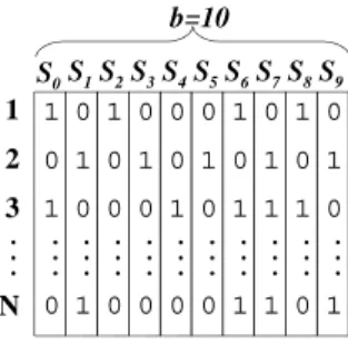
bit-slicing[9]. In this representation, there is a separate bit-slice vector stored individually for each bit of the signatures. When applying query q the bit slices where sig(q) has 1 are ANDed to derive a bit slice, representing the record-ids (rids) that pass the filter step (for containment and equality queries). Figure 1 shows an example of a bit-sliced signature file. If the query signature is 1001000100, we need to join slicesS0,S3, andS7in order to get the candidate rids. If the

partial join of some slices sets only a few rids, it might be beneficial not to retrieve and join the remaining slices, but to validateqdirectly on the qualifying rids. Overlap queries can be processed by taking the logical OR of the bit-vectors.

1 0 1

0 0 1 0

1 1 0 0

0 0 1 0

0 0 0 1

0 0 1 0

0 1 0 1

1 0 1 1

1 1 0 1

0 0 1 0

1 1

2 3

N

. . .

. . . b=10

S0S1S2S3S4S5S6S7S8S9

Figure 1: A bit-sliced signature file

The signature-tree [2, 10] is a hierarchical index, which clusters signatures based on their similarity. It is a dynamic, balanced tree, similar to the R–tree [6], where each node en-try is a tuple of the form _hsig, ptr_i. In a leaf node entry

sig is the signature andptr is the record-id of the indexed tuple. The signature of a directory node entry is the logi-cal OR of the signatures in the node pointed by it andptr

is a pointer to that node. In order to process a contain-ment/equality query we start from the root and follow the entry pointerse.ptr, if sig(q) _⊆e.sig, until the leaf nodes where qualifying signatures are found. For overlap queries all entries which intersect with sig(q) have to be followed. This index is efficient when there are high correlations be-tween the data signatures. In this case, the signatures at the directory nodes are sparse enough to facilitate search. On the other hand, if the signatures are random and

(3)

uncorre-lated the number of 1’s in the directory node entries is high and search performance degrades. A strength of the index is that it handles updates very efficiently, thus it is especially suitable for highly dynamic environments.

Another method for indexing signatures is based on hash-ing [8]. Given a smallk, the firstk bits are used as hash-keys and the signatures are split into 2k _{partitions. The} firstkbits of the query are then used to select the buckets which may contain qualifying results. To facilitate locating the qualifying buckets, a directory structure which contains hash values and pointers is stored separately (even in mem-ory if the number of buckets is small enough). In order to control the size of the directory and partitions dynamically, extendible hashing can be used. This index is very efficient for equality selection queries, since only one bucket has to be read for each query. The effect is the same as if we sorted the signatures and imposed a B+_{–tree over them, using a}

signature prefix as key. However, the performance of this index is not good for set containment queries [8].

2.2 The Inverted File

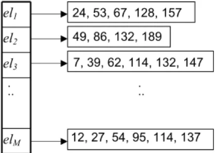
The inverted file is an alternative index for set-valued at-tributes. For each set element elin the domain D, an in-verted list is created with the record ids of the sets that contain this element in sorted order. Then these lists are stored sequentially on disk and a directory is created on top of the inverted file, pointing for each element to the offset of its inverted list in the file. If the domain cardinality|D|

is large, the directory may not fit in memory, so its entries

hel, of f setiare organized in a B+_{–tree having}_el_{as key.}

Given a query set q, assume that we want to find all sets that contain it. Searching on the inverted file is per-formed by fetching the inverted lists for all elements in q

and merge-joining them. The final list contains the record-ids of the results. For example, if the set containment query

q=_{el2, el3}is applied on the inverted file of Figure 2, only

tuple with rid=132 qualifies. Since the record-ids are sorted in the lists, the join is performed fast. If the search predi-cate is ‘overlap’, then the lists are just merged, eliminating duplicates. Notice that the inverted file can also process

-overlap queries efficiently since we just need to count the number of occurrences of each record-id in the merged list.

7, 39, 62, 114, 132, 147 24, 53, 67, 128, 157 49, 86, 132, 189

12, 27, 54, 95, 114, 137

el1

el2

. .. .

.. el3

elM

Figure 2: An inverted file

Fetching the inverted lists can incur many random ac-cesses. In order to reduce the access cost, the elements of

q are first sorted and the lists are retrieved in this order. Prefetching can be used to avoid random accesses if two lists are close to each other.

Updates on the inverted file are expensive. When a new

set is inserted, a number of lists equal to its cardinality have to be updated. An update-friendly version of the index al-lows some space at the end of each list for potential inser-tions and/or distributes the lists to buckets, so that new disk pages can be allocated at the end of each bucket. The in-verted file shares some features with the bit-sliced signature file. Both structures merge a set of rid-lists (represented in a different way) and are mostly suitable for static data with batch updates.

In recent comparison studies [15, 8], the inverted file was proven significantly faster than signature-based indexes, for set containment queries. There are several reasons for this. First, it is especially suitable for real-life applications where the sets are sparse and the domain cardinality large. In this case, signature-based methods generate many false drops. Second, it applies exact indexing, as opposed to signature-based methods, which retrieve a superset of the qualifying rids and require a refinement step. Finally, as discussed in the next subsection, it achieves higher compression rates, than signature-based approaches and its performance is less sensitive to the decompression overhead.

2.3 Compression

Both signature-based indexes and inverted files can use com-pression to reduce the storage and retrieval costs. Dense sig-natures are already compressed representations of sets, but sparse ones could require more storage than the sets (e.g., the exact signature representations of small sets). Thus, a way to compress the signatures is to reduce their length b

at the cost of increasing the false drop probability. Another method is to store the element-ids instead of the signature for small sets or to encode the gaps between the 1’s instead of storing the actual bitmap. However, this technique in-creases the cost of query processing; the signature has to be constructed on-the-fly if we want to still use fast bitwise operations. The bit-sliced index can also be compressed by encoding the gaps between the 1’s, but again this comes at the expense of extra query processing cost [15].

The compression of the inverted file is much more effec-tive. An inverted list is already sorted and can be easily compressed by encoding the gaps (i.e., differences) between consecutive rids. For example, assume that an inverted list contains the following rids: {11,24,57,102,145,173, ...}. It can be converted to the run-length encoding of the rids:

{11,13,33,45,43,28, ...}, i.e., the series of differences be-tween successive rids [16]. Observe that this comes at no cost for query processing, since the algorithm for merging the lists can be easily adapted. Although the above list con-tains small numbers there is no upper bound for them; a fixed-length encoding would yield no compression. Thus a variable-length encoding should be used.

An example of such an encoding is the Golomb coding [4]. Assume that the integers we want to encode follow a geometric law with a probability parameterp. The Golomb code takes a parametergsuch that (1−p)g+ (1−p)g+1≤

1 < (1−p)g−1+ (1−p)g. Now assume that we want to encode an integer x, wherex > 1. In order to save code space, we encodex−1 which is potentially 0. We represent (x−1) using two integers: l=b(x−1)/gcandr= (x−1) modulog. Finally,xis encoded using a unary encoding for

l+ 1 followed by a binary encoding of r. Table 1 shows the run-length integers in our running example and their Golomb codes for g = 16. For example, to compute the

(4)

code of 45 we derivel=_b(44/16)_c= 2 and r= 44 modulo 16 = 12, and concatenate the unary 3 = 110 with the binary 12 = 1100. Additional coding techniques are also applicable. See [16, 15] for more details on compressing inverted files.

number code

11 01011 13 01101 33 1100000 45 1101100 43 1101010 28 101011

Table 1: Example of Golomb codes for integers

Decoding the rids is quite fast and affects little the perfor-mance of the inverted file. Moreover, the compression rate increases with the density of the list, as the gaps between the rids decrease. To exemplify this, consider a relationR

of 100,000 tuples, where each setR.rhas 20 elements on the average, and the set domainD has 10,000 elements. The number of rids per inverted list is|R|×|R.r|_|D| = 200 on the av-erage. This means that the expected difference between two rids in an inverted list is_|R_|/200 = 500. If we use Golomb coding withg= 128 we can encode each rid with 10-11 bits on the average. Now assume that each set has 200 elements on the average. In this case, the expected difference between two rids is just 50 and we need fewer bits to encode them. Thus the size (and retrieval cost) of the inverted file increases sub-linearly with the average set cardinality. Moreover, the Golomb coding can be applied independently for each in-verted list adjusting the compression rate according to the data skew. The two extreme cases are lists containing few uncompressed integers, and lists which reduce to bitmaps.

3. Evaluation of Set Containment Joins

Several join operators can be applied on set-valued attributes, including the set containment, the set equality and the set overlap join. In this section we restrict our attention to the set containment join, which is one of the most interesting operators and also has been proven rather hard in past re-search [7, 13]. We first describe existing signature-based join algorithms. Then we propose and discuss the optimization of new algorithms that utilize inverted files. Throughout this section we will deal with the join R ₁r⊆s S, where r andsare set-valued attributes of relationsRandS, respec-tively. Unless otherwise specified, we will assume that none of the relations is indexed.

3.1 The Signature Nested Loops Join

In [7] two main memory join algorithms were proposed for the set containment join. One of them is also applicable for large relations that do not fit in memory. The Signature Nested Loops (SNL) Join consists of three phases. During the signature construction phase, for each tuple tS ∈ S a triplet_h|tS.s|, sig(tS.s), tS.ridiis computed, where |tS.s|is the cardinality oftS.s,sig(tS.s) is its signature, andtS.rid is the record-id oftS. These triplets are stored in a signature fileSsig. During theprobephase, each tupletR∈Ris read, its signature sig(tR.r) is computed and the signature file

Ssig is scanned to find all pairs htR.rid, tS.ridi, such that

sig(tR.r)⊆sig(tS.s) and|tR.r| ≤ |tS.s|. These rid-pairs are

written to a temporary relation. During the finalverification

phase the htR.rid, tS.ridi pairs generated from the probe phase are read, the corresponding tuples are fetched, and

tR.r⊆tS.sis verified.

This method requires a quadratic number (to the relation size) of signature comparisons and is not attractive for large problems. Notice that the verification phase could be com-bined with the match phase if we fetchtS.simmediately af-ter the signature comparison succeeds, however, this would incur many random accesses. In [7] a hash-based method is also proposed, however, it would result in a large number of random I/Os if applied to secondary memory problems.

3.2 The Partitioned Set Join

Ramasamy et al. [13] introduced a hash-based algorithm that aims at reducing the quadratic cost of SNL. The Par-titioned Set Join(PSJ) hashes the tuples fromRandS to a number ofP bucketsR1, R2, . . . , RP andS1, S2, . . . , SP and joinsRx withSx for all 1≤x≤P.

The algorithm also works in three phases. During the first (partitioning) phase, the tuples from the two relations are partitioned. Each tupletR ∈Ris read, and the triplet

h|tR.r|, sig(tR.r), tR.ridiis computed. Arandomelementer fromtR.r is picked and the triplet is written to the bucket determined by a hash function h(er). Then relation S is partitioned as follows. Each tuple tS ∈S is read, and the triplet h|tS.s|, sig(tS.s), tS.ridi is computed. For each ele-ment es intS.s, the triplet is written to the partition de-termined by the same hash functionh(es). If two elements

es∈tS.shave the same hash value the triplet is sent to the corresponding bucket only once. Thus, each triplet fromR

is hashed to exactly one partition, but a triplet fromS is in general hashed to many partitions. The algorithm does not miss join results, because if tR.r ⊆ tS.s then the random elementer∈tR.rwill equal somees∈tS.s, and the triplets will co-exist in the partition determined byh(er).

During thejoinphase, the pairs of partitionshRx, Sxi cor-responding to the same hash valuexare loaded and joined.

Rxshould be small enough to fit in memory; its contents are loaded and hashed using a secondary hash function. More specifically, a random set bit in eachsig(tR.r)∈Rxis picked and the triplet is assigned to the corresponding memory bucket. Then each triplet from Sx is compared with all triplets in the memory buckets determined by the set bits in

sig(tS.s). Qualifying rid-pairs are written to a temporary file. Finally, the verification phase of PSJ is the same as that of SNL.

Although PSJ is faster than SNL, if suffers from certain drawbacks. First, the replication of the signatures from S

can be high if the set cardinality is in the same order as the number of partitions P. Thus ifcis the cardinality of a tS.s ∈ S, the tuple will be hashed into c−c(1−1/c)P partitions on the average [7, 13]. For example if P = 100 and c = 50, the quantity above shows that each tuple is replicated to 43.3 partitions on the average. Thus the size of eachSxis comparable toSsigand the algorithm has sim-ilar cost to SNL (actually to a version of SNL that employs in-memory hashing; called PSJ-1 in [13]). On the other hand,P should be large enough in order to partitionRinto buckets that fit in memory. Second, PSJ carries the in-herent drawback of signature-based evaluation methods; it introduces false drops, which have to be verified. The verifi-cation phase incurs additional I/O and computational

(5)

over-head which constitutes a significant portion of the overall join cost, as shown in [13] and validated by our experiments. In the rest of this section we introduce join algorithms based on inverted files that alleviate these problems.

3.3 Block Nested Loops Using an Inverted File

As shown in [15], inverted files are more efficient than signa-ture-based indexes for evaluating selection queries. Among their other advantages once compression is taken into ac-count, it is mentioned that they are also relatively cheap to create.

This motivated us to study alternative methods for the set containment join, based on inverted files. Even if the relations are not indexed, it could be more beneficial to build inverted files and perform the join using them, rather than applying signature-based join techniques. Hopefully, this would yield two advantages. First, the join will be processed fast. Second, we would have built a powerful index that can be used afterwards not only for other join queries, but also for selections on the set-valued attribute, as described in Section 2. We will now discuss how to build inverted files fast and use them for evaluating set containment joins.

3.3.1 Constructing an inverted file

The inverted file for a relationR can be constructed fast using sorting and hashing techniques [12]. A simple method is to read each tupletR∈Rand decompose it to a number of binaryhel, tR.ridituples, one for each element-idelthat appears in the settR.r. Then these tuples are sorted on el and the index is built. For small relations this is fast enough, however, for larger relations we have to consider techniques that save I/O and computational cost. A better method is to partition the binary tuples using a hash function on el

and build a part of the index for each partition individu-ally. Then the indexes are concatenated and the same hash function is used to define an order for the elements.

In order to minimize the size of the partitions, before we write the partial lists of the partitions to disk, we can sort them ontR.ridand compress them. This comes at the ad-ditional cost of decompressing them and sort the tuples on

elto create the inverted lists for the partition. An alterna-tive method is to sort the partial lists onelin order to save computations when sorting the whole partition in memory. The cost of building the inverted file comprises the cost of reading the relations, the cost of writing and reading the partitions and the cost of writing the final inverted file. As we demonstrate in Section 5, if compression is used, the over-all cost is not much larger than the cost of readingR. This is due to the fact that the compressed partial information is several times smaller than the actual data.

3.3.2 A simple indexed nested-loops join method

The simplest and most intuitive method to perform the set containment join using inverted files is to build an inverted fileSIF forS and apply a set containment query for each tuple inR. It is not hard to see that ifSIF fits in memory, this method has optimal I/O cost.

However, for large problems SIF may not fit in memory and in the worst case it has to be read once for each tuple inR. Therefore, we should consider alternative techniques that apply in the general case.

3.3.3 Block Nested Loops Join

Since it is not efficient to scan the inverted file for each tuple from Rwe came up with the idea of splitting the inverted file in large blocks that fit in memory and scanR for each block. OurBlock Nested Loops(BNL) algorithm readsSIF sequentially in blocksB1, B2, . . . , BN, such that each block fits in memory and there is enough space for loading a page fromR. Assume that currently blockBiis loaded in mem-ory, and letLi be the set of elements whose inverted list is inBi. For each tupletR∈R, three cases may apply:

1. tR.r⊆Li; the lists of all elements intR.rare inBi. In this case the lists are joined and the qualifying results are output.

2. tR.r∩Li=∅; the list of no element intR.ris inBi. In this casetRis ignored and we go to the next tuple. 3. tR.r∩Li6=∅∧tR.r*Li; the lists of some (but not all) elements intR.rare inBi. This is the hardest case to handle, since we may need information from other blocks in order to verify whethertR has any superset inS. We calltR adanglingtuple.

The first two cases are trivial; thus we concentrate on han-dling dangling tuples efficiently. A simple way to manage a dangling tuple tR is to merge the lists intR.r∩Li (these are currently in memory), compute apartial rid list, and, if non-empty, write it to a temporary fileTi. The partial lists are of the formhtR.rid, n, tS1.rid, tS2.rid, . . . tSn.ridi, where

nis the number of tuples fromS that currently match with

tR.rid. If n is large, the list is compressed to save space. After we have scanned SIF, a second phase begins, which loads the temporary files and merge-joins them. The con-tents of eachTiare already sorted ontR.rid, thus merging them in memory is very efficient.

Figure 3 shows the pseudocode of BNL. lel denotes the inverted list of element el. In the implementation, Li is not computed explicitly, but the numbermof elementsel∈ tR.r∧lel∈Biis used to validate whethertR.r⊆Li; if|tR.r| equals m we know that all elements of tR.r are inLi. As a final comment, we assume that the directory for each Bi can fit in memory, since it should be much smaller than the block itself. We further compress it, by storing the offsets of each inverted list, with respect to the absolute offset of the first list inBi.

3.3.4 Optimizing BNL

The partial lists are many if the memory blocksBi are not large, and so is the overhead of writing (and reading) tem-porary results to disk. Therefore we have to minimize this temporary information at no additional cost in the join pro-cess.

3.3.4.1 KeepingπS.|s|in memory.

A fact that we have not exploited yet, is that a tupletR∈R could join with a tupletS∈S only if the cardinalities of the sets qualify _|tR.r| ≤ |tS.s|. If we use this information, we could shrink or prune many partial lists. The basic version of the inverted file does not include any information about

|tS.s|. We can obtain this information in two ways. The first is to store|tS.s|with every appearance oftS.ridin the inverted lists. This method is also used in [8]. However, the size of the inverted file may increase dramatically (it may

(6)

AlgorithmBN L(R,SIF){

i:= 0;

whilethere are more lists inSIF {

i:=i+ 1;

Bi:= read next block ofSIF that fits in memory;

Li:= elements whose inverted list is inBi; Initialize temporary fileTi;

foreach tupletR∈Rdo{

list(tR) :=T_l

el,el∈tR.r∧el∈Li;

iflist(tR)6=∅then

iftR.r⊆Li thenoutput results; elsewritelist(tR) toTi;

} } n:=i;

merge-join allTi, 1≤i≤nand output results;

}

Figure 3: Block-Nested Loops join

even double). In a compressed inverted file, we only need few bits (e.g., 10) to encode eachtS.rid, and storing|tS.s|could require that many extra bits. On the other hand, we observe that in typical applications, where sets are small,_|tS.s|does not require more than a byte to store. Thus we can keep the cardinalities of alltS.s∈S in memory (we denote this table byπ_S.|s|) without significant overhead. For example, if|S|=1M tuples, we need just a megabyte of memory to ac-commodateπS.|s|. This information can be computed and stored in memory while readingSat the construction phase ofSIF. It is then used to (i) accelerate the merging of in-verted lists, (ii) reduce the number and length of the partial lists that have to be written to temporary files.

3.3.4.2 Pipelining the partial lists.

Even with the availability of πS.|s|, the partial lists could be many and long. If an object’s elements are spanned to multiple blocks, multiple lists may have to be written to the temporary files. To make things worse, an object which is pruned while joining block Bi with R, because its lists there have empty intersection, may qualify at a later block

Bj, i < j, although it should never be considered again. For example, assume that atR∈Rhas two elements inB1

and their inverted lists have empty intersection. This means that there is no set inScontaining both elements, and as a result no set inS joins withtR. WhenB2is loaded, we can

find some elements intRwith lists inB2, which should not

normally be processed, since we already know thatt does not join with any tuple fromS.

Another observation is that while processing B2, we can

merge the partial lists generated by it with the lists inT1,

i.e., the temporary file created by the previous pass. Thus during the iteration where we joinBi with R, we keep in memory (i) blockBi, (ii) one (the current page) from R, and (iii) one (the current) page fromTi−1. Since we scanR

sequentially and the lists inTi−1are sorted ontR.rid, we can merge efficiently the lists produced by the previous passes with the ones produced by the current one. This makes it easier also to discard alltRwhich disqualified at the previous steps; if there is any elementel∈tR.rwhose inverted listlel

was at a previousBj,j < iand there is no list inTi−1 for

tR.rid, then we know thattR has been pruned before and we can ignore it at the current and next blocks. Another way to avoid processing tuples which disqualified during a previous block-join is to maintain a memory-resident bitmap indicating the pruned tuples fromR.

The pseudocode of this version of BNL that employs pi-pelining is shown in Figure 4. At each step, the qualifying lists from the current blockB ∈SIF are merged with the temporary file Tprev from the previous step. To perform merging efficiently we run a pointer on Tprev showing the current list lp. This serves multiple purposes. First, each

tR ∈ R which disqualified in some previous step is easily spotted (condition at line 1). Indeed, if the inverted list of some element from tR has been loaded before (this can be easily checked using the order of the elements in tR.r) and

tR.riddoes not match the currentlp.tR.ridinTprev, then we know thattR.ridhas been pruned before, because otherwise there would be an entry for it inTprev. The second use of

lp is to join its contents with the lists in B. If the current

tR has elements in the current block and matches with the currentlp, the lists inB are joined withlp. If the resulting list is not empty, the results are either output, or written to the next temporary fileTnext, depending on whether there are elements intRyet to be seen at a next step (cf. line 4 in Figure 4). lpis updated after the corresponding tuplelp.tR is read fromR(conditions at lines 2 and 3).

AlgorithmBN L(R,SIF){

Tprev := NULL;

B := read next block ofSIF that fits in memory;

L:= elements whose inverted list is inB; Initialize temporary fileTnext;

lp:= get next list fromTprev; /*if applicable*/ foreach tupletR∈R do{

(1) ifsome el_∈tR.rwas in some previousB

andlp.tR.rid6=tR.ridthen

continue; /*prune this tuple*/

iftR.r∩L=∅then{

(2) iflp.tR.rid=tR.ridthen

lp:= get next list fromTprev; /*if applicable*/

continue; /*goto next tuple*/

}

list(tR) :=Tlel,el∈tR.r∧el∈Li; (3) iflp.tR.rid=tR.ridthen{

list(tR) :=list(tR)∩lp;

lp:= get next list fromTprev; /*if applicable*/

}

iflist(t)6=∅then

(4) ifall inv. lists fortR.rhave been seen so farthen output results;

elsewritelist(tR) toTnext;

}

Tprev :=Tnext;

} }

(7)

3.3.4.3 Optimizing the computational cost.

Another factor which requires optimization is the join al-gorithm that merges the inverted lists in memory. We ini-tially implemented a multiway merge join algorithm with a heap (i.e., priority queue). The algorithm scans all lists synchronously increasing all pointers if all rids match, or the smallest one if they do not. The current positions of all pointers were organized in the heap to facilitate fast update of the minimum pointer. However, we found that this ver-sion performed rather slow, whereas most of the joined lists had high selectivity or gave no results.

Therefore, we implemented another version that performs a binary join at a time and joins its results with the next list. We experienced great performance improvement with this version, since since many sets fromRwith large cardinality were pruned much faster.

3.3.5 Analysis of BNL

The cost of BNL heavily depends on the size ofSIF. Clearly, given a memory bufferM, the smallerSIF is, the fewer the number of passes onRrequired by the algorithm. Also the more the inverted lists in a block, the fewer the temporary partial lists generated by each pass. The number of bits to store a compressed inverted fileIthat uses Golomb coding is in the worst case (assuming each inverted list has the same number of rids) given by the following formula [15]:

bits(I) =cN(1.5 + log₂|D|

c ), (1)

whereNis the number of indexed tuples,cis the average set cardinality and|D|is the domain size of the set elements. The factor in the parentheses is the average number of bits required to encode a “gap” between two rids in an inverted list. We can use this formula to estimate the size ofSIF. The I/O cost of BNL can then be estimated as follows:

IOBN L=size(SIF) +size(R)

size(SIF) M

+ 2Xsize(Ti) (2)

The last component in Equation 2 is the cost of reading and writing the temporary resultsTifor each blockBi. As-suming that the simple version of BNL is applied (without pipelining), allTiwill be equal, each containing the partial lists for the dangling tuples inBi. Assuming that rids are uniformly distributed in the inverted list, the probability

P robdng(tR) of a tR ∈ R to become a dangling tuple can be derived by the probability that all elements oftR to be contained inLiand the probability that no element intRis part ofLi, or else:

P robdng(tR) = 1− |Li|

c

+ |D|−|Li| c

|D| c

(3)

Lican be estimated by size_M(SIF) since we assume that all lists have the same size. The number of dangling tuples can then be found by_|R_|P robdng(tR). Not all dangling tuples will be written toTi, since some of them are pruned. The expected number of qualifying dangling tuples, as well as the size of their partial lists can be derived by applying probabilistic counting, considering the expected lengths of the lists and other parameters. The analysis is rather long and complex, therefore we skip it from the paper.

As shown in Section 5, the size of the temporary results is small, especially for largec, where the chances to prune a tuple are maximized. Moreover, the pipelining heuristic decreases fast the temporary results from one iteration to the next. For our experimental instances, where M is not much smaller thanSIF (e.g.,M ≥SIF/10),Ti is typically a small fraction of SIF, thus the I/O cost of BNL reduces roughly to the cost of scanningRtimes the number of passes.

3.4 An algorithm that joins two inverted files

The set containment join can also be evaluated by joining the two inverted filesRIF andSIF. Although this may re-quire preprocessing both relations, at a non-negligible cost, the resulting inverted files may accelerate search, and at the same time compress the information from the original rela-tions.

The join algorithm traverses synchronously both inverted files. At each step, the inverted lists are merged to par-tial lists htR.rid, n, tS1.rid, tS2.rid, . . . tSn.ridi, where n is the number of tuples fromS that match so far withtR.rid. Each inverted list pair generates as many partial lists as the number of tuples in the list of RIF. After scanning many inverted list pairs, the number of generated partial lists exceeds the memory limits and the lists are merged. The merging process eliminates lists with empty intersec-tion and outputs results if the number of merged lists for a tuple tR is equal to |tR.r|. The rest of the merged lists are compressed and written to a temporary file. In the final phase, the temporary files are loaded and joined. We call this methodInverted File Join(IFJ).

IFJ can be optimized in several ways. First, the projec-tionπR.|r| can be held in memory, to avoid fetching|tR.r| for verification. Alternatively, this information could be em-bedded in the inverted file but, as discussed above, at the non-trivial space cost. Another, more critical optimization is to minimize the size of the temporary files. For this, we use similar techniques as those for the optimization of BNL. We keepπ_S.|s|in memory, and use it to prune fast rid pairs, where |tR.r| > |tS.s|. Another optimization is to use the pipelining technique. Before we output the partial lists, the previous temporary file Tprev is loaded and merged with them. This may prune many lists. In addition, if we know that tR.r has no elements in inverted lists not seen so far, we can immediately output the_htR.rid, tSi.ridipairs, since they qualify the join.

However, this comes at the cost of maintaining an addi-tional tableRcount, which counts the number of times each

tR.rid has been seen in the inverted lists we have read so far from RIF. Since the sets are relatively sparse, we will typically need one character per tuple to encode this infor-mation. In other words, the size of this array is at most the size of πR.|r| and can be typically maintained in

mem-ory. Rcount is initialized with 0s. Whenever we read an

inverted list l inRIF we add 1 for each tR.rid present in

l. After a partial list has been finalized, we output the results if Rcount[tR.rid] = |tR.r|, otherwise we write the list to the temporary file. An additional optimization uses the equivalent table Scount for S, which can be used to prune some tSi.rid from the partial lists, as follows. If

|tR.r|−Rcount[tR.rid]>|tSi.s|−Scount[tSi.rid] we can prune

tSi.rid because in future lists the occurrences oftR.ridare more than the occurrences oftSi.rid. In other words, the elements of tR.r we have not seen yet are more than the

(8)

elements oftSi.swe have not seen yet, thustR.r*tSi.s.

4. Evaluation of Other Join Predicates

In this section we discuss the evaluation of other join oper-ators on set-valued attributes, namely the set equality join and the set overlap join.

4.1 The Set Equality Join

Adaptations of the signature-based and inverted-file based algorithms discussed in Section 3 can also be applied for the set equality join, since it is not hard to see that it is a special case of the set containment join.

From signature-based techniques, we do not consider SNL, since this algorithm compares a quadratic number of signa-tures and we can do much better for joins with high selec-tivity. PSJ on the other hand can be very useful for set equality queries. We propose an adapted version of PSJ for set equality joins. The main difference from the algorithm described in Section 3.2 is that we use a single method to partition the data for both relations. While computing the signature of each tuple intR ∈R we also find thesmallest element er ∈ tR.r (according to a predefined order in the domainD) and send the tripleth|tR.r|, sig(tR.r), tR.ridito the partition determined by a hash functionh(er). Tuples fromSare also partitioned in the same way. The rationale is that if two sets are equal, then their smallest elements should also be the same.

The join phase is also similar; each pair of partitions is loaded in memory and the contents are re-hashed in memory using a prefix of their signature (e.g., the first byte). Then all pairs of memory buckets (one pair for each value of the prefix) are joined by applying a signature equality test. The set cardinality is also used before the signature comparison to prune early disqualifying signature pairs. We expect that this version of PSJ will do much better than the one for set containment joins, since replication is avoided in both partitioning and join phases.

The inverted file algorithms BNL and IFJ, can also be adapted to process set equality joins. The only change in BNL is that πS.|s| is now used to prune fast inverted list rids of different cardinality than the current tR ∈ R. In other words, the condition_|tR.r| ≤ |tS.s|is now replaced by

|tR.r|=|tS.s|for each|tS.rid|found in the lists ofBi. IFJ is also changed accordingly (using bothπS.|s| andπR.|s|).

4.2 The Set Overlap Join

The set overlap join retrieves the pairs of tuples which have at least one common element. For the more general-overlap join, the qualifying pairs should share at least elements. In this paragraph we describe how these operators can be processed by signature-based methods and ones that use in-verted files.

The relaxed nature of the overlap predicate makes inap-propriate the application of hashing techniques, like PSJ, on signature representations. Indeed it is hard to define a par-titioning scheme which will divide the problem into joining

P pairs of buckets much smaller thanRandS. An idea we quickly abandoned is to partition bothRandS by replicat-ing their signatures to many hash buckets, after applyreplicat-ing a hash function on each of their elements. This approach does not miss any solution, but the size of partitions becomes so large that the overall cost becomes higher than apply-ing nested loops on two signature files. Another problem

with this partitioning approach is that it introduces dupli-cate drops. Thus, for this operator we use the simple SNL algorithm. Finally, notice that whatever signature-based method we use, the filtering step will be the same for all

-overlap queries independent to the value of, as discussed in Section 2.

On the other hand, algorithms that use inverted files could process overlap joins more efficiently. We propose an adap-tation of BNL as follows. At each pass BNL merges the inverted lists found inBifor eachtR. During merging, the number of occurrences for each tS.rid is counted. If this number is larger or equal to the threshold(i.e., we already found a matching pair of rids), the pair htR.rid, tS.ridi is written to a temporary fileQi. The remainder of the list is written to a fileTi, as before. Notice that if= 1, there will be no temporary files Ti. In this special case we also com-press the temporaryQi’s, since eachtRjoins with numerous

tS. After processing all blocks, BNL merges allTi’s to pro-duce a last file Qi+1 of qualifying results. The final phase

scans allQi’s (including the last one) and merges them to eliminate duplicates. Notice that each multiway merge is performed with a single scan over the temporary lists or re-sults, since these are produced sorted. This version of BNL is described in Figure 5. We comment only on the marked line (1), which avoids writing a partial list to Ti if all ele-ments oftRare in the current block. IftR.r⊆Li,tRcannot produce more qualifying pairs, since no more lists fortRwill be (or have been) produced.

AlgorithmBN L(R,SIF,){

i:= 0;

i:=i+ 1;

Bi := read next block ofSIF that fits in memory;

Li := elements whose inverted list is inBi; Initialize temporary fileTi;

Initialize temporary fileQi; foreach tupletR∈R do{

list(tR) :=Slel,el∈tR.r∧el∈Li;

foreachtS.ridinlist(tR)do

iftS.ridappears at leasttimesthen{ remove alltS.ridfromlist(tR); append_htR.rid, tS.riditoQi;} (1) iflist(tR)6=∅andtR.r*Lithen

writelist(tR) toTi;

} } n:=i;

merge allTi, 1≤i≤nto produceQi+1;

merge allQi, 1≤i≤n+ 1 to eliminate duplicates;

}

Figure 5: Block-Nested Loops (set overlap)

IFJ can also be adapted the same way as BNL for overlap joins. A set of temporary files and result files Ti and Qi are produced as the algorithm merges the inverted lists. A special feature of IFJ is that, for = 1 and if we ignore duplicate elimination, it can output results immediately and at the minimal cost of reading the inverted files.

(9)

5. Experiments

In this section we evaluate the performance of join algo-rithms on set-valued attributes. We first compare the pro-posed algorithms for set containment joins with PSJ, the previously proposed signature-based method. Afterwards, we evaluate the performance of signature-based and inverted file methods for other join predicates. The experiments were performed on a PC with a Pentium III 800MHz processor and 256MB of memory, running Linux 2.4.7-10. In the next subsection we describe the generator we used for our test data.

5.1 Data Generation

We generated synthetic relations with set-valued data us-ing the same generator as in [13]. The parameters of the generator are the relation cardinality, the average set car-dinality in a tuple, the domain size of set elements, and a correlation percentagecorr. The domain of size|D|is rep-resented by the set of first_|D_|integers for simplicity, and without loss of generality (such a mapping is typically used in real applications to reduce the space requirements of the tuples and the comparison costs). The domain is split into 50 equal-sized subdomains. Elements which fall in the same subdomain, model elements falling in the same real-world class (i.e., correlated elements).

The correlation percentage is used to tune the number of elements in a set which are correlated (i.e., fall in the same class). Thus, the relation is generated as follows. For each tuple, we pick a class according to a distribution (unless otherwise stated, we consider a uniform distribution). Then

corr% of the set elements are picked from this sub-domain and the rest of them are randomly chosen from the remain-ing 49 subdomains. For set containment joins the data were generated, such that the size of the join result was controlled to be in the order of_|R_|. Finally, in all experiments, unless otherwise stated,RandS were generated to have the same cardinality, the correlation is set to 10%, and|D|=10,000. The same settings are used in the experiments of [13].

5.2 Set Containment Joins

In this subsection, we compare the performance of three algorithms for set containment joins. The first is the state-of-the-art PSJ algorithm proposed in [13]. The other two are BNL (described in Section 3.3) and IFJ (described in Section 3.4). We do not consider SNL, since it is inferior to PSJ, as shown in [13]. Unless otherwise specified, we used all optimization techniques for our proposed algorithms, (i.e., keeping the set cardinality projections in memory, pipelin-ing, pairwise join implementation). For fairness to PSJ, in the overall cost we included the construction of the inverted files, wherever applicable.

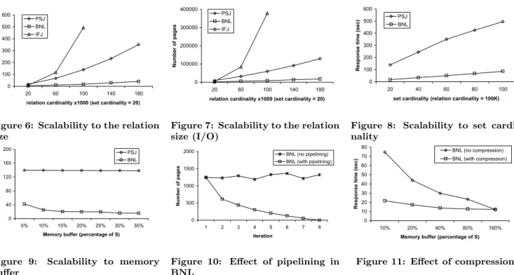
In the first experiment, we compare the performance of the three methods for the following setting: |R|=|S|, the average set cardinalitycis set to 20, the relation cardinality ranges from 20K to 180K and the memory buffer is set to 15% of the size ofS on disk. Figure 6 shows the cost of the three methods for various relation cardinalities.

BNL is clearly the winner. The other algorithms suffer from the drawbacks discussed in Section 3. In terms of scalability, BNL is also the best algorithm; its cost is sub-quadratic to the problem size. This is due to the fact that even with only a small memory buffer,SIF is split to a few blocks andRis scanned only a few times. In our

experimen-tal settings and for all instances of Figure 6, the number of blocks was just 2. On the other hand, both PSJ and IFJ do not scale well with the problem size. IFJ, in specific, produces a huge number of intermediate results, once the number of rids in the inverted lists increase. This is some-how expected, because IFJ generates a quadratic number of candidate rid pairs for each pair of inverted lists it joins.

Figure 7 shows the number of pages accessed by each al-gorithm. The page size is set to 4K in all experiments. The figure indicates that the I/O cost is the dominant factor for all algorithms, especially for IFJ, which generates a large number of temporary lists. The majority of the page ac-cesses are sequential, thus the I/O cost translates mainly to disk transfer costs.

Figure 12 shows “where the time goes” in the experimen-tal instance |R|=|S|= 100K. Notice that the bar for IFJ has been truncated for better visualization. Starting from the bottom, each bar accumulates the I/O and computa-tional costs for partitioning (PSJ) or building the inverted files (BNL and IFJ), for joining (join phase of PSJ and over-all join costs of BNL and IFJ), and for verifying the candi-date rid-pairs (this applies only to PSJ). The burden of each algorithm can be easily spotted.

Sheet3

0 100 200 300 400 500 600

20 60 100 140 180

relation cardinality x1000 (set cardinality = 20)

R

esponse t

im

e (

sec)

PSJ BNL IFJ

0 20 40 60 80 100 120 140 160

PSJ BNL IFJ

CPU/IO cost breakdown (rel. card. = 100K, set card. = 20)

Response t

im

e

(

sec)

IO (verify) CPU (verify) IO (join) CPU (join) IO (part/IF) CPU (part/IF)

0 100 200 300 400 500 600

20 40 60 80 100

set cardinality (relation cardinality = 100K)

R

esponse t

im

e (

sec)

PSJ BNL

Page 1

Figure 12: Cost breakdown (set containment)

The cost of PSJ is split evenly in all three phases. The algorithm generates a large number of replicated triplets for each tS ∈ S. The triplets have to be written to the tem-porary files, re-read and joined with the partitions of R. Thus, PSJ spends a lot of time in partitioning (much more than the time needed to construct an inverted file). The join phase of PSJ is also slow, requiring many computations to derive the candidate pairs. Finally, the verification cost is also high due to the large number of false drops. Notice that the parameters of PSJ have been tuned according to the analysis in [13] and they are optimal for each experi-mental instance. For example, if we increase the signature length the I/O cost of partitioning and joining the data in-creases at the same rate, but the number of candidates and the verification cost drop. On the other hand, decreasing the signature length leads to smaller partitions but explodes the number of candidate rid-pairs to be verified.

The burden of IFS is the I/O cost of writing and reading back the temporary lists. The algorithm is less systematic than BNL, since it generates at a huge number of lists at a time, which cannot be managed efficiently. Apart from this, its computational cost is also high (mainly due to sorting a

(10)

Sheet3 0 100 200 300 400 500 600

20 60 100 140 180

R esponse t im e ( sec) PSJ BNL IFJ 0 20 40 60 80 100 120 140 160

PSJ BNL IFJ

Response t im e ( sec) IO (verify) CPU (verify) IO (join) CPU (join) IO (part/IF) CPU (part/IF) 0 100 200 300 400 500 600

20 40 60 80 100

R esponse t im e ( sec) PSJ BNL Page 1

Figure 6: Scalability to the relation size Sheet3 0 100000 200000 300000 400000

20 60 100 140 180

N u m b er of pages PSJ BNL IFJ 0 40 80 120 160 200

5% 10% 15% 20% 25% 30% 35%

Memory buffer (percentage of S)

R esponse t im e ( sec) PSJ BNL 0 1000 2000 3000 4000

1 2 3 4 5 6 7 8

iteration N u m b er of pages

BNL (no pipelining) BNL (with pipelining)

Page 3

Figure 7: Scalability to the relation size (I/O) Sheet3 0 100 200 300 400 500 600

20 60 100 140 180

R esponse t im e ( sec) PSJ BNL IFJ 0 20 40 60 80 100 120 140 160

PSJ BNL IFJ

Response t im e ( sec) IO (verify) CPU (verify) IO (join) CPU (join) IO (part/IF) CPU (part/IF) 0 100 200 300 400 500 600

20 40 60 80 100

R esponse t im e ( sec) PSJ BNL Page 1

Figure 8: Scalability to set cardi-nality Sheet3 0 100000 200000 300000 400000

20 60 100 140 180

5% 10% 15% 20% 25% 30% 35%

1 2 3 4 5 6 7 8

Page 3

Figure 9: Scalability to memory

buffer All 0 100000 200000 300000 400000

20 60 100 140 180

5% 10% 15% 20% 25% 30% 35% Memory buffer (percentage of S)

1 2 3 4 5 6 7 8

Page 3

Figure 10: Effect of pipelining in BNL Sheet3 0 10 20 30 40 50 60 70 80

10% 20% 40% 80% 160%

Response t

im

e

(

sec)

BNL (no compression) BNL (with compression)

Page 2

Figure 11: Effect of compression

large number of lists prior to merging them), indicating that this method is clearly inappropriate for the set containment join. Thus, we omit it from the remainder of the evaluation. On the other hand, BNL processes set containment joins very fast. Notice thatSIF is constructed quite fast, due to the employment of the compression techniques. The join phase is slightly more expensive that the inverted file con-struction. In this experimental instance,Ris scanned twice, dominating the overall cost of the algorithm, since the gen-erated temporary results andSIF are small (SIF is just 28% ofS), compared to the size of the relation.

The next experiment (Figure 8) compares PSJ with BNL for_|R_|=_|S_|= 100K and various values of the average set cardinalityc. The performance gap between the two meth-ods is maintained with the increase ofc; their response time increases almost linearly withc. This is expected for BNL, since the lengths of the inverted lists are proportional to

c. The I/O cost of the algorithm (not shown) increases with a small sublinear factor, due to the highest compression achieved. PSJ also hides a small sublinear factor, since the ratio of false drops decreases slightly with the increase ofc. Finally, we have to mention that the cost of IFJ (not shown in the diagram) explodes with the increase ofc, because of the quadratic increase of the produced rid-lists; the higher

|tR.r|is, the larger the number of inverted lists that contain

tR.rid, and the longer the expected time to visit all these lists in order to output the matching pairs for this tuple.

We also compared the algorithms under different condi-tions, (e.g.,_|R_{| 6}=_|S_|, different correlation values, etc.), ob-taining similar results. BNL is typically an order of mag-nitude faster than PSJ. Notice, however, that the efficiency of BNL depends on the available memory. In the next ex-periment, we validate the robustness of the algorithm for a range of memory buffer values. The settings for this and the remaining experiments in this section are _|R_| =_|S_| =

100K and c = 20. Figure 9 plots the performance of PSJ and BNL as a function of the available memory buffer. No-tice that even with a small amount of memory (case 5% is around 350Kb), BNL is significantly faster than PSJ. The algorithm converges fast to its optimal performance with the increase of memory. On the other hand, PSJ joins a large amount of independent partitioned information and exploits little the memory buffer.

The next experiment demonstrates the effectiveness of the pipelining heuristic in BNL. We ran again the previous ex-perimental instance for the case where the memory buffer is 5% the size ofS. The number of blocksSIF is divided to is 8 in this case. Figure 10 shows the number of intermediate results generated by BNL at each pass, compared to the re-sults generated by the basic version of BNL that does not use pipelining. The results are lists of variable size (some compressed, some not) and we measure them by the num-ber of pages they occupy on disk. Observe that pipelining reduces significantly the size of intermediate results as we proceed to subsequent iterations. Many lists are pruned in the latter passes, because (i) they are unsuccessfully merged with the ones from the previous pass, (ii) the corresponding tuple has already been pruned at a previous pass, or (iii) no more elements of the tuple are found in future lists and the current results are output. On the other hand, the basic ver-sion of BNL generates a significant amount of intermediate results, which are only processed at the final stage.

Finally, we demonstrate the effectiveness of compression in BNL. Figure 11 shows the performance of BNL and a version of the algorithm that does not use compression, as a function of the available memory. The effects of using compression are two. First, building the inverted file is now less expensive. Second, the number of inverted lists from

SIF that can be loaded in memory becomes significantly smaller. As a result, more passes are required, more

(11)

tempo-rary results are generated, and the algorithm becomes much slower. The performance of the two versions converges at the point where the uncompressedSIF fits in memory. A point also worth mentioning is that the version of BNL that does not use compression is faster than PSJ (compare Fig-ures 10 and 11) even for small memory buffers (e.g., 10% of the size ofS).

To conclude, BNL is a fast and robust algorithm for the set containment join. First, it utilizes compression for better memory management. Second, it avoids the extensive data replication of PSJ. Third, it exploits greedily the available memory. Fourth, it employs a pipelining technique to shrink the number of intermediate results. Finally, it avoids the expensive verification of drops required by signature-based algorithms.

5.3 Other Join Operators

In this section, we compare signature-based methods with inverted file methods for other join predicates. In the first experiment, we compare the performance of the three meth-ods evaluated in the previous section for set equality joins under the following setting:|R|=|S|, the average set cardi-nalitycis set to 20, the relation cardinality varies from 20K to 180K and the memory buffer is set to 15% of the size of

S on disk. Figure 13 shows the cost of the three methods for various relation cardinalities.

All

0 10 20 30 40 50 60 70 80

10% 20% 40% 80% 160%

Response t

im

e

(

sec)

0 10 20 30 40 50 60 70 80 90

20 60 100 140 180

R

esponse t

im

e (

sec)

PSJ BNL IFJ

Page 2

Figure 13: Varying _|R_| (set equality join)

Observe that PSJ and BNL perform similarly in all ex-perimental instances. They both manage to process the join fast for different reasons. PSJ avoids the extensive replica-tion (unlike in the set containment join). It also manages to join the signatures fast in memory, using the prefix hashing heuristic. On the other hand, it still has to verify a signifi-cant number of candidate object pairs. The verification cost of the algorithm sometimes exceeds the cost of partitioning and joining the signatures.

BNL is also fast. Its performance improves from the set containment join case, although not dramatically. Many partial lists and rids are pruned due to the cardinality check and the temporary results affect little the cost of the algo-rithm. The decrease of the join cost makes the index con-struction an important factor of the overall cost. Finally, IFJ performs bad for set equality joins, as well. The arbi-trary order of the generated lists and the ad-hoc nature of the algorithm make it less suitable for this join operation.

Figure 14 shows the performance of the algorithms, when the relation cardinality is fixed to 100K and the set

cardinal-ity varies. The conclusion is the same: PSJ and BNL have similar performance, whereas the cost of IFJ explodes with the set cardinality, because of the huge number of inverted lists that need to be merged.

All

0 10 20 30 40 50 60 70 80

10% 20% 40% 80% 160%

Response t

im

e

(

sec)

0 10 20 30 40 50 60 70 80 90

20 60 100 140 180

R

esponse t

im

e (

sec)

PSJ BNL IFJ

0 100 200 300 400

20 60 100 140 180

R

esponse t

im

e (

sec)

PSJ BNL IFJ

Page 2

Figure 14: Varying c(set equality join)

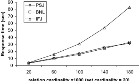
In the final experiment we compare SNL, BNL and IFJ for set overlap joins. Figure 15 shows the performance of the algorithms for _|R_|= _|S_|= 20K and c = 20. The ex-treme cost of the signature-based method makes it clearly inappropriate for set overlap joins. The selectivity of the signatures is low, even if a large signature length is picked, and the ratio of false drops is huge. In this setting, 86% of the pairs qualified the signature comparison, whereas only 4% are actual results for=1. Moreover, the increase of

(and the selectivity of the join) does not affect the signature selectivity (as discussed in Section 2). BNL is faster than IFJ, although it generates many temporary results. There are two reasons for this. First, some results are output im-mediately because we know that they cannot match with lists in other blocks. Second, IFJ spends a lot of time in sorting, due to the less systematic production of the tempo-rary lists. Notice that for= 1 the cost of BNL is higher than for other values ofdue to the higher overhead of the result size. On the other hand, IFJ is less sensitive than BNL to the value of.

All

1 10 100 1000 10000

1 2 3 4 5 set overlap join (|R| = 20K, c = 20)

R

esponse t

im

e (

sec)

SNL BNL IFJ

Page 4

Figure 15: Varying(set overlap join)

As an overall conclusion, BNL the most appropriate algo-rithm for set overlap joins, too. In the future, we plan to optimize further this algorithm for this join operator, and also study its adaptation to other related query types, like the set similarity join. Arguably, the present

(12)

implementa-tion is not output sensitive; although the query result size reduces significantly with, this is not reflected to the evalu-ation cost, due to the a large number of temporary lists. An optimization we have not studied yet is to consider which of

RandSshould be placed as the “outer” relation in equality and overlap joins, since these operators are symmetric (as opposed to the set containment join).

6. Conclusions

In this paper, we studied the efficient processing of various join predicates on set-valued attributes. Focusing on the set containment join, we introduced a new algorithm which creates an inverted file for the “container” relation S and uses it to find in a systematic way for each object in the “contained” relationR its supersets inS. This algorithm is a variation of block nested loops (BNL) that gracefully exploits the available memory and compression to produce fast the join results. BNL consistently outperforms a pre-viously proposed signature-based approach, typically by an order of magnitude. If the relations are already indexed by inverted files1, join processing can be even faster.

We also devised adaptations of signature-based and in-verted file methods for other two join operators; the set equality join and the set overlap join. The conclusion is that signature-based methods are only appropriate for set equality joins. For the other join types, a version of BNL is always the most suitable algorithm. On the other hand, a method that joins two inverted files was found inappropriate for all join types.

In the future, we plan to study additional, interesting set join operators. Theset similarity join, retrieves object pairs which exceed a given similarity threshold. This join type is very similar to the-overlap join, however, the similarity function is usually more complex, depending on both overlap and set cardinality. Another variation is the closest pairs

query [1], which retrieves from the Cartesian productR_×S

thekpairs with the highest similarity (or overlap). A similar operation is theall nearest neighborquery, which finds for each set in R its nearest neighbor in S. This query has been studied in [11], where inverted files were used, but the proposed algorithms were not optimized and only the I/O cost was considered for evaluating them.

Acknowledgements

This work was supported by grant HKU 7380/02E from Hong Kong RGC.

References

[1] A. Corral, Y. Manolopoulos, Y. Theodoridis, and M. Vassilakopoulos. Closest pair queries in spatial databases. InProc. of ACM SIGMOD Int’l Conference, 2000.

[2] U. Deppisch. S-tree: A dynamic balanced signature in-dex for office retrieval. In Proc. of ACM SIGIR Int’l Conference, 1986.

[3] C. Faloutsos. Signature files. InInformation Retrieval: Data Structures and Algorithms, pages 44–65, 1993. [4] S. W. Golomb. Run length encodings.IEEE

Transac-tions on Information Theory, 12(3):399–401, 1966.

1_{We expect this to be a typical case, in applications that}

index sets for containment queries [15, 8].

[5] R. H. G¨uting. An introduction to spatial database sys-tems.VLDB Journal, 3(4):357–399, 1994.

[6] A. Guttman. R-trees: a dynamical index structure for spatial searching. InProc. of ACM SIGMOD Int’l Con-ference, 1984.

[7] S. Helmer and G. Moerkotte. Evaluation of main mem-ory join algorithms for joins with set comparison join predicates. InProc. of VLDB Conference, 1997. [8] S. Helmer and G. Moerkotte. A study of four index

structures for set-valued attributes of low cardinality. InTechnical Report, University of Mannheim, number 2/99. University of Mannheim, 1999.

[9] Y. Ishikawa, H. Kitagawa, and N. Ohbo. Evaluation of signature files as set access facilities in oodbs. InProc. of ACM SIGMOD Int’l Conference, 1993.

[10] N. Mamoulis, D. W. Cheung, and W. Lian. Similar-ity search in sets and categorical data using the signa-ture tree. In Proc. of Int’l Conf. on Data Engineering (ICDE), 2003.

[11] W. Meng, C. T. Yu, W. Wang, and N. Rishe. Perfor-mance analysis of three text-join algorithms. TKDE, 10(3):477–492, 1998.

[12] A. Moffat and T. Bell. In-situ generation of compressed inverted files.Journal of the American Society of Infor-mation Science, 46(7):537–550, 1995.

[13] K. Ramasamy, J. M. Patel, J. F. Naughton, and R. Kaushik. Set containment joins: The good, the bad and the ugly. InProc. of VLDB Conference, 2000. [14] M. Stonebraker. Object-relational DBMS: The Next

Great Wave. Morgan Kaufmann, 1996.

[15] J. Zobel, A. Moffat, and K. Ramamohanarao. Inverted files versus signature files for text indexing. TODS, 23(4):453–490, 1998.

[16] J. Zobel, A. Moffat, and R. Sacks-Davis. An efficient indexing technique for full text databases. InProc. of VLDB Conference, 1992.

[17] J. Zobel, A. Moffat, and R. Sacks-Davis. Searching large lexicons for partially specified terms using compressed inverted files. InProc. of VLDB Conference, 1993.