Vol 8, No 3 (2017)

(1)

Available online throug

ISSN 2229 – 5046

HALL EFFECTS ON THE PERISTALTIC PUMPING

OF A HYPERBOLIC TANGENT FLUID IN A PLANAR CHANNEL

K. SUBBA NARASIMHUDU

1

**_{, M. V. SUBBA REDDY*}**

2

1

_{Research Scholar, Department of Mathematics,}

Rayalaseema University, Kurnool-518002, (A.P.), India.

2

_{Professor, Department of CSE,}

Sri Venkatesa Perumal College of Engineering & Technology, Puttur-517583, (A.P.), India.

(Received On: 23-02-17; Revised & Accepted On: 18-03-17)

ABSTRACT

I

n this paper, we investigated the effect of Hall on the peristaltic pumping of a hyperbolic tangent fluid in a planar channel under the assumption of long wavelength. The expressions for the velocity and axial pressure gradient are obtained by employing perturbation technique. The effects of Weissenberg number, power-law index, Hall parameter, Hartmann number and amplitude ratio on the axial pressure gradient, time-averaged volume flow rate and the friction force at the wall are analyzed with the help of graphs.

Keywords: Hyperbolic tangent fluid, power-law index, Hall parameter, Hartmann number peristaltic pumping.

1. INTRODUCTION

Extensive study of peristalsis has been carried out for a Newtonian with a periodic train of sinusoidal peristaltic waves. The inertia – free peristaltic trsnsport with long wavelength analysis was given by Shapiro et al. [14]. The early developments on the mathematical modeling and experimental fluid mechanics of peristaltic flow were given in a comprehensive review by Jaffrin and Shapiro [8]. However, the rheological properties of the fluids can affect these characteristics significantly. Moreover, most of the physiological fluids are known to be non-Newtonian. It is well known that some fluids which are encountered in chemical applications do not adhere to the classical Newtonian viscosity prescription and are accordingly known as non-Newtonian fluids. One especial class of fluids which are of considerable practical importance is that in which the viscosity depends on the shear stress or on the flow rate. The viscosity of most non-Newtonian fluids, such as polymers, is usually a nonlinear decreasing function of the generalized shear rate. This is known as shear-thinning behavior. Such fluid is a hyperbolic tangent fluid (Ai and Vafai [1]). Nadeem and Akram [11] have first investigated the peristaltic flow of a hyperbolic tangent fluid in an asymmetric channel. Nadeem and Akbar [10] have analyzed the peristaltic transport of a Tangent hyperbolic fluid in an endoscope

numerically. Akbar et al. [2] have discussed the

Based on Experimental controls, it was shown that the controlled application of low intensity and frequency pulsing magnetic fields could modify cell and tissue behavior. Biochemistry has taught us that cells are formed of positive or negative charged molecules. This is why these magnetic fields applied to living organisms may induce deep modifications in molecule orientation and in their interaction. An impulse magnetic field in the combined therapy of patients with stone fragments in the upper urinary tract was experimentally studied by Li et al. [9]. It was found that impulse magnetic field (IMF) activates impulse activity of ureteral smooth muscles in 100% of cases. Elshahed and Haroun [4] have investigated the peristaltic flow of a Johnson-Segalman fluid in a planar channel under the effect of a magnetic field. Hayat and Ali [6] have investigated the peristaltic motion of a MHD third grade fluid in a tube. Hayat

et al. [7] have first investigated the Hall effects on the peristaltic flow of a Maxwell fluid trough a porous medium in channel. Magnetohydrodynamic peristaltic flow of a hyperbolic tangent fluid in a vertical asymmetric channel with heat transfer was studied by Nadeem and Akram [12]. Prasanth Reddy and Subba Reddy [13] have analyzed the peristaltic pumping of third grade fluid in an asymmetric channel under the effect of magnetic fluid. Effect of variable viscosity on the peristaltic flow of a Jeffrey fluid in a tube under the effect of a magnetic field was investigated by Gangavathi et al. [5]. Recently Eldabe [3] have studied the Hall Effect on peristaltic flow of third order fluid in a porous medium with heat and mass transfer.

(2)

© 2017, IJMA. All Rights Reserved 71 Motivated by these, we investigated the effect of Hall on the peristaltic pumping of a hyperbolic tangent fluid in a planar channel under the assumption of long wavelength. The expressions for the velocity and axial pressure gradient are obtained by employing perturbation technique. The effects of Weissenberg number, power-law index, Hall parameter, Hartmann number and amplitude ratio on the axial pressure gradient, time-averaged volume flow rate and the friction force at the wall are analyzed with the help of graphs.

2. MATHEMATICAL FORMULATION

We consider the peristaltic motion of a hyperbolic tangent fluid in a two-dimensional symmetric channel of width 2a

under the effect of magnetic field. The flow is generated by sinusoidal wave trains propagating with constant speed

c

along the channel walls. A uniform magnetic field

0

B is applied in the transverse direction to the flow. The magnetic Reynolds number is considered small and so induces magnetic field neglected. Fig. 1 represents the physical model of the channel.

Figure-1: The Physical Model

The wall deformation is given by

2 ( , )

cos

(

)

Y

H X t

a

b

π

X

ct

λ

= ±

= ± ±

−

, (2.1)

where b is the amplitude of the wave,

λ

- the wave length and

X

and

Y

- the rectangular co-ordinates with

X

measured along the axis of the channel and

Y

perpendicular to

X

. Let

( , )

U V

be the velocity components in fixed

frame of reference

( , )

X Y

.

The flow is unsteady in the laboratory frame

( , )

X Y

. However, in a co-ordinate system moving with the propagation velocity c (wave frame (x, y)), the boundary shape is stationary. The transformation from fixed frame to wave frame is given by

,

x

=

X

−

ct y

=

Y u

= −

U

c v

=

V

(2.2)

where

( , )

u v

and

( , )

U V

are velocity components in the wave and laboratory frames respectively.

The constitutive equation for a Hyperbolic Tangent fluid is

(

0

)

tanh

( )

n

τ

= −



_

η

_∞

+

η η

+

_∞

Γ

γ





_

γ



(2.3)

where

τ

is the extra stress tensor,

η

_∞ is the infinite shear rate viscosity,

η

_o is the zero shear rate viscosity,

Γ

is the time constant,

n

is the power-law index and

γ



is defined as

1

2

i j ij ji

2 γ



=

∑∑

γ γ

 

=

π

(2.4)

where

π

is the second invariant stress tensor. We consider in the constitutive equation (2.3) the case for which

0 η

_∞

=

and

Γ <

γ



1

, so the Eq. (2.3) can be written as

( )

(

)

(

[

]

)

0 0

1

0

1

n n

n

(3)

The above model reduces to Newtonian for

Γ =

0

and

n

=

0

.

The equations governing the flow in the wave frame of reference are

0 u

v

x

y

∂

₊

∂

₌

∂

(2.6)

(

)

(

)

2 0 2

1

yx xx

B

u

p

u

v

mv

u

c

x

y

x

y

m

τ

σ

ρ



_

∂

+

∂



_

= −

∂

−

∂

−

∂

+

−

+

∂

+





(2.7)

(

)

(

)

2 0 2

1

xy yy

B

v

p

u

v

m u

c

v

x

y

x

y

m

τ

_σ

ρ



_

∂

+

∂



_

= −

∂

−

∂

−

∂

−

+ +

∂

+





(2.8)

where

ρ

is the density

σ

is the electrical conductivity,

B

₀ is the magnetic field strength and

m

is the Hall parameter.

The corresponding dimensional boundary conditions are

u

= −

c

at

y

=

H

(2.9)

0 u

y

∂

=

∂

at

y

=

0

(2.10)

Introducing the non-dimensional variables defined by

2

0

, ,

, , ,

,

x

y

u

v

a

pa

b

x

y

u

v

p

a

c

δ

c

φ

a

λ

δ

λ

η λ

=

0 0 0

, ,

xx _xx

,

_xy _xy

,

yy _yy

,

H

ct

a

h

t

a

c

λ

τ

λ

η

=

0

Re

ac

,

We

c

, ,

a

q

a

c

ac

ρ

_γ

γ

η

Γ

=



=



=

(2.11)

into the Equations (2.6) - (2.8), reduce to (after dropping the bars)

0 u

v

x

y

∂

₊

∂

₌

∂

(2.12)

(

)

2 2 2

Re

1

xy xx

u

p

M

u

v

u

x

y

x

y

m

τ

δ

_



∂

+

∂

_



= −

∂

−

δ

∂

−

∂

−

+

∂

+





(2.13)

(

)

(

)

2 3 2 2

Re

1

xy yy

v

p

M

u

v

m u

v

x

y

m

τ

δ



_

∂

+

∂

_



= −

∂

−

δ

∂

−

δ

∂

−

+ +

δ

∂

+





(2.14)

where _xx

2 1

n We

(

1 )

u

x

τ

= −  +

_

γ



− 

_{ ∂}

∂

, _xy

1 n We

(

1 )

u

2

v

y

x

τ

= −  +

_

γ

− 

_{ ∂}



_

∂

+

δ

∂



_

∂







,

(

)

2

1

yy

v

n We

y

τ

= −  +

δ

_

γ



− 

_{ ∂}

∂

,

1

2 2

2 2 2

2 u

u

v

2 v

x

y

x

y

γ

=





δ

_



∂



_

+

_



∂

+

δ

∂

_



+

δ



_

∂



_





∂























and 0 0

M

aB

σ

η

=

is the Hartmann number.

Under lubrication approach, neglecting the terms of order

δ

and Re, the Eqs. (2.13) and (2.14) become

(

)

2 2

1

1 p

u

M

n We

u

x

y

m













∂

₌

∂



₊

∂

₋

∂



₋

₊













(4)

0 p

y

∂

₌

∂

(2.16)

From Eq. (2.15) and (2.16), we get

(

1 )

2₂ 2 2₂

(

1 )

1 dp

u

M

n

nWe

u

dx

y

m



_

_



∂

=

−

+



_

_



−

+

∂

_

_

_

∂

_

_

_

+

(2.17)

The corresponding non-dimensional boundary conditions in the wave frame are given by

1 u

= −

at

y

= = +

h

1 φ

cos 2

π

x

(2.18)

0 u

y

∂

₌

∂

at

y

=

0

(2.19)

The volume flow rate

q

in a wave frame of reference is given by

0

h

q

=

∫

udy

. (2.20)

The instantaneous flow

Q X t

(

, )

in the laboratory frame is

0 0

(

, )

(

1)

h h

Q X t

=

∫

UdY

=

∫

u

+

dy

= +

q

h

(2.21)

The time averaged volume flow rate

Q

over one period

T

c

λ



₌











of the peristaltic wave is given by

0

1

T

Q

Qdt

q

T

=

∫

= +

(2.22)

3. SOLUTION

Since Eq. (2.17) is a non-linear differential equation, it is not possible to obtain closed form solution. Therefore we employ regular perturbation to find the solution.

For perturbation solution, we expand

u

,

dp

dx

and

q

as follows

( )

2

0 1

u

=

u

+

Weu

+

O We

(3.1)

( )

2

0 1

dp

We

O We

dx

=

dx

+

dx

+

(3.2)

( )

2

0 1

q

=

q

+

We q

+

O We

(3.3)

Substituting these equations into the Eqs. (2.17) - (2.19), we obtain

3.1. System of order

We

0

(

)

2 2

(

)

0 0

0

2 2

1

1 dp

u

M

n

u

dx

y

m

∂

= −

−

+

∂

+

(3.4)

and the respective boundary conditions are

0

1 u

= −

at

y

=

h

(3.5)

0

₀

u

y

∂

₌

(5)

3.2. System of order

We

1

(

)

2 2 2

1 1 1 2 2

1

o

u

dp

u

M

n

u

dx

y

m



_

_∂

_



∂

= −

+



_

_



−

∂

_

_

_

∂

_

_

_

+

(3.7)

and the respective boundary conditions are

1

0 u

=

at

y

=

h

(3.8)

1

₀

u

y

∂

₌

∂

at

y

=

0

(3.9)

3.3 Solution for system of order

We

0

Solving Eq. (3.4) using the boundary conditions (3.5) and (3.6), we obtain

(

)

0

0 2

1 cosh

1

1 cosh

dp

y

u

n dx

h

β





=

_

− −

_

−

_

_

(3.10)

2

(1

)(1

)

where

β

=

M

−

n

+

m

q

₀ is given by

(

)

0

0 3

1 sinh

cosh

1 cosh

dp

h

q

h

n dx

h

β



−



=

_

_

−

_

_

(3.11)

From Eq. (3.11), we have

(

) (

)

[

]

3 0

0

1 cosh

sinh

cosh

q

h

n

h

dp

dx

h

β

+

−

=

−

(3.12)

3.4 Solution for system of order

We

1

Substituting Eq. (3.10) in the Eq. (3.7) and solving the Eq. (3.7), using the boundary conditions (3.8) and (3.9), we obtain

(

)

₍

₎

(

)

(

)

2 0 1

1 2 3

sinh 2

2sinh

cosh

1 cosh

1

1 cosh

3 ₁

_cosh

2sinh

sinh 2

cosh

dp

h

y

dp

y

n

dx

u

n dx

h

_n

_h

y

h

β









_

₋

_





_

_

=

₋

_

− +

_





+

−







_

−

 

_

_



_

(3.13)

q

₁ is given by

(

)

2 0 1

1 3 1

1 sinh

cosh

1 cosh

dp

h

q

A

n dx

h

dx

β



−







=

_

_

_{+ }

_

−









(3.14)

where

(

)

1 ₄ 3 ₃

4 3cosh

2sinh 2

sinh

cosh

cosh 2

6

1 cosh

h

A

n

h

β



₋

₊

₋



= 

_



_

−





.

From Eq. (3.14) and (3.12), we have

(

)

[

]

2 3 1 0 1 2

1 cosh

sinh

cosh

q

n

h

dp

A

dx

h

dx

β

−

_

_

=

−

_

_

−





(3.15)

where

(

)

(

)

2 2 ₂

4 3cosh

2sinh 2

sinh

cosh

cosh 2

6

1 cosh

sinh

cosh

h

A

n

h

β



₋

₊

₋



= 

_



_

−

(6)

dp

0

dp

We

dp

1

dx

=

dx

−

dx

and neglecting terms greater than

O We

( )

, we get

(

) (

)

[

]

₍

(

)

₎

2

3 5

3

1 cosh

sinh

cosh

6 _sinh

_cosh

q

h

n

h

q

h

dp

WeAn

dx

h

_h

β

+

−

+

=

−

(3.16)

The dimensionless pressure rise per one wavelength in the wave frame is defined as

1 0

dp

p

dx

∆ =

∫

(3.17)

The dimensionless frictional force at the wall per one wavelength in the wave frame is defined as

( )

1 0

dp

F

h

dx

=

∫

−

(3.5)

Note that, as

M

→

0

,

We

→

0

and

n

→

0

our results coincide with the results of Shapiro et al. [14].

4. RESULTS AND DISCUSSION

In this section, we have carried out numerical calculations and plotted graphs to study effects of the Weissenberg number

We

, the power-law index

n

, the Hall parameter

m

, the Hartmann number

M

and the amplitude ratio

φ

on the axial pressure gradient, pumping characteristics and the friction force at the wall. In the case of free-pumping that is

when

∆ =

p

0

, the corresponding time-averaged volume flow rate is denoted by

Q

₀. The maximum pressure against which the peristalsis work as a pump, that is,

∆

p

corresponding to

Q

=

0

is denoted by

∆

p

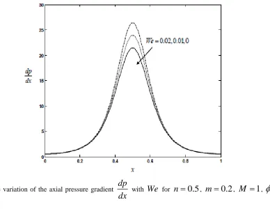
₀.

Fig. 2 illustrates the variation of the axial pressure gradient

dp

dx

with

We

for

n

=

0.5

,

m

=

0.2

,

M

=

1

,

0.5 φ

=

and

Q

= −

1

. It is observed that, the axial pressure gradient

dp

dx

increases with increasing Wiessenberg

number

We

.

The variation of the axial pressure gradient

dp

dx

with

n

for

We

=

0.01

,

m

=

0.2

,

M

=

1

,

φ

=

0.5

and

1 Q

= −

is depicted in Fig. 3. It is found that, the axial pressure gradient

dp

dx

decreases with an increase in power-law

index

n

.

Fig. 4 depicts the variation of the axial pressure gradient

dp

dx

with

m

for

n

=

0.5

,

We

=

0.01

,

M

=

1

,

0.5 φ

=

and

Q

= −

1

. It is noted that, the axial pressure gradient

dp

dx

decreases with increasing Hall parameter

m

.

The variation of the axial pressure gradient

dp

dx

with

M

for

n

=

0.5

,

m

=

0.2

,

We

=

0.01

,

φ

=

0.5

and

1 Q

= −

is shown in Fig. 5. It is observed that, on increasing Hartmann number

M

increases the axial pressure

gradient

dp

(7)

Fig. 6 shows the variation of the axial pressure gradient

dp

dx

with

φ

for

n

=

0.5

,

m

=

0.2

,

M

=

1

,

We

=

0.01

and Q= −1. It is found that, the axial pressure gradient dp

dx

increases with increasing amplitude ratio

φ

.

The variation of the pressure rise

∆

p

with

Q

for different values of

We

with

n

=

0.5

,

m

=

0.2

,

M

=

1

and

0.5 φ

=

is depicted in Fig. 7. It is noted that, the time-averaged volume flow rate Q increases with increasing Wiessenberg number

We

in pumping

(

∆ >

p

0 )

, free-pumping

(

∆ =

p

0 )

and co-pumping

(

∆ <

_p

₀

)

regions.

Fig. 8 illustrates the variation of the pressure rise

∆

p

with Q for different values of

n

with

We

=

0.01

,

m

=

0.2

,

M

=

1

and

φ

=

0.5

. It is found that, the time-averaged flow rate Q decreases with increasing

n

in both the pumping and free pumping regions, while it increases with increasing

n

in the co-pumping region.

∆

p

with

Q

m

with

n

=

0.5

,

We

=

0.01

,

M

=

1

and

0.5 φ

=

is illustrated in Fig. 9. It is observed that, the time-averaged flow rate

Q

decreases with increasing

m

in the pumping region, while it increases with increasing

m

in both the free pumping and co-pumping regions.

Fig. 10 depicts the variation of the pressure rise

∆

p

with

Q

M

with

n

=

0.5

,

m

=

0.2

,

0.01 We

=

and

φ

=

0.5

. It is noticed that, the time-averaged flow rate

Q

increases with increasing

M

in the pumping region, while it decreases with increasing

M

in both the free-pumping and co-pumping regions.

∆

p

with

Q

φ

with

n

=

0.5

,

m

=

0.2

,

M

=

1

and

0.01 We

=

is depicted in Fig. 11. It is observed that, the time-averaged flow rate

Q

φ

in both the pumping and free pumping regions, while it decreases with increasing

n

in the co-pumping region for chosen

( )

0 p

∆ <

.

Figs. 12-16 shows the variation of the friction force

F

with

Q

We

,

n

,

m

,

M

and

φ

. From these figures it is noted that there exists a critical value of

Q

below which F resists the flow and above which F

assist the flow.

Fig. 12 shows the variation of the friction force

F

with

Q

We

with

n

=

0.5

,

m

=

0.2

,

1 M

=

and

φ

=

0.5

. It is found that, the friction force

F

We

.

The variation of the friction force

F

with

Q

n

with

m

=

0.2

,

We

=

0.01

,

M

=

1

and

0.5 φ

=

is shown in Fig. 13. It is observed that below the critical value of

Q

, the friction force

F

n

, while above the critical value of

Q

it decreases with increasing

n

.

Fig. 14 depicts the variation of the friction force

F

with

Q

m

with

n

=

0.5

,

We

=

0.01

,

1 M

=

and

φ

=

0.5

. It is noted that below the critical value of

Q

F

m

, while above the critical value of

Q

it decreases with increasing

m

.

The variation of the friction force

F

with

Q

M

with

n

=

0.5

,

m

=

0.2

,

We

=

0.01

(8)

F

with

Q

φ

with

n

=

0.5

,

m

=

0.2

,

1 M

=

and

We

=

0.01

. It is found that below the critical value of

Q

F

decreases increasing

φ

,

while above the critical value of

Q

φ

.

5. CONCLUSIONS

In this paper, we investigated the effect of Hall on the peristaltic pumping of a hyperbolic tangent fluid in a planar channel under the assumption of long wavelength. The expressions for the velocity and axial pressure gradient are obtained by employing perturbation technique. It is found that, the axial pressure gradient and time-averaged flow rate in the pumping region increases with increasing the Weissenberg number

We

, the Hartmann number

M

and the amplitude ratio

φ

, while they decreases with increasing power-law index

n

and Hall parameter

m

. Also, it is found that below the critical value of

Q

the friction force

F

decreases with increasing

M

and

φ

while it increases with increasing

We n

,

and

m

; above the critical value of

Q

the friction force increases with increasing

We M

,

and

φ

while it decreases with increasing

n

and

m

. The results for Newtonian fluid can be obtained as the special cases of our analysis by choosing

M

=

0

,

n

=

0

and

We

=

0

.

Figure-2: The variation of the axial pressure gradient

dp

dx

with

We

for

n

=

0.5

,

m

=

0.2

,

M

=

1

,

φ

=

0.5

(9)

dp

dx

with

n

for

We

=

0.01

,

m

=

0.2

,

M

=

1

,

φ

=

0.5

and

Q

= −

1

.

dp

dx

with

m

for

n

=

0.5

,

We

=

0.01

,

M

=

1

,

φ

=

0.5

(10)

dp

dx

with

M

for

n

=

0.5

,

m

=

0.2

,

We

=

0.01

,

0.5 φ

=

and

Q

= −

1

.

dp

dx

with

φ

for

n

=

0.5

,

m

=

0.2

,

M

=

1

,

We

=

0.01

(11)

Figure-7: The variation of the pressure rise

∆

p

with

Q

We

with

n

=

0.5

,

m

=

0.2

,

1 M

=

and

φ

=

0.5

.

∆

p

with

Q

n

with

We

=

0.01

,

m

=

0.2

,

1

(12)

∆

p

with

Q

m

with

n

=

0.5

,

We

=

0.01

,

1 M

=

and

φ

=

0.5

.

∆

p

with

Q

M

with

n

=

0.5

,

m

=

0.2

,

0.01

(13)

∆

p

with

Q

φ

with

n

=

0.5

,

m

=

0.2

,

1 M

=

and

We

=

0.01

.

Figure-12: The variation of the friction force

F

with

Q

We

with

n

=

0.5

,

m

=

0.2

,

1

(14)

F

with

Q

n

with

m

=

0.2

,

We

=

0.01

,

1 M

=

and

φ

=

0.5

.

F

with

Q

m

with

n

=

0.5

,

We

=

0.01

,

1

(15)

F

with

Q

M

with

n

=

0.5

,

m

=

0.2

,

0.01 We

=

and

φ

=

0.5

.

F

with

Q

φ

with

n

=

0.5

,

m

=

0.2

,

1 M

=

and

We

=

0.01

.

REFERENCES

1. Ai, L. and Vafai, K. An investigation of Stokes’ second problem for non-Newtonian fluids, Numerical Heat Transfer, Part A, 47(2005), 955–980.

2. Akbar, N.S., Hayat, T., Nadeem, S. and Obaidat, S.

(16)

field, Math. Probl. Engng, 6 (2005), 663–677.

5. Gangavathi, P., Ramakrishna Prasad, A. and Subba Reddy, M. V. Effect of variable viscosity on the peristaltic flow of a Jeffrey fluid in a tube under the effect of a magnetic field: application to Adomian decomposition method, International Journal of Mathematical Archive, 3(6), 1-11.

6. Hayat, T and Ali, N. Peristaltically induced motion of a MHD third grade fluid in a deformable tube,

7. Hayat, T., Ali, N, and Asghar, S. Hall effects on peristaltic flow of a Maxwell fluid in a porous medium, Phys. Letters A, 363(2007), 397-403.

8. Jaffrin, M.Y. and Shapiro, A.H. Peristaltic Pumping, Ann. Rev. Fluid Mech., 3(1971), 13-36.

9. Li, A.A., Nesterov, N.I, Malikova, S.N. and Kilatkin, V.A. The use of an impulse magnetic field in the combined of patients with store fragments in the upper urinary tract. Vopr kurortol Fizide. Lech Fiz Kult, 3(1994), 22-24.

10. Nadeem, S. and Akbar, S. Numerical analysis of peristaltic transport of a Tangent hyperbolic fluid in an endoscope, Journal of Aerospace Engineering, 24(3) (2011), 309-317.

11. Nadeem, S. and Akram, S. Peristaltic transport of a hyperbolic tangent fluid model in an asymmetric channel, Z. Naturforsch., 64a (2009), 559 – 567.

12. Nadeem, S. and Akram, S. Magnetohydrodynamic peristaltic flow of a hyperbolic tangent fluid in a vertical asymmetric channel with heat transfer, Acta Mech. Sin., 27(2) (2011), 237–250.

13. Prasanth Reddy, D. and Subba Reddy, M.V. Peristaltic pumping of third grade fluid in an asymmetric channel under the effect of magnetic fluid, Advances in Applied Science Research, 3(6)(2012), 3868 – 3877.

14. Shapiro, A.H., Jaffrin, M.Y. and Weinberg, S.L. Peristaltic pumping with long wavelengths at low Reynolds number, J. Fluid Mech. 37(1969), 799-825.

Source of support: Nil, Conflict of interest: None Declared.