EVALUATION OF THE NON-ELEMENTARY INTEGRAL \(\int e^{\lambda x^\alpha}dx\), \(\alpha\ge 2\), AND OTHER RELATED INTEGRALS

EVALUATION OF THE NON-ELEMENTARY INTEGRAL

R

_e

dx

_,

α

_≥

_{2, AND OTHER RELATED INTEGRALS}

Victor Nijimbere

School of Mathematics and Statistics, Carleton University, Ottawa, Ontario, Canada

[email protected]

Abstract:A formula for the non-elementary integralReλxα

dxwhereαis real and greater or equal two, is obtained in terms of the confluent hypergeometric function1F1by expanding the integrand as a Taylor series. This result is verified by directly evaluating the area under the Gaussian Bell curve, corresponding toα= 2, using the asymptotic expression for the confluent hypergeometric function and the Fundamental Theorem of Calculus (FTC). Two different but equivalent expressions, one in terms of the confluent hypergeometric function1F1and another one in terms of the hypergeometric function1F2, are obtained for each of these integrals,

R

cosh(λxα

)dx, R

sinh(λxα

)dx,Rcos(λxα

)dxandRsin(λxα

)dx,λ∈C, α≥2. And the hypergeometric function1F2is expressed in terms of the confluent hypergeometric function1F1. Some of the applications of the non-elementary integral R

eλxα

dx, α≥2 such as the Gaussian distribution and the Maxwell-Bortsman distribution are given.

Key words:Non-elementary integral, Hypergeometric function, Confluent hypergeometric function, Asymp-totic evaluation, Fundamental theorem of calculus, Gaussian, Maxwell-Bortsman distribution.

1. Introduction

Definition 1. An elementary function is a function of one variable built up using that variable and constants, together with a finite number of repeated algebraic operations and the taking of exponentials and logarithms [6].

In 1835, Joseph Liouville established conditions in his theorem, known as Liouville 1835’s Theorem [4, 6], which can be used to determine whether an indefinite integral is elementary or non-elementary. Using Liouville 1835’s Theorem, one can show that the indefinite integral R

eλxαdx, α_≥2, is non-elementary [4], and to my knowledge, no one has evaluated this non-elementary integral before.

For instance, if α= 2, λ=₋β2 _{< 0, whereβ is a real constant, the area under the Gaussian}

Bell curve can be calculated using double integration and then polar coordinates to obtain

+∞

Z

−∞

e−β2x2dx=

√_π

β . (1.1)

Is that possible to evaluate (1.1) by directly using the Fundamental Theorem of Calculus (FTC) as in equation (1.2)?

+∞

Z

−∞

e−β2x2dx= lim

t→−∞

0 Z

t

e−β2x2dx+ lim

t→+∞

t

Z

0

The Central limit Theorem (CLT) in Probability theory [2] states that the probability that a random variablex does not exceed some observed value z is

P(X < z) = √1

2π

z

Z

−∞

e−x 2

2 dx. (1.3)

So if we know the antiderivative of the function g(x) = eλx2

, we may choose to use the FTC to calculate the cumulative probability P(X < z) in (1.3) when the value of z is given or is known, rather than using numerical integration.

The Maxwell-Boltsman distribution in gas dynamics,

F(v) =θ

v

Z

0

x2e−γx2dx, (1.4)

where θ and γ are some positive constants that depend on the properties of the gas and v is the gas speed, is another application.

There are many other examples where the antiderivative of g(x) = eλxα

, α_≥2 can be useful. For example, using the FTC, formulas for integrals such as

∞

Z

x

et2n+1dt, x <_∞;

∞

Z

x

e−t2n+1dt, x >_−∞;

∞

Z

x

t2ne−t2dt, x_{≤ ∞}, (1.5)

wherenis a positive integer, can be obtained if the antiderivative of g(x) =eλxα,α_≥2 is known. In this paper, the antiderivative of g(x) = eλxα, α _≥ 2, is expressed in terms of a special function, the confluent hypergeometric1F1 [1]. And the confluent hypergeometric 1F1 is an entire

function [3], and its properties are well known [1, 5]. The main goal here is to consider the most general case withλcomplex (λ_∈C_{), evaluate the non-elementary integral} R_eλxα_{,α≥2 and thus}

make possible the use of the FTC to compute the definite integral

B

Z

A

eλxαdx, (1.6)

for any A and B. And once (1.6) is evaluated, then integrals such as (1.1), (1.2), (1.3), (1.4) and (1.5) can also be evaluated using the FTC.

Using the hyperbolic and Euler identities,

cosh(λxα) = (eλxα +e−λxα)/2, sinh(λxα) = (eλxα ₋e−λxα)/2,

cos(λxα) = (eiλxα+e−iλxα)/2, sin(λxα) = (eiλxα ₋e−iλxα)/(2i),

the integrals

Z

cosh(λxα)dx, Z

sinh(λxα)dx, Z

cos(λxα)dx and

Z

sin(λxα)dx, α_≥2, (1.7)

are evaluated in terms of 1F1 for any constant λ. They are also expressed in terms of the

hyper-geometric1F2. And some expressions of the hypergeometric function 1F2 in terms of the confluent

hypergeometric function1F1 are therefore obtained.

For reference, we shall first define the confluent confluent hypergeometric function 1F1 and the hypergeometric function 1F2 before we proceed to the main aims of this paper (see sections 2

Definition 2. The confluent hypergeometric function, denoted as 1F1, is a special function given by the series [1, 5]

1F1(a;b;x) =

∞

X

n=0

(a)n

(b)n

xn

n!, (1.8)

where aand b are arbitrary constants, (ϑ)n= Γ(ϑ+n)/Γ(ϑ) (Pochhammer’s notation [1]) for any

complex ϑ, with (ϑ)0 = 1, and Γ is the standard gamma function [1].

Definition 3. The hypergeometric function1F2 is a special function given by the series [1, 5]

1F2(a;b, c;x) =

∞

X

n=0

(a)n

(b)n(c)n

xn

n!, (1.9)

where a, b and c are arbitrary constants, and (ϑ)n = Γ(ϑ+n)/Γ(ϑ) (Pochhammer’s notation [1])

as in Definition 2.

2. Evaluation of RB

A e λxα

dx

Proposition 1. The function G(x) = x 1F1 _α1;_α1 + 1;λxα, where 1F1 is a confluent hyper-geometric function [1], λis an arbitrarily constant and α_≥2, is the antiderivative of the function g(x) =eλxα. Thus,

Z

eλxαdx=x 1F1

1

α;

1

α + 1;λx

α

+C. (2.1)

P r o o f. We expand g(x) = eλxα

as a Taylor series and integrate the series term by term. We also use the Pochhammer’s notation [1] for the gamma function, Γ(a+n) = Γ(a)(a)n, where

(a)n =a(a+ 1)· · ·(a+n−1), and the property of the gamma function Γ(a+ 1) =aΓ(a) [1]. For

example, Γ(n+a+ 1) = (n+a)Γ(n+a). We then obtain

Z

g(x)dx=

Z

eλxαdx=

∞

X

n=0 λn

n!

Z

xαndx

=

∞

X

n=0 λn

n!

xαn+1

αn+ 1+C=

x α

∞

X

n=0

(λxα)n

n+_α1

n!+C

= x

α

∞

X

n=0

Γ n+_α1

Γ n+_α1 + 1

(λxα₎n

n! +C

=x

∞

X

n=0 1

α

n

1

α + 1

n

(λxα)n

n! +C

=x1F1

1

α;

1

α + 1;λx

α

+C=G(x) +C.

(2.2)

Example 1. We can now evaluateR

x2n_eλx2

dxin terms of the confluent hypergeometric function. Using integration by parts,

Z

x2neλx2dx= x

2n−1

2λ e

λx2

−2n₂−_λ1

Z

1. For instance, for n= 1,

Z

x2eλx2dx= x 2λe

λx2 −₂1_λ

Z

eλx2dx= x 2λe

λx2

−₂x_λ 1F1

1 2;

3 2;λx

2

+C. (2.4)

2. For n= 2,

Z

x4eλx2dx= x

3

2λe

λx2 − 3

2λ Z

x2eλx2dx= x

3

2λe

λx2 −3x

4λ2e

λx2

+3x 4λ2 1F1

1 2;

3 2;λx

2

+C. (2.5)

Example 2. Using the method of integrating factor, the first-order ordinary differential equation

y′+ 2xy = 1 (2.6)

has solution

y(x) =e−x2 Z

ex2dx+C

=xe−x2 1F1

1 2;

3 2;x

2

+Ce−x2. (2.7)

Assuming that the function G(x) (see Proposition 1) is unknown, in the following lemma, we use the properties of functiong(x) to establish the properties of G(x) such as the inflection points and the behavior as x_{→ ±∞}.

Lemma 1. Let the function G(x) be an antiderivative of g(x) =eλxα

, λ_∈C _withα≥2.

1. If the real part of λ is negative (< 0) and α is even, then the limits limx→−∞G(x) and

limx→+∞G(x) are finite (constants). And thus the Lebesgue integral

R∞

−∞|e

λxα

|dx <_∞.

2. If λ is real (λ _∈ R_{), then the point (0, G(0)) = (0,0) is an inflection point of the curve} Y =G(x), x_∈R_.

3. And if λ _∈R _{and λ < 0, and α is even, then the limits limx→−∞G(x) and limx→+∞G(x)}

are finite. And there exists real constant θ > 0 such that limits limx→−∞G(x) = −θ and

limx→+∞G(x) =θ.

P r o o f.

1. For complex λ = λr+iλi, where the subscript r and i stand for real and imaginary parts

respectively, the function g(x) = g(z) = ezα

where z = (λr +iλi)1/αx, α ≥ 2, is an entire

function on C_{. And if λr < 0 and α is even implies Re(z}α_{) is always negative regardless of}

the values of x. And so, if_|z_{| → ∞}(or x_{→ ±∞}), then g(z) = 0 (g(z) _→0) (or g(x) = 0 as

x _{→ ±∞}). Therefore by Liouville theorem, G(z) has to be constant as _|z_{| → ∞}, and so is

G(x) as x_{→ ±∞}. Hence, the Lebesgue integral

Z ∞

−∞|

eλxα_|dx=

Z ∞

−∞

eλrxα

|eλixα_|dx=

Z ∞

−∞

eλrxα

dx <_∞

sinceG(x) is constant as x_{→ ±∞}. For λr <0 andα odd, the limit limx→−∞eλrx

α

diverges and so does the integral R∞

−∞eλ

rxα_{dx. Therefore, the Lebesgue integral} R∞

−∞|eλx

α

|dx has to diverge too. On the other hand, for λr > 0, the limit limx→+∞eλrx

α

diverges, and so does the integral R∞

−∞eλ

rxα_{dxregardless of the value of α. Therefore, the Lebesgue integral}

R_∞

−∞|e

λxα

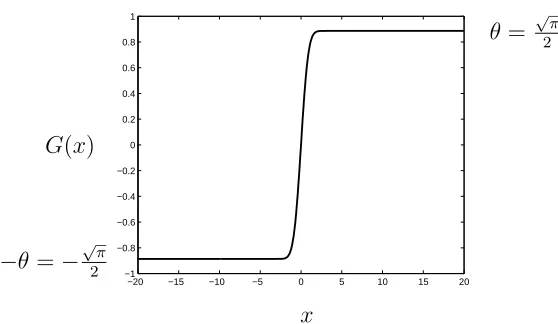
−20 −15 −10 −5 0 5 10 15 20 −1

−0.8 −0.6 −0.4 −0.2 0 0.2 0.4 0.6 0.8 1

G₍x₎

x

−θ ₌₋√π

2

θ₌ √π

2

Figure 1. G(x) is the antiderivative ofe−x2 _{given by (2.8).}

2. At x = 0, g(0) = 1. And so, around x = 0, the antiderivative G(x) _∼ x because G′_{(0) =}

g(0) = 1. And so (0, G(0)) = (0,0). Moreover, G′′_{(x) = g}′_{(x) = λαx}α−1_eλxα

, α _≥ 2, gives G′′_{(0) = 0. Hence, by the second derivative test, if λ is real (λ = λ}

r), the point

(0, G(0)) = (0,0) is an inflection point of the curve Y =G(x), x_∈R_.

3. For λ=λr (λ∈R), bothg(x) andG(x) are analytic onR. Using this fact and the fact that

for evenα andλr <0,

R_∞

−∞|e

λxα

|dx <_∞ implies that for evenαand λr <0,G(x) has to be

constant asx _{→ ±∞}. In addition, the fact that G′′_{(x)<0 if x <0 and G}′′_{(x) >0 ifx >0}

implies that, G(x) is concave upward on the interval (_∞,0) while is concave downward on the interval (0,+_∞). Moreover, the fact that g(x) = G′_{(x) is symmetric about the y-axis}

(even) implies thatG(x) has to be antisymmetric about they-axis (odd). Hence there exists a real positive constant θ >0 such that limits limx→−∞G(x)=−θand limx→+∞G(x)=θ.

Example 3. If λ=₋1 andα= 2, then

Z e−x2

dx=x 1F1

1 2;

3 2;−x

2

+C. (2.8)

According to (2.8), the antiderivative of g(x) =e−x2

is G(x) = x 1F1 1₂;3₂;−x2

. Its graph as a function ofx, sketched using MATLAB, is shown in Figure 1. It is in agreement with Lemma 1. It is actually seen in Figure 1 that (0,0) is an inflection point and thatG(x) reaches some constants asx_{→ ±∞}as predicted by Lemma 1.

In the following lemma, we obtain the values of G(x), the antiderivative of the function g(x) =

eλxα, as x_{→ ±∞}using the asymptotic expansion of the confluent hypergeometric function 1F1.

Lemma 2. Consider G(x) in Proposition 1.

1. Then for _|x_{| ≫}1,

G(x) =x1F1

1

α;

1

α + 1;λx

α

∼

   

  

Γ _α1 + 1ei

π α

λα1

x |x_|+

eλxα

αλxα−1,if α is even,

Γ _α1 + 1ei

π α

λα1

+ e

λxα

αλxα−1,if α is odd.

2. Let α_≥2 and be even, and let λ=₋β2, where β is a real number, preferably positive. Then

G(_−∞) = lim

x→−∞G(x) = limx→−∞x1F1

1

α;

1

α + 1;−β 2_xα

=₋ 1

βα2

Γ

1

α + 1

(2.10)

and

G(+_∞) = lim

x→+∞G(x) = limx→+∞x1F1

1

α;

1

α + 1;−β 2_xα

= 1

βα2

Γ

1

α + 1

. (2.11)

3. And by the FTC,

∞

Z

−∞

e−β2xαdx=G(+_∞)₋G(_−∞)

= 1

βα2

Γ

1

α + 1

− − 1 βα2

Γ

1

α + 1 !

= 2

βα2

Γ

1

α + 1

. (2.12)

P r o o f.

1. To prove (2.9), we use the asymptotic series for the confluent hypergeometric function that is valid for_|z_{| ≫}1 ([1], formula 13.5.1),

1F1(a;b;z)

Γ(b) =

e±iπa_z−a

Γ(b₋a)

(_R−1 X

n=0

(a)n(1 +a−b)n

n! (−z)

−n_+O(

|z_|−R)

)

+e

z_za−b

Γ(a)

(_S−1 X

n=0

(b₋a)n(1−a)n

n! (z)

−n_+O(

|z_|−S)

)

, (2.13)

where aand b are constants, and the upper sign being taken if ₋π/2<arg(z) <3π/2 and the lower sign if₋3π/2<arg(z)_{≤ −}π/2. We set z=λxα_{, a=} 1

α andb= α1 + 1, and obtain

1F1 _α1;_α1 + 1;λxα

Γ _α1 + 1 = eiπα

(λxα₎α1

(_R−1 X

n=0 1

α

n

n! (λx

α₎−n_+O{λxα₎−R

)

+e

λxα

(λxα)−1

Γ _α1

(_S−1 X

n=0

1₋ 1

α

n

(λxα)−n+O(λxα)−S

)

. (2.14)

Then, for_|x_{| ≫}1,

eiπα

(λxα₎1α

(_R−1 X

n=0 1

α

n

n! (λx

α₎−n_+O{λxα₎−R

)

∼

   

  

eiπα

λα1

1

|x_|,if α is even, eiπα

λα1

1

x,if α is odd,

(2.15)

while

eλxα(λxα)−1

Γ _α1

(_S−1 X

n=0

1₋ 1

α

n

(λxα)−n+O(λxα)−S

)

∼ e

λxα

Γ 1_α

And so, for_|x_{| ≫}1,

1F1 _α1;_α1 + 1;λxα

Γ _α1 + 1 ∼         

eiπα

λα1

1

|x_|+

eλxα

Γ _α1

λxα,if α is even,

eiπα

λα1

1

x +

eλxα

Γ _α1

λxα,if α is odd.

(2.17)

Hence,

G(x) =x1F1

1

α;

1

α + 1;λx

α ∼       

Γ _α1 + 1e

iπ α

λα1

x |x_|+

eλxα

αλxα−1,if α is even,

Γ _α1 + 1ei

π α

λα1

+ e

λxα

αλxα−1,if α is odd.

(2.18)

2. Setting λ=₋β2, whereβ is real and positive and using (2.9), then forα even,

G(x) =x1F1

1

α;

1

α + 1;−β 2_xα

∼ 1 βα2

Γ

1

α + 1

x |x_|−

e−β2_xα

αβ2_xα−1. (2.19)

Therefore,

G(_−∞) = lim

x→−∞G(x) = limx→−∞x1F1

1

α;

1

α + 1;−β 2_xα

=₋ 1

βα2

Γ

1

α + 1

(2.20)

and

G(+_∞) = lim

x→+∞G(x) = limx→+∞x1F1

1

α;

1

α + 1;−β 2_xα

= 1

βα2

Γ

1

α + 1

. (2.21)

3. By the Fundamental Theorem of Calculus, we have

+∞

Z

−∞

e−β2xαdx= lim

y→−∞

0 Z

y

e−β2xαdx+ lim

y→+∞

y

Z

0

e−β2xαdx

= lim

y→+∞y 1F1

1

α;

1

α + 1;−β 2_yα

− lim

y→−∞y 1F1

1

α;

1

α + 1;−β 2_yα

=G(+_∞)₋G(_−∞)

= 1

βα2

Γ

1

α + 1

− − 1 βα2

Γ

1

α + 1 !

= 2

βα2

Γ

1

α + 1

.

(2.22)

We now verify whether (2.22) is correct or not by double integration. We first observe that (2.22) is valid for all evenα_≥2. And so, if (2.22) is verified forα= 2, we are done since (2.22) is valid for all even α_≥2. Forα= 2, we have

+∞

Z

−∞

e−β2_x2

dx= lim

y→−∞

0 Z

y

e−β2_x2

dx+ lim

y→+∞

y

Z

0

e−β2_x2 dx

= lim

y→+∞y 1F1

1 2;

3 2;−β

2_y2

− lim

y→−∞y 1F1

1 2;

3 2;−β

2_y2

=G(+_∞)₋G(_−∞) = 2

On the other hand,





∞

Z

−∞

e−β2_x2 dx



 2

=





∞

Z

−∞

e−β2_x2 dx



 



∞

Z

−∞

e−β2_y2 dy



 (2.24)

=

∞

Z

−∞ ∞

Z

−∞

e−β2(x2+y2)dydx. (2.25)

In polar coordinate,

∞

Z

−∞ ∞

Z

−∞

e−β2(x2+y2)dydx=

2π

Z

0

∞

Z

0

e−β2r2rdrdθ = 1 2β2

2π

Z

0

dθ= π

β2. (2.26)

This gives

∞

Z

−∞

e−β2x2dx=

v u u u t

∞

Z

−∞ ∞

Z

−∞

e−(x2_+y2₎

dydx=

√ π

β (2.27)

as before.

Example 4. Setting λ=₋β2 =₋1,β= 1 and α= 2 in Lemma 2 gives

G(_−∞) = lim

x→−∞G(x) = limx→−∞x 1F1

1 2;

3 2;−x

2

=₋

√ π

2 (2.28)

and

G(+_∞) = lim

x→+∞G(x) = limx→+∞x 1F1

1 2;

3 2;−x

2

=

√ π

2 . (2.29) This impliesθ=√π/2 in Lemma 1. And this is exactly the value ofG(x) asx_{→ ∞} in Figure 1. We also have limx→−∞G(x) =−θ=−√π/2 as in Figure 1. Using the FTC, we readily obtain

0 Z

−∞

e−x2dx=G(0)₋G(_−∞) = 0₋

− √

π

2

=

√ π

2 , (2.30)

+∞

Z

0 e−x2

dx=G(+_∞)₋G(0) =

√ π

2 −0 =

√ π

2 (2.31)

and

+∞

Z

−∞

e−x2

dx=G(+_∞)₋G(_−∞) =

√_π

2 −

− √_π

2

=√π. (2.32)

Example 5. In this example, the integral

x

Z

−∞

wherenis a positive integer, is evaluated using Proposition 1 and the asymptotic expression (2.9). Settingλ= 1 and α= 2n+ 1 in Proposition 1 , and using (2.9) gives

x

Z

−∞

et2n+1dt= lim

y→−∞

x

Z

y

et2n+1dt

=x1F1

1 2n+ 1;

2n+ 2 2n+ 1;x

2n+1

− lim

y→−∞y 1F1

1 2n+ 1;

2n+ 2 2n+ 1;y

2n+1

=x1F1

1 2n+ 1;

2n+ 2 2n+ 1;x

2n+1

−Γ

2n+ 2 2n+ 1

, x <_∞.

(2.34)

One can also obtain

+∞

Z

x

e−t2n+1dt= lim

y→+∞

y

Z

x

e−t2n+1dt

= lim

y→−∞y 1F1

1 2n+ 1;

2n+ 2 2n+ 1;−y

2n+1

−x 1F1

1 2n+ 1;

2n+ 2 2n+ 1;−x

2n+1

= Γ

2n+ 2 2n+ 1

−x 1F1

1 2n+ 1;

2n+ 2 2n+ 1;−x

2n+1

, x >_−∞.

(2.35)

Theorem 1. For any A and B, the FTC gives

B

Z

A

eλxαdx=G(B)₋G(A), (2.36)

where G is the antiderivative of the function g(x) =eλxα

and is given in Proposition 1. And λ is any complex or real constant, and α_≥2.

P r o o f. G(x) = x 1F1 _α1;_α1 + 1;λxα, where λ is any constant, is the antiderivative of g(x) = eλxα, α _≥ 2 by Proposition 1, Lemma 1 and Lemma 2. And since the FTC works for

A=_−∞ and B = 0 in (2.30), A= 0 andB = +_∞ in (2.31) and A=_−∞ and B = +_∞ in (2.32) by Lemma 2 ifλ= 1 andα= 2, and for all λ <0 and all evenα _≥2, then it has to work for other values ofA, B _∈R_{and for any λ∈}C_{and α≥2. This completes the proof.}

Example 6. In this example, we apply Theorem 1 to the Central Limit Theorem in Probability theory [2]. The normal zero-one distribution of a random variable X is the measure µ(dx) =

gX(x)dx, where dx is the Lebesgue measure and the function gX(x) is the probability density

function (p.d.f) of the normal zero-one distribution [2], and is

gX(x) =

1

√

2πe

−x22,−∞< x <+∞. (2.37)

A comparison with the function g(x) in Proposition 1 and Lemma 1 gives λ = β2 = ₋1/2 and

P(X < z) =µ_{(_−∞, z)_}=

z

Z

−∞

gX(x)dx=

1

√

2π

z

Z

−∞

e−x22dx= 1

2 +

z √

2π 1F1

1 2;

3 2;−

z2

2

. (2.38)

For example, we can also use Theorem 1 to obtain P(₋2 < X < 2) = µ(₋2,2) = 0.4772 ₋ (₋0.4772) = 0.9544, P(₋1< X <2) =µ(₋1,2) = 0.4772₋(₋0.3413) = 0.8185 and so on.

Example 7. Using integration by parts and applying Theorem 1, the Maxwell-Bortsman distri-bution is written in terms of the confluent hypergeometric 1F1 as

F(v) =θ

v

Z

0

x2e−γx2dx=₋θv 2γe

−γv2

+ θv 2γ 1F1

1 2;

3 2;−γv

2

= θv 2γ

1F1

1 2;

3 2;−γv

2

−e−γv2

.

(2.39)

3. Other related non-elementary integrals

Proposition 2. The function G(x) = x 1F2

1

2α;12,21α + 1;λ

2_x2α

4

, where 1F2 is a hypergeo-metric function [1], λ is an arbitrarily constant and α _≥ 2, is the antiderivative of the function g(x) = cosh (λxα). Thus,

Z

cosh (λxα)dx=x 1F2

1 2α;

1 2,

1 2α + 1;

λ2_x2α

4

+C. (3.1)

P r o o f. We proceed as before. We expandg(x) = cosh (λxα_{) as a Taylor series and integrate}

the series term by term, use the Pochhammers notation [1] for the gamma function, Γ(a+n) = Γ(a)(a)n, where (a)n=a(a+ 1)· · ·(a+n−1), and the property of the gamma function Γ(a+ 1) =

aΓ(a) [1]. We also use the Gamma duplication formula [1]. We then obtain

Z

g(x)dx=

Z

cosh (λxα)dx=

∞

X

n=0 λ2n

(2n)!

Z

x2αndx

=

∞

X

n=0 λ2n

(2n)!

x2αn+1

2αn+ 1 +C

= x 2α

∞

X

n=0

(λ2x2α)n

(2n)! n+₂1_α +C

= x 2α

∞

X

n=0

Γ n+ ₂1_α

Γ(2n+ 1)Γ n+₂1_α + 1(λ

2_x2α₎n_+C

=x

∞

X

n=0

1 2α

n

1 2

n

1 2α+ 1

n

(λ2_x2α₎n

n! +C

=x 1F2

1 2α;

1 2,

1 2α + 1;

λ2x2α

4

+C=G(x) +C.

(3.2)

Proposition 3. The function

G(x) = λx

α+1 α+ 1 1F2

1 2α +

1 2;

3 2,

1 2α +

3 2;

λ2_x2α

4

where1F2 is a hypergeometric function[1], λis an arbitrarily constant andα_≥2, is the antideriva-tive of the function g(x) = sinh (λxα). Thus,

Z

sinh (λxα)dx= λx

α+1 α+ 1 1F2

1 2α +

1 2;

3 2,

1 2α +

3 2;

λ2_x2α

4

+C. (3.3)

P r o o f. As above, we expand g(x) = sinh (λxα_{) as a Taylor series and integrate the series}

term by term, use the Pochhammers notation [1] for the gamma function, Γ(a+n) = Γ(a)(a)n,

where (a)n = a(a+ 1)· · ·(a+n−1), and the property of the gamma function Γ(a+ 1) =aΓ(a)

[1]. We also use the Gamma duplication formula [1]. We then obtain

Z

g(x)dx=

Z

sinh (λxα)dx=

∞

X

n=0

λ2n+1

(2n+ 1)!

Z

x2αn+αdx

=

∞

X

n=0

λ2n+1

(2n+ 1)!

x2αn+α+1

2αn+α+ 1+C

= λx α+1 2α ∞ X n=0

(λ2x2α)n

(2n+ 1)! n+ ₂1_α +1₂ +C

= λx α+1 2α ∞ X n=0

Γ n+₂1_α +1₂

Γ(2n+ 2)Γ n+₂1_α+ 3₂(λ

2_x2α₎n_+Cr

= λx

α+1 α+ 1

∞

X

n=0 1 2α +12

n 3 2 n 1 2α +32

n

(λ2_x2α₎n

n! +C

= λx

α+1 α+ 1 1F2

1 2α +

1 2;

3 2,

1 2α +

3 2;

λ2x2α

4

+C=G(x) +C.

(3.4)

We also can show as above that

Z

cos (λxα)dx=x 1F2

1 2α;

1 2,

1

2α + 1;− λ2x2α

4

+C (3.5)

and

Z

sin (λxα)dx= λx

α+1 α+ 1 1F2

1 2α +

1 2;

3 2,

1 2α +

3 2;−

λ2_x2α

4

+C. (3.6)

Theorem 2. For any constants α and λ,

1F2

1 2α;

1 2,

1 2α + 1;

λ2x2α

4

= 1 2

1F1

1

α;

1

α + 1;λx

α

+ 1F1

1

α;

1

α + 1;−λx

α

(3.7)

and

1F2

1 2α;

1 2,

1

2α + 1;− λ2_x2α

4

= 1 2

1F1

1

α;

1

α + 1;iλx

α

+ 1F1

1

α;

1

α + 1;−iλx

α

. (3.8)

P r o o f. Using Proposition 1, we obtain

Z

cosh (λxα)dx=

Z

eλxα+e−λxα

2 dx = x 2 1F1 1 α; 1

α + 1;λx

α + 1F1 1 α; 1

α + 1;−λx

α

Hence, comparing (3.1) with (3.9) gives (3.7). Using Proposition 1, on the other hand, we obtain

Z

cos (λxα)dx=

Z

eiλxα+e−iλxα

2 dx

= x 2

1F1

1

α;

1

α + 1;iλx

α

+ 1F1

1

α;

1

α + 1;−iλx

α

+C. (3.10)

Hence, comparing (3.5) with (3.10) gives (3.8).

Theorem 3. For any constants α and λ,

λxα α+ 1 1F2

1 2α +

1 2;

3 2,

1 2α +

3 2;−

λ2x2α

4

= 1 2

1F1

1

α;

1

α + 1;λx

α

− 1F1

1

α;

1

α + 1;−λx

α

(3.11)

and

λxα α+ 1 1F2

1 2α +

1 2;

3 2,

1 2α +

3 2;−

λ2x2α

4

= 1 2i

1F1

1

α;

1

α + 1;iλx

α

− 1F1

1

α;

1

α + 1;−iλx

α

. (3.12)

P r o o f. Using Proposition 1, we obtain

Z

sinh (λxα)dx=

Z

eλxα+e−λxα

2 dx

= x 2

1F1

1

α;

1

α+ 1;λx

α

− 1F1

1

α;

1

α + 1;−λx

α

+C. (3.13)

Hence, comparing (3.3) with (3.13) gives (3.11). Using Proposition 1, on the other hand, we obtain

Z

sin (λxα)dx=

Z

eiλxα +e−iλxα

2i dx

= x 2i

1F1

1

α;

1

α + 1;iλx

α

− 1F1

1

α;

1

α + 1;−iλx

α

+C. (3.14)

Hence, comparing (3.6) with (3.14) gives (3.12).

4. Conclusion

The non-elementary integral R

eλxαdx, where λ is an arbitrary constant and α _≥ 2, was ex-pressed in term of the confluent hypergeometric function 1F1. And using the properties of the

than using double integration and then polar coordinates. One can also choose to use Theorem 1 to compute the cumulative probability for the normal distribution or that for the Maxwell-Bortsman distribution as shown in examples 6 and 7.

On one hand, the integrals R

cosh(λxα)dx, R

sinh(λxα)dx, R

cos(λxα)dx and R

sin(λxα)dx, α_≥2, were evaluated in terms of the confluent hypergeometric function 1F1, while on another

hand, they were expressed in terms of the hypergeometric1F2. This allowed to express the

hyper-geometric function1F2 in terms of the confluent hypergeometric function 1F1 (Theorems 2 and 3).

REFERENCES

1. Abramowitz M., Stegun I.A.Handbook of mathematical functions with formulas, graphs and math-ematical tables. National Bureau of Standards, 1964. 1046 p.

2. Billingsley P. Probability and measure. Wiley series in Probability and Mathematical Statistics, 3rd Edition, 1995. 608 p.

3. Krantz S.G.Handbook of complex variables. Boston: MA Birkh¨auser, 1999. 290 p. DOI: 10.1007/978-1-4612-1588-2

4. Marchisotto E.A., Zakeri G.-A. An invitation to integration in finite terms // College Math. J., 1994. Vol. 25, no. 4. P. 295–308. DOI: 10.2307/2687614

5. NIST Digital Library of Mathematical Functions.http://dlmf.nist.gov/