Vol 8, No 11 (2017)

Available online throug

ISSN 2229 – 5046

International Journal of Mathematical Archive- 8(11), Nov. – 2017 155

EOQ INVENTORY MODEL FOR TIME DEPENDENT DETERIORATING ITEMS

WITH QUADRATIC TIME VARYING DEMAND, TWO PARAMETER WEIBULL

DETERIORATION AND PARTIAL BACKLOGGING

R. KAVITHA PRIYA*

_{, Dr. K. SENBAGAM}

1

_{Department of Mathematics,}

CSI College of Engineering, Ketti, The Nilgiris, Tamil Nadu, India.

2

_{Department of Mathematics,}

PSG College of Arts and Science, Coimbatore, Tamil Nadu, India.

(Received On: 30-10-17; Revised & Accepted On: 16-11-17)

ABSTRACT

P

considered an inventory model with random lifetime that is, the deterioration rate follows a two parameter Weibull distribution. The demand rate is assumed to be a quadratic function of time. The shortages are allowed. All demands are satisfied immediately by partial backlogging.The proposed model is approved with a numerical example. The sensitivity analysis is provided to examine the impact of changes with the variation in the parameters each at a time on the optimal solution.

Keywords: Deteriorating items, Weibull distribution, quadratic demand, shortages, partial backlogging.

1. INTRODUCTION

One of the assumptions of conventional inventory models was that the items preserve their unique characteristics throughout when they are kept in the inventory. This assumption is true for most of the items, but not for all. Most of the physical merchandise like vegetables, fruits, food grains, medicine, fashion goods, chemicals, etc. deteriorate over time. They either get rotted, damaged, vaporized or influenced by some factors and do not remain in an ideal condition to satisfy the demand. In general, most physical goods will deteriorate during storage and customers are less likely to buy deteriorated goods .The value of goods will decline or even be lost. Vendors therefore have to reduce the price of deteriorated goods in order to sell them. The economic loss necessitates the more detailed consideration of deterioration.

Many researchers like Aggarwal [1], Panda et al. [12], Venkateswarlu & Mohan [28] have studied the constant rate of deterioration in their models. Berrotoni [4] was the first to discuss the difficulties of fitting experimental data to mathematical distribution since the rate of deterioration increases with age. For items such as steel, equipment, crystal and toys, the rate of deterioration is very less, which requires very little consideration of deterioration. But some items such as fruits, vegetables and medicine have remarkable deterioration overtime. It has been noticed that the deterioration of many such items can be well expressed by Weibull distribution. This prompted Covert & Philip [8] to build an inventory model for deteriorating items following two parameter Weibull distribution. Later Philip [21] extended this model by considering Weibull distribution with three parameters. Mishra [26] developed an EOQ model for deteriorating item with two parameter Weibull distribution where the allowed shortages are partially backlogged. Begum et al. [2] have considered the two parameter Weibull distribution with the production rate and demand rate being inversely proportional to each other.

Corresponding Author: R. Kavitha Priya*

_,

Demand is the major factor in the inventory management. Hence, problems in inventory should be handled by considering both present and future demands. Demand may be constant or varying with time, stock, price, etc. The constant demand is possible only when the life cycle of the product is completed with limited time periods. Bakker et al. [18], in their article, divided the demand into, deterministic and stochastic demand. Before ordering of inventory, the deterministic demand is known while the stochastic demand is not known. Most of the authors considered constant demand or stock dependent demand. Dave & Patel [9] put forward an inventory model for disintegrating items with time related demand, instantaneous replenishment of stock, not allowing shortages. While analysing the time variant demand pattern, the researcher normally considers an exponential demand rate. Hariga & Benkherouf [13] developed the stock model with exponential demand which is time variant. The exponential declining demand was studied by authors like Ouang & Cheng [19], Sarala & Garima [23] and Bhanupriya et al. [5]. An exponential rate of change in demand was observed to be exceptionally high and the demand variation of any material in the genuine market cannot be so high. Jalan & Chaudhuri [15] developed an inventory model for deteriorating items with exponential degradation, immediate replenishment and time dependent linear demand rate. Chung & Ting [7] have also considered the linear demand pattern in their model. The primary impediment in linear time-varying demand rate is that it implies a steady change in the demand rate per unit time. This rarely happens in the case of any commodity in the market. Tripathi & Pandey [25] presented a model based on a Weibull time dependent demand rate for non-deteriorating items when the supplier provides trade credits. Gino et al. [11], Karmakar & Choudhury [5] and Kun Shan Wu [17] have presented an inventory model for items with Weibull distribution deterioration, ramp type demand rate and partial backlogging.

presented that a practical approach to the quickened increase or decrease in the demand rate can be well represented by a quadratic function of time. Ghosh & Chaudhuri [10] have studied the quadratic demand with two parameter Weibull distributed deterioration. Vandana & Sharma [27] have proposed a stock model for deteriorating items which do not deteriorate instantly, with quadratic demand rate under trade credit policy. Rangarajan & Karthikeyan [22] have developed and analysed the inventory model for deteriorating item with time dependent holding cost and different demand rates such as constant, linear and quadratic demand rates without allowing shortages. They have concluded that if the demand rate is taken as constant then the total cost is very low and cycle period is long. If the demand rate is taken as linear or quadratic then the total cost is high but cycle period is short. We realize that the shortages in stock framework are either completely backlogged or totally lost. It is more sensible to portray that when the waiting time for the next replenishment is extended, the backlogging rate would become lesser, for commodities with increase in sales. Thus, the rate of backlogging is dependent on the duration of the waiting time for the next renewal. Park [20] has displayed a stock model in which, during the out of stock period, the demand is partly backordered and the remaining is lost. Begum et al. [3], Sarkar et al. [24] and Jagadeeswari & Chenniappan [14] have established an order level inventory model for deteriorating items with quadratic demand and partial backlogging.

In the present article we have discussed the inventory model for deteriorating items having Weibull distribution deterioration and the demand following the quadratic pattern. The shortages are permitted and are partially backlogged.

2. ASSUMPTIONS

• Lead time is zero. • Time horizon is infinite.

• 𝐷(𝑡) =𝑎+𝑏𝑡+𝑐𝑡2_{,𝑎 ≥0,𝑏 ≠0,𝑐 ≠0 : Demand rate is time dependent, where a is the initial rate of}

demand, b is the rate with which the demand rate increases. The rate of change in the demand rate itself increases at a rate c.

• _{𝜃(𝑡) =𝛼𝛽𝑡}𝛽−1_{: Deterioration rate which follows a two parameter Weibull distribution, where 0≤ 𝛼< 1 is}

the scale parameter, 𝛽> 0 is the shape parameter and 0≤ 𝜃(𝑡) < 1. If 0 <𝛽< 1 then θ(t) decreases with time, if 𝛽= 1, then θ(t) is constant and if 𝛽> 1 then θ(t)increases with time.

• Shortages are allowed.

• Unsatisfied demand is backlogged, and the fraction of shortages backordered is 1

1+𝛿(𝑇−𝑡)where T is the waiting time for the next replenishment and 𝛿 is a positive constant. Therefore, if customers do not need to wait, then no sales are lost, and all sales are lost if customers are faced with an infinite wait.

3 . NOTATIONS

• 𝐶1 : Holding cost per unit per unit time.

• _𝐶2 : Cost of the inventory per unit. • _𝐶3 : Ordering cost of inventory per order. • _𝐶4 : Shortage cost per unit per unit time. • _𝐶5 : Opportunity cost due to lost sales per unit.

© 2017, IJMA. All Rights Reserved 157

• _𝑇 : Length of each ordering cycle.

• _𝑊 : The maximum inventory level for each ordering cycle.

• _𝑆 : The maximum amount of demand backlogged for each ordering cycle. • _𝑄 : The order quantity for each ordering cycle.

• 𝐼(𝑡) : The inventory level at time 𝑡 , 0≤ 𝑡 ≤ 𝑇. • _𝛼 : Scale parameter.

• _𝛽 : Shape parameter.

• _𝑡1∗ _{: The optimal solution of 𝑡} 1.

• _𝑇∗ _{: The optimal solution of𝑇.}

• _𝑇𝐶∗ _{: The average total cost per unit time.}

4. MATHEMATICAL FORMULATION

This paper is developed to determine the total cost (TC) for items having time dependent quadratic demand and deterioration following Weibull distribution allowing shortages which are backlogged.

As the inventory level reduces due to deterioration and demand rate during the interval [𝑡1,𝑇] the governing differential equation of the inventory level at time 𝑡 isas follows:

𝑑𝐼(𝑡)

𝑑𝑡 +𝛼𝛽𝑡𝛽−1𝐼(𝑡) =−(𝑎+𝑏𝑡+𝑐𝑡2), 0≤ 𝑡 ≤ 𝑡1. (1)

The solution of equation (1) with boundary condition 𝐼(𝑡) = 0, is

𝐼(𝑡)𝑒∫ 𝛼𝛽𝑡𝛽−1_{=� −(𝑎+𝑏𝑡+𝑐𝑡}2_)𝑒∫ 𝛼𝛽𝑡𝛽−1_𝑑𝑡

𝐼(𝑡) 𝑒𝛼𝑡𝛽

= − �∫(𝑎+𝑏𝑡+𝑐𝑡2)�1 +𝛼𝑡𝛽

1!� 𝑑𝑡 �

=− ��𝑎+𝑎𝛼𝑡𝛽_{+𝑏𝑡+𝑏𝛼𝑡}𝛽+1_+𝑐𝑡2_{+𝑐𝛼𝑡}𝛽+2_{� 𝑑𝑡}

=− �𝑎(𝑡 − 𝑡1) +𝑎 �𝛼𝑡_{𝛽+ 1}𝛽+1−𝛼𝑡_𝛽1_{+ 1}𝛽+1�+𝑏 �𝑡₂2−𝑡₂12�+𝑏 �𝛼𝑡_{𝛽+ 2}𝛽+2−𝛼𝑡_𝛽1_{+ 2}𝛽+2�+𝑐 �𝑡₃3−𝑡1₃3�

+𝑐 �𝛼𝑡_{𝛽+ 3}𝛽+3−𝛼𝑡_𝛽1_{+ 3}𝛽+3��

=�𝑎 �𝑡1+𝛼𝑡1 𝛽+1

𝛽+ 1�+𝑏 �

𝑡12 2 +

𝛼𝑡1𝛽+2

𝛽+ 2�+𝑐 �

𝑡13 3 +

𝛼𝑡1𝛽+3

𝛽+ 3��

− �𝑎 �𝑡+𝛼𝑡_{𝛽+ 1}𝛽+1�+𝑏 �𝑡_{2 +}2 𝛼𝑡_{𝛽+ 2}𝛽+2�+𝑐 �𝑡_{3 +}3 𝛼𝑡_{𝛽+ 3}𝛽+3��

𝐼(𝑡) =�𝑎 �𝑡1+𝛼𝑡1 𝛽+1

𝛽+ 1�+𝑏 �

𝑡12 2 +

𝛼𝑡1𝛽+2

𝛽+ 2�+𝑐 �

𝑡13 3 +

𝛼𝑡1𝛽+3

𝛽+ 3�� 𝑒−𝛼𝑡

𝛽

− �𝑎 �𝑡+𝛼𝑡𝛽+1

𝛽+1�+ 𝑏 � 𝑡2

2 + 𝛼𝑡𝛽+2

𝛽+2 �+𝑐 � 𝑡3

3 + 𝛼𝑡𝛽+3

𝛽+3 �� 𝑒−𝛼𝑡

𝛽

, 0≤ 𝑡 ≤ 𝑡₁ (2)

Maximum inventory level for each cycle is obtained by putting the boundary condition 𝐼(0) =𝑊 in equation (2). Therefore,

𝐼(0) =𝑊=�𝑎 �𝑡1+𝛼𝑡1

𝛽+1

𝛽+1 �+𝑏 � 𝑡12

2 + 𝛼𝑡1𝛽+2

𝛽+2 �+𝑐 � 𝑡13

3 + 𝛼𝑡1𝛽+3

𝛽+3 �� (3)

During the shortage interval (𝑡1,𝑇) the demand at time 𝑡 is partially backlogged at the fraction 1

1+𝛿(𝑇−𝑡) .

Therefore, the differential equation governing the amount of demand backlogged is

𝑑𝐼(𝑡)

𝑑𝑡 =− 𝐷0

1+𝛿(𝑇−𝑡),𝑡1≤ 𝑡 ≤ 𝑇 (4) With the boundary condition 𝐼(𝑡1) = 0.

The solution of equation (4) is 𝐼(𝑡) =𝐷0

𝛿 𝑙𝑛(1 +𝛿(𝑇 − 𝑡))− 𝐷0

𝛿 𝑙𝑛(1 +𝛿(𝑇 − 𝑡1)), 𝑡1≤ 𝑡 ≤ 𝑇 (5)

Maximum amount of demand backlogged per cycle is obtained by putting 𝑡=𝑇 in equation (5). Therefore, 𝑆=−𝐼(𝑡) =𝐷0

Hence, the economic order quantity per cycle is 𝑄=𝑊+𝑆=�𝑎 �𝑡1+𝛼𝑡1

𝛽+1

𝛽+1 �+𝑏 � 𝑡12

2 + 𝛼𝑡1𝛽+2

𝛽+2 �+𝑐 � 𝑡13

3 + 𝛼𝑡1𝛽+3

𝛽+3 ��+ 𝐷0

𝛿 𝑙𝑛(1 +𝛿(𝑇 − 𝑡1)) (7)

The inventory holding cost per cycle is

𝐻𝐶=𝐶1� 𝐼(𝑡)𝑑𝑡 𝑡1

0

=𝐶1� �𝑎 �𝑡1+𝛼𝑡1 𝛽+1

𝛽+ 1�+𝑏 �

𝑡12 2 +

𝛼𝑡1𝛽+2

𝛽+ 2�+𝑐 �

𝑡13 3 +

𝛼𝑡1𝛽+3

𝛽+ 3�� 𝑡1

0

𝑒−𝛼𝑡𝛽

𝑑𝑡

− 𝐶1� �𝑎 �𝑡+𝛼𝑡 𝛽+1

𝛽+ 1�+𝑏 �

𝑡2 2 +

𝛼𝑡𝛽+2

𝛽+ 2�+𝑐 �

𝑡3 3 +

𝛼𝑡𝛽+3

𝛽+ 3�� 𝑡1

0

𝑒−𝛼𝑡𝛽

𝑑𝑡

=𝐶1� �𝑎𝑡1− 𝑎𝑡+𝑏𝑡1 2 2 − 𝑏

𝑡2 2 +𝑐

𝑡13 3 − 𝑐

𝑡3 3 +𝑎

𝛼𝑡1𝛽+1

𝛽+ 1 − 𝑎

𝛼𝑡𝛽+1

𝛽+ 1 +𝑏

𝛼𝑡1𝛽+2

𝛽+ 2 − 𝑏

𝛼𝑡𝛽+2

𝛽+ 2 +𝑐

𝛼𝑡1𝛽+3

𝛽+ 3 𝑡1

0

− 𝑐𝛼𝑡_{𝛽+ 3}𝛽+3� �1− 𝛼𝑡𝛽_�𝑑𝑡

=𝐶1� �𝑎𝑡1− 𝑎𝑡+𝑏𝑡1 2 2 − 𝑏

𝑡2 2 +𝑐

𝑡13 3 − 𝑐

𝑡3 3 +𝑎

𝛼𝑡1𝛽+1

𝛽+ 1 − 𝑎

𝛼𝑡𝛽+1

𝛽+ 1 +𝑏

𝛼𝑡1𝛽+2

𝛽+ 2 − 𝑏

𝛼𝑡𝛽+2

𝛽+ 2 +𝑐

𝛼𝑡1𝛽+3

𝛽+ 3 𝑡1

0

− 𝑐𝛼𝑡_{𝛽+ 3}𝛽+3− 𝑎𝑡1𝛼𝑡𝛽+𝑎𝛼𝑡𝛽+1− 𝑏𝑡1 2_𝛼𝑡𝛽

2 +𝑏

𝛼𝑡𝛽+2

2 − 𝑐

𝑡13𝛼𝑡𝛽

3 +𝑐

𝛼𝑡𝛽+3

3 − 𝑎

𝛼2_𝑡 1𝛽+1𝑡𝛽

𝛽+ 1 +𝑎𝛼_𝛽2𝑡_{+ 1}2𝛽+1− 𝑏𝛼2_𝛽𝑡1_{+ 2 +}𝛽+2𝑡𝛽 𝑏𝛼_𝛽2𝑡_{+ 2}2𝛽+2− 𝑐𝛼2_𝛽𝑡1_{+ 3 +}𝛽+3𝑡𝛽 𝑐𝛼_𝛽2𝑡_{+ 3}2𝛽+3� 𝑑𝑡

=𝐶1�𝑎𝑡1 2 2 +

𝑏𝑡13 3 +

𝑐𝑡14 4 +

𝑎𝛼𝛽

(𝛽+ 1)(𝛽+ 2)𝑡1𝛽+2+

𝑏𝛼𝛽

(𝛽+ 1)(𝛽+ 3)𝑡1𝛽+3+

𝑐𝛼𝛽

(𝛽+ 1)(𝛽+ 4)𝑡1𝛽+4

−_{(𝛽+ 1)(2}𝑎𝛼2_{𝛽+ 2)}𝑡12𝛽+2− 𝑏𝛼 2

(𝛽+ 1)(2𝛽+ 3)𝑡12𝛽+3−

𝑐𝛼2

(𝛽+ 1)(2𝛽+ 4)𝑡12𝛽+4� (8)

The deterioration cost per cycle is

𝐷𝐶 =𝐶2�𝑊 − � 𝐷(𝑡)𝑑𝑡 𝑡1

0

�

=𝐶2�𝑊 − �(𝑎+𝑏𝑡+𝑐𝑡2)𝑑𝑡 𝑡1

0

�

=𝐶2�𝑎 �𝑡1+𝛼𝑡1 𝛽+1

𝛽+ 1�+𝑏 �

𝑡12 2 +

𝛼𝑡1𝛽+2

𝛽+ 2�+𝑐 �

𝑡13 3 +

𝛼𝑡1𝛽+3

𝛽+ 3� − 𝑎𝑡1−

𝑏𝑡12

2 −

𝑐𝑡13 3 � =𝛼𝐶2�𝑎𝑡1

𝛽+1

𝛽+1 + 𝑏𝑡1𝛽+2

𝛽+2 + 𝑐𝑡1𝛽+3

𝛽+3 � (9)

The shortage cost per cycle is

𝑆𝐶=𝐶4�� 𝐼(𝑡)𝑑𝑡 𝑇

𝑡1

�

=𝐶4_{𝛿 ��}𝐷0 ln�1 +𝛿(𝑇 − 𝑡)� −ln (1 +𝛿(𝑇 − 𝑡1))�𝑑𝑡

𝑇

𝑡1

=𝐶4𝐷0�𝑇−𝑡_𝛿1−_𝛿12ln�1 +𝛿(𝑇 − 𝑡1)�� (10)

The opportunity cost due to lost sales per cycle is

𝑂𝐶=𝐶5� 𝐷0�1−_{1 +𝛿(}1_{𝑇 − 𝑡)}� 𝑑𝑡 𝑇

𝑡1

© 2017, IJMA. All Rights Reserved 159

Therefore, the average total cost per unit time per cycle = (holding cost + deterioration cost + ordering cost + shortage cost + opportunity cost due to lost sales) / length of the ordering cycle, i.e,

𝑇𝐶=1_𝑇�𝐶1�𝑎𝑡1 2 2 +

𝑏𝑡13 3 +

𝑐𝑡14 4 +

𝑎𝛼𝛽

(𝛽+ 1)(𝛽+ 2)𝑡1𝛽+2+_{(𝛽+ 1)(}𝑏𝛼𝛽_{𝛽+ 3)}𝑡1𝛽+3+_{(𝛽+ 1)(}𝑐𝛼𝛽_{𝛽+ 4)}𝑡1𝛽+4

−_{(𝛽+ 1)(2}𝑎𝛼2_{𝛽+ 2)}𝑡12𝛽+2− 𝑏𝛼 2

(𝛽+ 1)(2𝛽+ 3)𝑡12𝛽+3− 𝑐𝛼 2

(𝛽+ 1)(2𝛽+ 4)𝑡12𝛽+4� +𝛼𝐶2�𝑎𝑡1

𝛽+1

𝛽+ 1 +

𝑏𝑡1𝛽+2

𝛽+ 2 +

𝑐𝑡1𝛽+3

𝛽+ 3�+𝐶3+𝐶4𝐷0�

𝑇 − 𝑡1

𝛿 −

1

𝛿2ln�1 +𝛿(𝑇 − 𝑡1)��

+𝐶5𝐷0�𝑇 − 𝑡1−1_{𝛿 𝑙𝑛�}1 +𝛿(𝑇 − 𝑡1)���

=_𝑇1

⎣ ⎢ ⎢ ⎢ ⎢ ⎡

𝐶1�

𝑎 �𝑡12

2 + 𝛼𝛽

(𝛽+1)(𝛽+2)𝑡1𝛽+2−

𝛼2

(𝛽+1)(2𝛽+2)𝑡12𝛽+2�+𝑏 �

𝑡13

3 + 𝛼𝛽

(𝛽+1)(𝛽+3)𝑡1𝛽+3−

𝛼2

(𝛽+1)(2𝛽+3)𝑡12𝛽+3�

+𝑐 �𝑡14

4 + 𝛼𝛽

(𝛽+1)(𝛽+4)𝑡1𝛽+4−

𝛼2

(𝛽+1)(2𝛽+4)𝑡12𝛽+4�

�

+𝛼𝐶2�𝑎𝑡1

𝛽+1

𝛽+1 + 𝑏𝑡1𝛽+2

𝛽+2 + 𝑐𝑡1𝛽+3

𝛽+3 �+𝐶3+

𝐷0(𝐶4+𝛿𝐶5)

𝛿 (𝑇 − 𝑡1)−

𝐷0(𝐶4+𝛿𝐶5)

𝛿2 ln�1 +𝛿(𝑇 − 𝑡1)� _⎦⎥

⎥ ⎥ ⎥ ⎤ (12) Now, 𝜕𝑇𝐶 𝜕𝑡1 =

𝐶1 𝑇 ⎣ ⎢ ⎢ ⎢

⎡𝑎 �𝑡1+_(𝛽𝛼𝛽_{+ 1)}𝑡1𝛽+1− 𝛼 2

(𝛽+ 1)𝑡12𝛽+1�+𝑏 �𝑡12+

𝛼𝛽

(𝛽+ 1)𝑡1𝛽+2−

𝛼2

(𝛽+ 1)𝑡12𝛽+2�

+𝑐 �𝑡14+_(𝛽𝛼𝛽_{+ 1)}𝑡1𝛽+3− 𝛼 2

(𝛽+ 1)𝑡12𝛽+3� _⎦⎥

⎥ ⎥ ⎤

+1_𝑇�𝛼𝐶2�𝑎𝑡1𝛽+𝑏𝑡1𝛽+1+𝑏𝑡1𝛽+1��+_𝛿𝑇𝐷0(−𝐶4− 𝛿𝐶5) +_𝛿𝐷20_𝑇(𝐶4+𝛿𝐶5)

𝛿

�1+𝛿(𝑇−𝑡1)� (13)

The optimum values of 𝑡₁ and 𝑇 in order to minimize the average total cost are the solutions of the equations

𝜕𝑇𝐶

𝜕𝑡1 = 0 and

𝜕𝑇𝐶

𝜕𝑇 = 0 (14)

Provided that they satisfy the sufficient conditions

𝜕2_(𝑇𝐶)

𝜕𝑡12 > 0,

𝜕2_(𝑇𝐶)

𝜕𝑇2 > 0 and�

𝜕2_(𝑇𝐶)

𝜕𝑡12 �.�

𝜕2_(𝑇𝐶)

𝜕𝑇2 � − �

𝜕2_(𝑇𝐶)

𝜕𝑡1𝜕𝑇�

2 > 0.

Equation (13) can be written as

𝜕𝑇𝐶 𝜕𝑡1 =

𝑡1�𝑎+𝑏𝑡1+𝑐𝑡12�

𝑇 �𝐶1�1 + 𝛼𝛽

(𝛽+1)𝑡1𝛽−

𝛼2

(𝛽+1)𝑡12𝛽�+ 𝛼𝐶2�𝑡1𝛽−1� −

𝐷0(𝐶4+𝛿𝐶5)(𝑇−𝑡1)

𝑇�1+𝛿(𝑇−𝑡1)� �= 0 (15)

and

𝜕𝑇𝐶 𝜕𝑇 =

1 𝑇�

𝐷0(𝐶4+𝛿𝐶5)(𝑇−𝑡1)

�1+𝛿(𝑇−𝑡1)� −(𝑇𝐶)�= 0 (16)

Now 𝑡₁∗ and 𝑇∗are obtained from the equations (15) and (16) respectively.

5. NUMERICAL EXAMPLE

Let us consider the following example to illustrate the above developed model, taking 𝑎= 12, 𝑏= 2, 𝑐= 1.5, 𝐶1= 0.5, 𝐶2= 1.5,𝐶3= 3, 𝐶4= 2.5, 𝐶5= 2, 𝐷0= 8, 𝛼= 0.5,𝛽= 0.01and𝛿= 2(with appropriate units).

The optimal values of 𝑡₁∗ and 𝑇∗ are 𝑡₁∗ = 0.0022 and 𝑇∗= 1.2118units and the optimal total cost per unit time is 𝑇𝐶∗_{= 2190.1 units.}

6. SENSITIVITY ANALYSIS

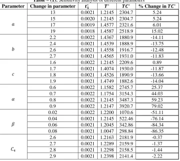
Table – (1): Sensitivity analysis of different parameters

Parameter Change in parameter 𝒕_𝟏∗ 𝑻∗ 𝑻𝑪∗ % Change in 𝑻𝑪∗

𝑎

13 0.0021 1.2145 2304.7 5.24 15 0.0020 1.2145 2304.7 5.24 17 0.0019 1.4577 2321.6 6.01 19 0.0018 1.4587 2518.9 15.02

𝑏

2.2 0.0022 1.4367 1880.9 -14.11 2.4 0.0021 1.4539 1888.9 -13.75 2.6 0.0021 1.4558 1916.7 -12.48 2.7 0.0021 1.4565 1931.0 -11.83

𝑐

1.6 0.0022 1.2145 2209.6 0.89 1.7 0.0021 1.4074 1930.0 -11.87 1.8 0.0021 1.4526 1890.9 -13.66 1.9 0.0021 1.4749 1882.6 -14.04

𝛼

0.6 0.0022 1.1582 2745.7 25.37 0.7 0.0022 1.1754 3154.3 44.03 0.8 0.0022 1.2145 3487.3 59.23 0.9 0.0022 1.2147 3920.7 79.02

𝛽

0.02 0.0022 1.2200 1070.6 -51.11 0.04 0.0021 1.2145 522.46 -76.14 0.06 0.0021 1.2045 342.86 -84.34 0.08 0.0021 1.0047 298.84 -86.35

𝐶4

2.6 0.0021 1.2163 2181.9 -0.37 2.7 0.0021 1.2289 2159.9 -1.37 2.8 0.0021 1.2298 2158.5 -1.44 2.9 0.0021 1.2398 2141.4 -2.22

On the basis of the results shown in Table 1, the following observations can be made:

• As the value of the parameters 𝑎,𝑏,𝑐 increases, 𝑇𝐶∗ and 𝑇∗ increases while 𝑡₁∗ decreases.

• As the value of the parameter 𝛼 increases 𝑇𝐶∗ and 𝑇∗ increases while 𝑡₁∗ remains the same and is insensitive to the change in 𝛼.

• As the value of the parameters 𝛽 increases,𝑇𝐶∗, 𝑇∗ and 𝑡₁∗ decreases.

• As the value of the shortage cost 𝐶₄ increases, 𝑇𝐶∗decreases and 𝑇∗ increases, while 𝑡₁∗ remains the same.

7 . CONCLUSION

In this paper the optimal total cost has been found for deteriorating items with quadratic demand. Here shortages are allowed with varying rate of backlogging. The backlogging rate is dependent on the waiting time for the next replenishment and is time proportional. The quadratic demand is best suitable for commodities which undergo seasonal variations and seems to be more realistic than exponential or linear time dependent demand. The proposed model can be extended by incorporating more features like salvage value, permissible delay in payments, quantity discounts, etc.

REFERENCES

1. Aggarwal S P, “A note on an order-level model for a system with constant rate of deterioration”, Opsearch, 15 (1978), 184-187.

2. Begum R, Sahu S K, and Sahoo R R,

Mathematical Science, 4 (2010), 271-288. 3. Begum R, Sahu S K, and Sahoo R R, “An inventory model for deteriorating items with Quadratic demand and

Partial backlogging”, British Journal of Applied Science & Technology,2(2012), 112-131.

4. Berrotoni J N, “Practical applications of Weibull distribution”, ASQC Tech. Conf. Trans., 16 (1962), 303-323. 5. Bhanu Priya Dash, Trailokyanath Singh and Hadibandhu Pattnayak, “An Inventory Model for Deteriorating

Items with Exponential Declining Demand and Time-Varying Holding Cost”, American Journal of Operations Research, 4 (2014), 1-7.

6. Biplab Karmakar and Karabi Dutta Choudhury, “Inventory models with ramp – type demand for deteriorating items with partoal backlogging and time - varying holding cost”, Yugoslav Journal of Operations Research, 24(2014), 249 -266.

© 2017, IJMA. All Rights Reserved 161

8. Covert R P and Philip G C, “An EOQ model for items with Weibull distribution deterioration,” AIIE Trans., 5 (1973), 323-326.

9. Dave U and Patel L K, “(T, Si) policy inventory model for deteriorating items with time-proportional demand”, Journal of the Operational Research Society, 32 (1989), 137-142.

10. Ghosh S K and Chaudhuri K S, “An order level inventory model for a deteriorating item with Weibull deterioration, time-quadratic demand and shortages”, Adv. Model. Optim., 6 (2004), 21–35.

11.

inventory models with Weibull distribution deterioration”, Production planning and control, 22 (2011), 437 – 444.

12. Gobinda Chandra Panda, Satyajit Sahoo and Pravat Kumar Sukla., “Analysis of Constant Deteriorating Inventory Management with Quadratic Demand Rate”, American journal of Operation Research, 2(2012), 98-103.

13. Hariga M and Benkherouf L, “Optimal and heuristic replenishment models for deteriorating items with exponential time varying demand”, European Journal of Operational Research, 79 (1994), 123-137.

14. Jagadeeswari J and Chenniappan P K, "An Order Level Inventory Model for Deteriorating Items with Time – Quadratic Demand and Partial Backlogging." Journal of Business and Management Sciences, 2.3A (2014), 17-20.

15. Jalan AK and Chaudhuri KS, “Structural properties of an inventory system with deterioration and trended demand”, International Journal of Science, 30(1999), 627-633.

16. Khanra S and Chaudhuri K S, “ A note on order level inventory model for a deteriorating item with time dependent quadratic demand”, Comput. Oper. Res., 30 (2003), 1901–1916.

17.

demand rate and partial backlogging”,

18.

2001”

19. Ouyang W U and Cheng, “An inventory model for deteriorating items with Exponential declining demand and partial backlogging”, Yugoslav Journal of Operations Research, 15(2005), 277-288.

20. Park K S, “Inventory models with partial backorders”, International Journal of Systems Science, 13 (1982), 1313-1317.

21. Philip G C, “A generalized EOQ model for items with Weibull distribution”, AIIE Transaction, 6(1974), 159-162.

22. Rangarajan K and Karthikeyan K, “Analysis of an EOQ Inventory Model for Deteriorating Items with Different Demand Rates”, Applied Mathematical Sciences, 9(2015), 2255 – 2264.

23. Sarala Pareek and Garima Sharma, “An inventory model with Weibull distribution deteriorating item with exponential declining demand and partial backlogging”, “Zenith International Journal of Multidisciplinary Research, 4 (2014), 145-154.

24. Sarkar T, Ghosh S K and Chaudhuri K S, “An optimal inventory replenishment policy for a deteriorating item with time-quadratic demand and time-dependent partial backlogging with shortages in all cycles”, Applied Mathematics and Computation, 2 (2013), 9147-9155.

25. Tripathy C K and Mishra U, “Ordering policy for Weibull deteriorating items for quadratic demand with permissible delay in payments”, Appl. Math. Sci., 4 (2010), 2181–2191.

26. Umakanta Mishra, “An EOQ Model with Time Dependent Weibull Deterioration, Quadratic Demand and

Partial Backlogging”,

545–563.

27. Vandana B K and Sharma, “An EPQ inventory model for non-instantaneous deteriorating item sunder trade credit policy”, International Journal of Mathematical Sciences and Industrial Applications, 9 (2015), 179-188. 28. Venkateswarlu R and Mohan R, “An inventory model with quadratic demand, constant deterioration and

salvage value”, Res. J. Manag. Sci., 3 (2013), 18–22.

Source of support: Nil, Conflict of interest: None Declared.