arXiv:0810.1215v1 [q-fin.ST] 7 Oct 2008
(will be inserted by the editor)
Scale free effects in world currency exchange network
A. Z. G´orski1
, S. Dro˙zd˙z1,2
, and J. Kwapie´n1
1 Institute of Nuclear Physics, Polish Academy of Science, PL–31-342 Krak´ow, Poland 2 Institute of Physics, University of Rzesz´ow, PL–35-310 Rzesz´ow, Poland
Received: date / Revised version: date
Abstract. A large collection of daily time series for 60 world currencies’ exchange rates is considered. The correlation matrices are calculated and the corresponding Minimal Spanning Tree (MST) graphs are con-structed for each of those currencies used as reference for the remaining ones. It is shown that multiplicity of the MST graphs’ nodes to a good approximation develops a power like, scale free distribution with the scaling exponent similar as for several other complex systems studied so far. Furthermore, quantitative arguments in favor of the hierarchical organization of the world currency exchange network are provided by relating the structure of the above MST graphs and their scaling exponents to those that are derived from an exactly solvable hierarchical network model. A special status of the USD during the period considered can be attributed to some departures of the MST features, when this currency (or some other tied to it) is used as reference, from characteristics typical to such a hierarchical clustering of nodes towards those that correspond to the random graphs. Even though in general the basic structure of the MST is robust with respect to changing the reference currency some trace of a systematic transition from somewhat dispersed – like the USD case – towards more compact MST topology can be observed when correlations increase.
PACS. 89.65.Gh Economics; econophysics, financial markets, business and management – 89.75.Fb Struc-tures and organization in complex systems – 05.45.Tp Time series analysis
The world currency exchange market (foreign exchange – FOREX, FX) is the world largest financial market and it constitutes an extremely complex network. The FX daily
takeover volume is of the order of 1012
USD. Any other financial market can hardly approach such volume. Also, this market has direct influence on all other markets be-cause any price is expressed in terms of a currency. The large volume makes it virtually impossible to control from outside and there is no friction (transactions are basically commission free). Due to time differences FX transactions are performed 24 hours a day, 5.5 day a week with max-imum volume between 1 and 4 p.m. GMT, when both American and European markets are open. Hence, the FX time series relations represent an exceptionally complex network indeed, and they are therefore especially worth of detailed analysis. The FX market can be viewed as a complex network of mutually interacting nodes, each node being an exchange rate of two currencies. In principle, all nodes are interconnected with complex nonlinear interac-tions. Any currency can be expressed in terms of
partic-ular one that is called the base currency. In spite of its
importance, much less attention has been paid in liter-ature to the FX cross-correlation analysis, than to such analysis of stock markets[1,2,3]. Therefore in the follow-ing the currency network will be analyzed. Our motivation to investigate correlations of FX time series is twofold: theoretical and practical. More detailed correlation
anal-ysis can give insight into the structure of links between various currencies and, in particular, it potentially may provide quantitative arguments in favor of an often postu-lated hierarchical organization of world currency exchange market. Knowledge of correlations is also essential for the portfolio management.
Usually, for a financial time series of an ithasset (i=
1, . . . , n) at time t, xi(t) =xi, one defines its return over
time period τ as Gi(t;τ) = lnxi(t+τ)−lnxi(t). For
FX series instead of a value xi(t) one has xBA(t), an
ex-change rate,i.e.a value of currencyAexpressed in terms
of a base currency B. Hence, the returns can be denoted
as GB
A(t) and they are clearly antisymmetric GBA(t;τ) =
−GA
B(t;τ). FX returns, due to the lack of commission
and high liquidity satisfy the triangle rule: GB
A(t;τ) +
GC
B(t;τ) +G A
C(t;τ) = 0 , already for relatively small
val-ues of τ[4]. As a result, for a set ofn currencies we have
N = n−1 independent values and the same number of
nodes with a given base currency.
In the following we analyze time series of daily data for 60 currencies, including gold, silver and platinum[5]. The data taken covers the time period Dec 1998–May 2005. In order to automatically get rid of possible misprints in the
original data the daily jumps greater than 5σ (less than
0.3% of data points) were removed. Also, the gaps related to non-trading days were synchronized. For each exchange rate we thus obtain a time series of 1657 data points. The
currencies are denoted according to ISO 4217 standard, and they can be formally divided into four groups, ac-cording to their liquidity. The major currencies, that we
call theA⋆ group, include USD, EUR, JPY, GBP, CHF,
CAD, AUD, NZD, SEK, NOK, DKK (11 currencies). All
other liquid currencies belong to the groupA(CYP, CZK,
HKD, HUF, IDR, ILS, ISK, KRW, MXN, MYR, PHP, PLN, SGD, SKK, THB, TRY, TWD, XAG, XAU, XPT,
ZAR, 21 currencies). Less liquid currencies (groupB)
in-clude: ARS, BGN, BRL, CLP, KWD, RON, RUB, SAR, TTD (9 currencies). Finally, the non-tradable currencies
(groupC) taken into account are: AED, COP, DZD, EGP,
FJD, GHC, HNL, INR, JMD, JOD, LBP, LKR, MAD, PEN, PKR, SDD, TND, VEB, ZMK (19 currencies). In the latter group the exchange rates are usually fixed daily by national central banks. Dividing currencies into such four groups of different liquidity is common among finance practitioners. This therefore opens an additional interest-ing issue to be verified if the different dynamics that stays behind such a division according to the liquidity (imply-ing the fix(imply-ing method) is also reflected in correlations of daily exchange rates.
For a given choice of the base currencyXthe
(symmet-ric) correlation matrix (CM) can be computed in terms of
the normalized returns, gX
A(t). To this end one takes N
time series{gX
A(t0), gAX(t0+τ), . . . , gAX(t0+ (T−1)τ)}of
length T. These series can form an N ×T rectangular
matrix MX, and the CM can be written in the matrix
notation as
CX≡[CX]AB = 1
T M
XMfX , (1)
where tilde stands for the matrix transposition. By con-struction the trace of the CM is equal to the number of
time series Tr CX = N. When some of the time series
become strongly dependent, the related number of
eigen-values approach value zero (zero modes). This effect,
typi-cal for FX data, does not occur for the stock market time series.
Sample spectra of CMs for the same time series as the ones considered here, using several different base
curren-cies X, can be found in [6]. In all the cases one finds a
maximal eigenvalue (λmax, in our case max =N = 59)
that is well separated from all the remaining eigenvalues
and is placed within the range 0.2N÷0.9N, with average
around 0.5N. With a few exceptions, there are also clearly
isolated second maximal eigenvalues (λmax−1),
consider-ably smaller thanλmax, but also well separated from the
bulk of other eigenvalues. At the same time, the mag-nitude of the largest eigenvalue significantly depends on
which currency is used as a baseX. The largest maximal
eigenvalues correspond to those base currencies that either have a very strong drift, independent of the behavior of other currencies (like GHC) or whose fluctuations are to a large extent independent of the global FX behavior. The
smallest values of λmax appear when the USD or other
currencies that are strongly tied to it are used asX. This
reflects the fact that changes in value of the USD - due to its global world significance - cause a rich diversity of reactions of all other currencies. In other words, their
dy-namics viewed from the USD perspective looks less coop-erative as compared to the cases when the base currency is not that influential. Thus, effectively eliminating the USD by using it as the base currency sizeably diminishes cor-relations among all other currencies. Another interesting manifestation of this effect will be seen in the Minimal Spanning Tree (MST) graphs picture. It should be men-tioned that analogous characteristics for eigenvalues have been identified in the smaller subsectors (like tradable and non-tradable separately) of the analyzed currencies.
The structure of eigenspectrum is one way to get in-sight into large amount of data as represented by the cor-relation matrices. A complementary - efficient and con-clusive - way to visualize such ensembles of data is in terms of the MST graphs. In the following we use the MST graphs approach in order to further explore prop-erties of the currency exchange network. The MST was introduced in graph theory quite long ago [7,8]. Later it was rediscovered several times [9,10]. To analyze the stock market correlations it was applied by Mantegna [11] and later on by several authors [12,13,16,17]. Recently MST graphs were used to study FX correlations[18,19,20]. Here we present the most exhaustive results concerning the FX data, for 60 world currencies.
To construct the MST graph we choose the following measure
dX(A, B) =q(1
−CX
AB)/2, d
X(A, B)
∈[0,1], (2) that satisfies the standard axioms of metric. The distance
dbetween two time series is smaller if their correlation
co-efficient is closer to unity. One node (vertex) in the graph corresponds to each time series. We shall connect the two
nodes,AandB, with a line (edge, “leg”), ifd(A, B) is the
smallest. In the next step we look for another two closest nodes and again we connect them with a line. This proce-dure is repeated until we obtain a connected tree graph.
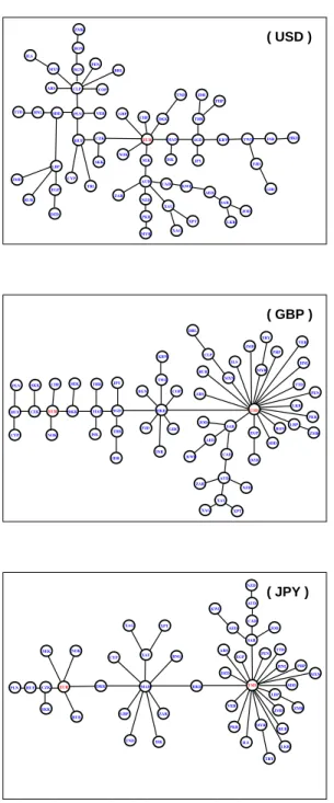
We callmultiplicity(degree) of that node the number
of legs attached to it. Clearly, multiplicity of a node is an
integer number,K. In our case we haveN = 59 nodes for
a given base currency. As examples, Fig. 1 shows the MST graphs for our set of data for three major currencies, USD,
GBP and JPY, taken as the base currency. For a nodeA
its multiplicity is denoted by KA. Integer N′(K) is the
number of nodes with exactly K legs. Because the total
number of nodes,N, is relatively small, we introduce the
integrated quantity
F(K) =N(K)/N= 1
N
KXmax
I=K
N′(I), (3)
where Kmax denotes the maximal number of legs in the
MST graph.N(K) is the number of nodes withKor more
legs. Counting legs in all nodes of our MST graph we can
construct discrete functionN(K) and its normalized
ver-sion,F(K).
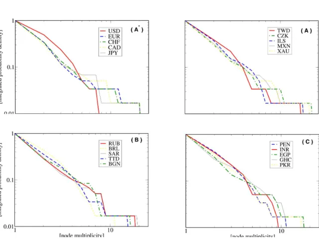
In Fig. 2 we show theF(K) plots for the MST node’s
multiplicity for different base currencies from each of the
DZD EGP LBP RUB JMD SDD HNL TTD PLN HUF CYP TRL CZK SKK VEB EUR
ARS CLP COP
BRL PEN BGN RON ZMK MXN ILS GBP CHF DKK TND SEK AUD ZAR NZD PKR MYR CAD XAU XAG XPT KWD AED SAR LKR JOD MAD ISK JPY SGD THB IDR PHP
KRW TWD INR HKD
NOK
FJD
GHC
( USD )
EGP DZD SAR SDD RON LBP ZMK PKR LKR PEN TTD HNL VEB PHP MYR TRY JMD ILS MXN ARS RUB CLP BRL JOD AED CAD AUD NZD XPT USD XAU ZAR XAG KWD HKD COP GHC TWD KRW INR FJD BGN SGD THB IDR JPY MAD THD ISK DKK SEK EUR NOK CHF SKK CZK HUF PLN CYP
( GBP )
USD LBP SDD MXN PHP HNL ZMK JMD RUB LKR TRY MYR ILS VEB PKR PLN DZD EGP SAR JOD PEN TTD CAD AUD NZD KWD AED ARS HKD
HUF CZK EUR DKK MAD
ZAR GBP TND ISK BNG XPT XAG XAU CYP NOK SEK SKK RUB
( JPY )
Fig. 1. MST graphs for all the currencies taking USD, GBP and JPY as the base currency, respectively.
we present the distributions for five typical basic curren-cies from each group. Already at first glimpse, basically all plots indicate scaling and their similarity extends even to a quantitative level. One subtle difference can be visible when the USD (as well as the other currencies linked to it) is used as reference. Here, in the log-log scale one observes a somewhat faster decrease than linear. Nevertheless, fit-ting it with the straight line results thus in a steeper slope and the worse quality of such a fit. The relevant detailed
numerical parameters, including the power exponent α,
its standard error (∆α), and values of the maximal CM
eigenvalues, for all the 60 currencies used as the base for the remaining ones are listed in Tables 1-4. The exponents
Table 1. Characteristics of the power fits for the MST node’s multiplicity of all the currencies using the base currencies from the groupA∗.
base currency α ∆α ∆α/α λmax
AUD 1.43 0.08 5.4% 32.1
CAD 1.39 0.11 7.7% 23.2
CHF 1.34 0.08 6.0% 29.9
DKK 1.33 0.08 5.9% 27.4
EUR 1.30 0.08 5.9% 27.6
GBP 1.44 0.11 7.6% 24.1
JPY 1.36 0.08 6.0% 32.6
NOK 1.41 0.08 5.5% 28.4
NZD 1.43 0.07 5.0% 34.4
SEK 1.41 0.07 4.7% 29.2
USD 1.92 0.18 9.6% 11.8
average 1.43 0.09 6.3% 27.3
Table 2. Characteristics of the power fits for the MST node’s multiplicity of all the currencies using the base currencies from the groupA.
base currency α ∆α ∆α/α λmax
CYP 1.42 0.07 4.6% 36.6
CZK 1.33 0.08 5.8% 31.7
HKD 2.31 0.32 14.0% 11.7
HUF 1.38 0.08 5.8% 31.8
IDR 1.48 0.09 5.9% 43.7
ILS 1.56 0.12 7.9% 24.2
ISK 1.47 0.09 5.9% 27.6
KRW 1.59 0.11 6.7% 27.8
MXN 1.51 0.07 4.3% 29.8
MYR 2.25 0.31 14.0% 11.9
PHP 1.62 0.11 6.7% 24.5
PLN 1.49 0.08 5.7% 32.0
SGD 1.67 0.10 5.9% 13.8
SKK 1.41 0.06 4.4% 31.7
THB 1.50 0.11 7.3% 20.5
TRY 1.55 0.08 5.1% 43.3
TWD 1.61 0.12 7.7% 15.2
XAG 1.48 0.11 7.7% 46.7
XAU 1.38 0.08 5.5% 37.2
XPT 1.40 0.09 6.3% 47.1
ZAR 1.50 0.08 5.7% 41.8
average 1.57 0.11 6.8% 30.0
αand their standard errors∆αwere determined with the
least square fit of corresponding power functions in the original linear scale. Because the total number of data points equals 59 and the number of occupied bins is typ-ically around 10 more sophisticated statistical estimates do not seem adequate in this case.
It can be concluded that the scale free behavior and thus the power like fit are fairly good for majority of the
base currencies. The worst scaling (if at all),∆α/α≥9%,
was obtained for the USD and currencies tied to it (HKD, MYR, LBP). A technical reason for the latter effect is, that taking USD as the base currency one eliminates its
Fig. 2.Log-log plots of the functionF(K) for five sample base currencies taken from each group:A∗,A,BandC, respectively.
Table 3. Characteristics of the power fits for the MST node’s multiplicity of all the currencies using the basic currencies from the groupB.
base currency α ∆α ∆α/α λmax
AED 1.92 0.13 6.5% 17.5
ARS 1.45 0.06 4.4% 40.2
BGN 1.44 0.09 5.3% 32.3
BRL 1.60 0.11 6.7% 43.5
CLP 1.48 0.09 6.0% 31.0
KWD 1.85 0.11 6.1% 17.9
RON 1.50 0.08 5.0% 36.7
RUB 1.48 0.09 5.8% 44.5
SAR 1.65 0.09 5.3% 16.9
TTD 1.97 0.14 7.1% 15.6
average 1.63 0.09 5.8% 29.6
node from the MST graph. Hence, the largest cluster (i.e. large multiplicity node) disappears, the tail of the distri-bution is getting thinner and the MST graph is too small to be able to reproduce fat tails (i.e. power like distri-bution). On a more fundamental level, this characteristic feature associated with the USD – as seen from the MST perspective – may reflect its special status in the world economy during the period considered here. It is proba-bly also worth to notice that the quality of scaling goes
Table 4. Characteristics of the power fits for the MST node’s multiplicity of all the currencies using the base currencies from the groupC.
base currency α ∆α ∆α/α λmax
COP 1.46 0.07 7.1% 30.8
DZD 1.44 0.08 6.3% 51.3
EGP 1.50 0.32 4.7% 39.5
FJD 1.48 0.08 6.0% 31.0
GHC 1.54 0.09 4.9% 52.2
HNL 1.81 0.12 5.0% 14.0
INR 1.92 0.09 5.5% 14.3
JMD 1.66 0.09 9.0% 35.0
JOD 1.80 0.07 5.5% 20.6
LBP 1.31 0.31 9.0% 24.6
LKR 1.73 0.11 7.3% 18.5
MAD 1.37 0.08 11.0% 21.1
PEN 1.78 0.10 7.5% 17.4
PKR 1.70 0.06 4.7% 25.1
SDD 1.67 0.11 5.8% 25.8
TND 1.39 0.08 8.0% 21.6
VEB 1.44 0.12 5.8% 37.6
ZMK 1.31 0.11 7.7% 49.3
somewhat in parallel with the magnitude of the largest eigenvalue (last column in the Tables) of the original cor-relation matrix. The disputable – as far as the scaling is concerned – cases are typically associated with the
rela-tively small magnitudes of λmax and thus with the lower
degree of collectivity.
For the prevailing majority of the base currencies the statistical significance of the scaling effects is however quite convincing. Even more, the corresponding scaling expo-nents do not differ much among the four groups of curren-cies considered. The scale free behavior of MST graphs is in agreement with the successful usage of hierarchi-cal structure methods in finance [20] and the fat tails are signature of currency clustering in MST graphs. In more quantitative terms, the power like scaling of nodes’ degree has been shown in hierarchical networks [21,22] and the corresponding scaling exponents derived analytically. In the context of our present study it is very interesting and encouraging to find out that the average value we have
obtained for the tail index ishαi= 1.55 while the
hierar-chical model discussed in [21,22] implies very close value (for the cumulative distribution)
αhier = lnM/ln(M −1) = 1.61. (4)
The replication factor M to be used in this formula in
our case can be calculated from the average node degree:
M = hKi+ 1 = 2(N −1)/N + 1 = 2.966. The scaling
exponent (4) thus differs from our average value hαi by
less than 4%. This fact provides a significant quantitative argument in favor of the hierarchical organization of the world currency exchange market, an effect which already can visually be inferred from the panels corresponding to GBP and JPY in Fig. 1.
The panel corresponding to the USD looks less explicit in this respect. Indeed the quality of the corresponding scaling is here not so convincing. Nevertheless,
approxi-mation with the power like fit gives the exponentαwhich
is significantly larger (Table 1) than in the above hierar-chical model. In fact, the node’s multiplicity distribution corresponding to this case and seen in Fig 1, develops some departure towards a Gaussian distribution and thus indi-cates some admixture of randomness and a more ”demo-cratic” multiplicity distribution as compared to a pure hi-erarchical situation. This effect also is consistent – as
ex-pressed by the correspondingλmax in Table 1 – with the
weakest synchronization of the currency exchange rates expressed in the USD. Interestingly, a correspondence of this kind seems to be leaving imprints for the other cur-rencies when they are used as reference for all remaining. As it can be seen from Tables 1-4 the smaller values of
λmax (and thus weaker correlations) are quite
systemat-ically associated with the scaling exponents α which are
larger than their average valuehαi= 1.55 while the larger
values ofλmax(stronger correlations) are typically
associ-ated withαsmaller than this average. For a better
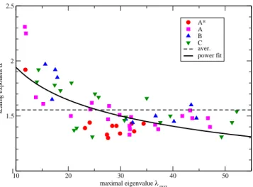
visu-alization the quality of such a tendency is demonstrated
in Fig. 3 by the scatter plot of α versus the
correspond-ing λmax for all the 60 currencies. An overall decrease
of αwith increasingλmax is quite evident from this
Fig-ure. It is faster in the region of smaller λmax values and
10 20 30 40 50 maximal eigenvalue λ max
1 1.5 2 2.5
scaling exponent
α
A* A B C aver. power fit
Fig. 3.Scatter plot ofαversusλmaxfor all the 60 currencies.
Four different symbols correspond to four different groups of the currencies as described in the inset. The solid line repre-sents the best fit in terms of a power function and the dashed horizontal line indicates the averagehαi.
then tends to saturation. The best simple representation for this dependence (solid line in Fig. 3) is in terms of a
power function (α∼(λmax−λmaxRM)−β) withβ≈0.21. As
λRM
maxthe upper bound of the Wishart ensamble of random
matrices is used. Thus λRM
max= 1 + 1/Q+ 2/
√
Q[14,15],
where Q=T /N which in our case givesλRM
max= 1.413.
The above correspondence between λmax and α
re-mains in accord and in fact constitutes an extension of the observation made in ref. [16] in connection with the stock market. There it is shown that the MST scaling ex-ponent evaluated during crash periods – whose dynamics is inherently associated with stronger correlations [23] – is smaller than during normal business periods. As already mentioned and even more extensively discussed in [6] the currencies exchange rates expressed in terms of a less in-fluential currency are more correlated as compared to the situation when the leading ones are used as reference. It is also interesting to see that the above coincidences apply to all the four groups of currencies listed in Tables 1-4 and displayed in Fig. 3 (where they are seen to overlap with each other) even though they are characterized by size-ably different liquidity and in some cases (group C) even by non-trade mechanism of setting the exchange rates. This implies that the general characteristics of the cor-responding MST’s are quite robust with respect to such factors.
The power like behavior with the scaling exponent
α = 1.6, which is very close to the one estimated in
the present study, was also found [13] for the stock mar-ket MST graphs. Furthermore, similar characteristics have been identified in several other natural and artificial com-plex networks studied so far in the literature – for refer-ences see [24,25] – and the world currency network con-sidered here belongs to this universality class, with the
References
1. L. Laloux, P. Cizeau, J.-P. Bouchaud, M. Potter, Phys. Rev. Lett.831467 (1999).
2. V. Plerou, P. Gopikrishnan, B. Rosenow, L. A. N. Amaral, H. E. Stanley, Phys. Rev. Lett.831471 (1999).
3. J. Kwapie´n, S. Dro˙zd˙z P. O´swi¸ecimka, Physica A 359589 (2006).
4. Y. Aiba, N. Hatano, H. Takayasu, K. Marumo, T. Shimizu, Physica A324253 (2003).
5. Sauder School of Business, Pacific Exchange Rate System, http://fx.sauder.ubc.ca/data.html (2006).
6. S. Dro˙zd˙z, A. Z. G´orski, J. Kwapie´n, Eur. Phys. J. B 58
499 (2007).
7. The algorithm to construct MST graphs was for the first time published by Czech mathematician, Otakar Bor ˙uvka in 1926.
8. J. Kruskal, Proc. Am. Math. Soc.748 (1956).
9. C.H. Papadimitrou, K. Steigliz, Combinatorial Optimiza-tion, (Prentice-Hall, Englewood Cliffs 1982).
10. D.B. West, Introduction to Graph Theory (Prentice-Hall, Englewood Cliffs 1996).
11. R. N. Mantegna, Eur. Phys. J. B11193 (1999).
12. J.-P. Onella, A. Chakraborti, K. Kaski, J. Kert´esz, Physica A324247 (2003).
13. G. Bonanno, G. Caldarelli, F. Lillo, R. N. Mantegna, Phys. Rev. E68046130-1 (2003).
14. V. A. Marchenko, L. A. Pastur, Mat. Sb.72507 (1967). 15. A.M. Sengupta, P.P. Mitra, Phys. Rev. E603389 (1999). 16. J.-P. Onella, A. Chakraborti, K. Kaski, J. Kert´esz, A.
Kanto, Phys. Rev. E68056110-1 (2003).
17. G. Bonanno, G. Caldarelli, F. Lillo, S. Miccich`e, N. Van-dewalle, R. N. Mantegna, Eur. Phys. J. B38363 (2004). 18. M. McDonald, O. Suleman, S. Williams, S. Howison, N. F.
Johnson, Phys. Rev. E72046106 (2005).
19. A. Z. G´orski, S. Dro˙zd˙z, J. Kwapie´n, P. O´swi¸ecimka, Acta Phys. Pol. B372987 (2006).
20. M. J. Naylor, L. C. Rose, B. J. Moyle, Physica A382199 (2007).
21. E. Ravasz, A.-L. Barab´asi, Phys. Rev. E67026112 (2003). 22. J. D. Noh, Phys. Rev. E67045103(R) (2003).
23. S. Dro˙zd˙z, F. Gr¨ummer, A. Z. G´orski, F. Ruf, J. Speth, Physica A2874400 (2000).
24. R. Albert, A.-L. Barab´asi, Rev. Mod. Phys7447 (2002). 25. S. Boccaletti, V. Latora, Y. Moreno, M. Chavez, D.-U.