Ridesharing: Simulator, Benchmark, and Evaluation

(1)

Ridesharing: Simulator, Benchmark, and Evaluation

James J. Pan

Tsinghua University, China

[email protected]

Guoliang Li

Tsinghua University, China

[email protected]

Juntao Hu

Beihang University, China

[email protected]

ABSTRACT

Ridesharing is becoming a popular mode of transportation with profound effects on the industry. Recent algorithms for vehicle-to-customer matching have been developed; yet cross-study evaluations of their performance and applicabil-ity to real-world ridesharing are lacking. Evaluation is com-plicated by the online and real-time nature of the rideshar-ing problem. In this paper, we develop a simulator for evaluating ridesharing algorithms, and we provide a set of benchmarks to test a wide range of scenarios encountered in the real world. These scenarios include different road networks, different numbers of vehicles, larger scales of cus-tomer requests, and others. We apply the benchmarks to several state-of-the-art search and join based ridesharing al-gorithms to demonstrate the usefulness of the simulator and the benchmarks. We find quickly-computable heuristics out-performing other more complex methods, primarily due to faster computation speed. Our work points the direction for designing and evaluating future ridesharing algorithms. PVLDB Reference Format:

James J. Pan, Guoliang Li, Juntao Hu. Ridesharing: Simula-tor, Benchmark, and Experimental Evaluation. PVLDB, 12(10): 1085–1098, 2019.

DOI: https://doi.org/10.14778/3339490.3339493

1. INTRODUCTION

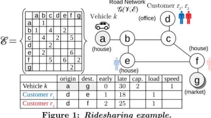
Ridesharing is an emerging mode of transportation cur-rently having a deep impact on the personal transportion industry. The basic concept is that customer passengers needing transport can hail participating vehicles on their smartphones. These vehicles can serve multiple passengers at a time in order to take advantage of similar trips to save travel distance and fuel cost. Figure 1 gives an example.

Commercial services today are already facing enormous customer loads, on the order of millions per day [2]. Soci-etal benefits from ridesharing [40, 10, 24] can be captured by optimizing assignment of customers to vehicles so as to max-imize utilization of the vehicles while simultaneously using

This work is licensed under the Creative Commons Attribution-NonCommercial-NoDerivatives 4.0 International License. To view a copy of this license, visit http://creativecommons.org/licenses/by-nc-nd/4.0/. For any use beyond those covered by this license, obtain permission by emailing [email protected]. Copyright is held by the owner/author(s). Publication rights licensed to the VLDB Endowment.

Proceedings of the VLDB Endowment,Vol. 12, No. 10 ISSN 2150-8097.

DOI: https://doi.org/10.14778/3339490.3339493

least possible travel distance. These assignment decisions can be characterized by the speed of the decision-making al-gorithm and the quality of the assignment toward optimiza-tion objectives. Despite studies on assignment approaches from the database [11, 12, 41, 36, 37, 9, 27, 20] and other communities [6, 29, 22, 16, 34, 5, 15], challenges remain.

First, most evaluations do not consider the online and real-time nature of ridesharing, possibly because offline eval-uation is much simpler. But these offline evaleval-uations do not reflect the real world. Thus, there is a need for an online and real-timeevaluation platform.

Second, there is no consistent benchmark for ridesharing, needed due to huge variation in problem scenarios. Algo-rithm performance can be affected by many factors: the road network; volume and velocity of customer and vehi-cle streams; properties of the customers and vehivehi-cles, in-cluding their distribution throughout the network; and so on. A benchmark would standardize these factors and pro-vide guidance for algorithm design. Existing benchmarks for the related Dial-A-Ride problem (DARP) [15] cannot be adapted because (1) DARP does not consider road net-works; (2) the customers and vehicles do not represent real ridesharing scenarios; and (3) the datasets are small com-pared to ridesharing instances [28, 30, 19]. Thus separate benchmarks for ridesharing are needed.

Third, cross-study evaluations of algorithms from inde-pendent studies with precise analysis of strengths and weak-nesses are currently missing, difficult due to the complex nature of the ridesharing problem. For example, evaluation procedures must address how to handle real-timematch la-tency; they must also measure total travel distance of the vehicles over the period of a scenario, crucial for compar-ing algorithm quality. In terms of techniques, the database community has focused on filtering, data structures, and heuristics to achieve algorithm speed while others have em-phasized grouping and other procedures for improving qual-ity. A standardized evaluation of these different approaches is necessary for understanding their merits, drawbacks, and applicability to real-world ridesharing problems.

To fill these gaps, we make the following contributions: (1) We develop the Cargo system for implementing and eval-uating ridesharing algorithms through online, real-time sim-ulation. Our system provides standard components and rou-tines to ease implementation, and offers a single evaluation protocol for ridesharing events (vehicle motion, assignment events, etc.) that can be used to objectively compare

dif-1

(2)

a b c d e f g a 1 b1 4 2 c 4 2 5 d 2 e 2 6 f 5 6 2 g 2

ℰ

=

origin dest. early late cap. load speed

Vehicle k a g 0 30 2 1 Customer r₁ d e 1 18 1 Customer r₂ d f 2 25 1 Customer r1, r2

a

d

(house) (house) (house) (market) (office)

c

b

e

f

g

🚗

🚹

Road Network 𝒢(𝒱,ℰ)

🚹

Vehicle k

Figure 1: Ridesharing example.

ferent algorithms. Our system is open source, available to practitioners for conducting online experiments [1]. (2) We present a set of benchmark instances for the stan-dardized evaluation of algorithms. Our benchmark is de-signed based on real road networks with different features (e.g. sizes and geometries) and on real ridesharing customers and vehicles. The benchmark allows us to manipulate prop-erties of the problem to test different situations.

(3) We present an experimental comparison of recent rep-resentative algorithms using our benchmark and system, and we report comprehensive findings from our experimental evaluation. We provide new insights on the strengths and weaknesses of existing algorithms that can guide practition-ers to select appropriate algorithms for various scenarios.

The rest of this paper is organized as follows. Section 2 defines the ridesharing problem. Section 3 describes the algorithms we evaluated. Section 4 describes the Cargo sys-tem. Section 5 describes the benchmarks used in this paper. Section 6 presents experimental results and our analysis. Fi-nally, Section 7 concludes our work.

2. BACKGROUND

2.1 Preliminaries

Table 1 summarizes our notation.

Road Network. Let a directed graphG(V,E) represent a road network, with nodes inV representing intersections and edges inE representing streets. Each edge (u, v) ∈E has a weightwuv (e.g. travel distance along the street). A route is another name for a path throughG, and its cost is the sum of the weights of all the edges in the path.

Vehicles and Customers. Let vehicles and customers be

represented by origin-destination pairs. For simplification, assume that these are bound to nodes inV. If an origin or destination is not exactly at a node, it can be mapped to the nearest node using existing methods [42].

Each vehiclekbegins atransportation serviceat its origin ko and ends the service at its destinationkd. It moves by following a route from ko to kd with a certain speed. Its earliest possible departure time from ko (early time) and its latest acceptable arrival time atkd(late time) form the vehicle’stime window [ek, lk], whereek< lk.

Each customerrbegins at its originro and requests to be transported to its destinationrdby traveling with a vehicle that is in service. The assigned vehicle will move toro to pick up the customer, then tordto drop off the customer, thereby satisfying the customer’s travel request. Each cus-tomer also has a time window [er, lr]. The early time er gives the earliest possible time a vehicle can pick up cus-tomerr, and the late timelr gives the latest drop off time that the customer can accept. Note that time windows on the vehicles and customers generalize “maximum detour” and similar service guarantees encountered in the real world.

Table 1: Notation used in this paper.

Notation Description

n, m Number of customers, vehicles r∈N, k∈M Set of customers, vehicles ro, rd Customer origin, destination

ko, kd Vehicle origin, destination

ek, er Early time for vehiclek, customerr

lk, lr Late time for vehiclek, customerr

Qk, qr Capacity of vehiclek, load on customerr

kgps Current location of vehiclek ud(u, v) Euclidean distance fromutov cuv Shortest-path cost fromutov

S={u1, . . . , us} Schedule with lengths

C(S, k) Cost of scheduleStaken by vehiclek

Each vehiclek has an initial capacityQk >0, and each customerris associated with a loadqr>0. When a vehicle picks up customerr, its capacity decreases byqr; when the vehicle drops offr, its capacity increases byqr.

Example 1. We use Figure 1 as a running example. The edgesE of the road network are given in the adjacency ma-trix; the nodes are V = {a, b, c, d, e, f, g}. Vehicle k has origin at nodea, destination at nodeg, and moves 1 unit of distance per unit of time. Customerr1 aims to travel from d to e, and customer r2 aims to travel from d to f. The bottom table shows time windows, capacities, and loads.

2.2 Ridesharing Problem (RSP)

Given vehicles and customers on a road network, the goal of the Ridesharing Problem (RSP) is to find the minimum-cost set of vehicle routes that can serve all customers, sub-ject to the following constraints:

• Precedence. A vehicle must visitro first, and thenrd, in order to serve customerr.

• Time Windows. Each vehicle k must depart fromko and arrive atkd within the time window [ek, lk]. For each customerr that it serves, it must serve the cus-tomer within the time window [er, lr].

• Capacities. Each vehicle’s capacity must always be positive or zero.

Example 2. In the example, the solution is to route vehi-clekthrough the node sequence{a, b, c, d, c, b, e, f, g}, serv-ing both customers. This route has a cost of 23. If k, r1, and r2 traveled individually (no ridesharing), the sum of their individual costs is 27.

Online Assignment. In the online problem, vehicles and

customers are not known beforehand, but revealed through-out the day at their early times. Each revealed customer must be assigned to a vehicle that is in service, and then the route for that vehicle must be adjusted in order for it to serve the customer. The objective is to minimize the total route cost across all the vehicles at the end of the day.

As vehicles are given new assignments, their routes can change. For each vehicle, its final route cost after it has ended service is used to compute the total route cost.

Optimization Goals. As not every customer can be

fea-sibly served in the real world due to tight time windows, some studies relax the requirement to serve all customers, then add a penalty on the total route length for the un-matched customers [38, 6, 22, 34]. Others formulate the online problem as a series of offline instances, and then aim to optimize each of the instances [27, 20, 14, 41], while others simplify the problem to one-to-one matching where vehicles have only one capacity [36, 29, 9, 5]. Other studies use profit maximization as the objective [41]. Some studies do not aim at global optimization, instead offering customers choices based on price and time [11, 12, 9].

(3)

Vehicle Schedule.Given a customer request, we first need to find a valid vehicle for the customer, which is one where there exists at least one route for the vehicle to serve the customer while satisfying all the constraints. We then adjust the route of the vehicle.

The minimum-cost route for a vehicle can be expressed using the vehicle’s schedule. Let scheduleS ={u1, . . . , us} be an ordered sequence of s unique customer origins and destinations ui, where 1 ≤i≤ s gives the position of the origin or destination in the schedule. Each arrangement of the elements produces a different schedule. By following a particular schedule, vehiclek visits each of the origins and destinations in given order while it travels from ko to kd. The shortest route through this schedule is formed by the shortest paths through each of the schedule’s elements. Let cuvbe the shortest path cost from nodeuto nodev. Then,

C(S, k) =cko,u1+ s−1 X

i

cui,ui+1+cus,kd (1)

expresses the cost of scheduleSbased on the shortest route for vehicle k. The minimum-cost route for k thus corre-sponds to the least-cost permutation ofS using Equation 1.

Example 3. The best schedule for vehiclekin the example is{a, d, d, e, f, g}, with costcad+cdd+cde+cef+cf g= 23.

Problem Complexity. If all vehicles have their origin

and destination at a single common depot, then the RSP is equivalent to the DARP. The DARP is known to be NP-hard because it generalizes the Traveling Salesman Problem [15]. Having multiple vehicle origins and destinations does not lose generality, thus the RSP is NP-hard.

Relation to Ridehailing.We make the following

distinc-tion. Ridehailing vehicles, as opposed to ridesharing ve-hicles, have no late windows and no destinations of their own. These “taxis” can be modeled in the RSP by giving them infinite late windows and some imaginary destination. Ridesharing is clearly more general. In preliminary tests, we found that taxis can double the number of matches over ridesharing vehicles because they can continually serve re-quests. Hence, all our benchmarks in Section 5 use taxis.

2.3 Related Work

DARP Benchmarks. Many benchmarks exist for the

DARP [28, 30, 19], but they cannot be adapted to the RSP as discussed in Section 1. First, the RSP and DARP operate on different graphs. In the DARP, the graph is complete and forncustomers there are totally 2n+ 2 nodes. These nodes represent all customer pickups and dropoffs, and include two extra nodes for an “origin depot” and “destination depot”. A weighted edge exists for each node pair. All weights are given and can represent distance, time, or some other met-ric. Each vehicle route (path through the graph) must begin from the origin depot and end at the destination depot. In the RSP, the graph is not complete. Each node maps to a physical location on a road network. A path through this graph corresponds to a physical route through the road net-work. The number of nodes depends on the size of the road network and the mapping method. An edge exists between a pair of nodes only if there is a physical road segment that connects them without passing through other nodes. Edge weights represent distance and can be converted to time if the travel speed along the road segment is known.

Second, the RSP is online in practice. DARP requests are usually known in advance [15] whereas RSP requests ar-rive continuously throughout the day. Some DARP methods may be used on the RSP, but they must be adapted for road networks and for the online scenario. To our knowledge, two DARP methods have presently been tried on the RSP. We point them out in Section 3.

Comparison Studies. Some small-scale comparison

stud-ies exist. One study compares three RSP strategstud-ies on a simulation of the Seoul road network [22] using 600 vehicles and a customer request rate of around 1.3 requests per sec-ond. Another study [14] uses up to 500 vehicles and a rate of around 5.6 requests per second on simulations of the New York City and Chicago road networks. Our evaluation in Section 6 adds to existing comparison studies by evaluating more algorithms and at real-world scale.

Experimental Platforms. Some platforms exist for

test-ing logistics and other road network problems. In [4], a sim-ulator is presented that can model millions of agents over a large range of mobility decisions. Similarly, in [23] a traffic simulator is presented to investigate vehicle routing choices. In [39], a specialized platform is designed to test algorithms for pickup-and-delivery problems, and in [8], a platform for generating moving objects on a road network is introduced. With modification, some of these platforms may support evaluating RSP algorithms. Our platform is designed specif-ically for ridesharing by including components and routines common to ridesharing algorithms.

3. RIDESHARING ALGORITHMS

In this section, we discuss an exact algorithm for the of-fline problem and several online algorithms. We present our evaluations on all algorithms in Section 6 using the system and benchmarks described later.

3.1 Branch-and-Bound

Branch-and-Bound (BB) [26] is a general technique for solving mixed-integer linear programs. It has been used for the DARP [15] and can be directly applied to the offline RSP. The RSP can be formalized as an integer minimization program in order to use BB.

Formalization. An integer-based labeling scheme is used

to formulate the program. Letmbe the number of vehicles and n the number of customers. Now the vehicles can be labeled from 1 to m, and the customers from 1 to n, to form two sets of integer labelsMandN, respectively. Using

these sets, the origins and destinations of the customers and vehicles can be labeled. For each vehicle with labelkwhere k∈M, its origin can also be labeledk, and its destination

can be labeledm+k. All the vehicle origin labels thus form the setMo={1. . . m}, and all the vehicle destination labels form the set Md = {m+ 1. . .2m}. In a similar manner, for each customer with label r wherer ∈N, its origin and

destination can be labeled to produce the set of all customer origin labels No = {2m+ 1. . .2m+n}and the set of all customer destination labelsNd={2m+n+ 1. . .2m+ 2n}. Now, the RSP is formalized as the optimization problem

Minimize X k∈M X i∈V X j∈V cijxkij, i6=j (2) whereV =No∪Nd∪ {k, k+m}is the union of all possible origins and destinations that vehicle k can visit,cij is the shortest-path cost from the stops represented by i and j, and xkij is a binary decision variable equal to 1 ifk travels from stopidirectly to stopjin its route, and 0 otherwise.

(4)

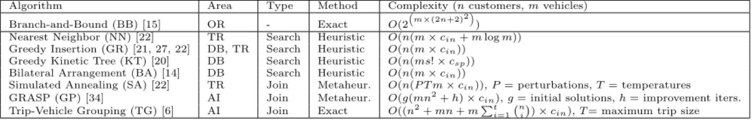
Table 2: Ridesharing algorithms. Complexity is written in terms of the customer insertion costcin. For simple insertion, cin =O(s3×csp) where s is schedule length and csp is the cost of finding one shortest path. Areas: OR=Operations Research; DB=Database; TR=Transportation; AI=Artificial Intelligence.

Algorithm Area Type Method Complexity (ncustomers,mvehicles) Branch-and-Bound (BB) [15] OR - Exact O(2

m×(2n+2)2

) Nearest Neighbor (NN) [22] TR Search Heuristic O(n(m×cin+mlogm))

Greedy Insertion (GR) [21, 27, 22] DB, TR Search Heuristic O(n(m×cin))

Greedy Kinetic Tree (KT) [20] DB Search Heuristic O(n(ms!×csp))

Bilateral Arrangement (BA) [14] DB Search Heuristic O(n(m×cin))

Simulated Annealing (SA) [22] TR Join Metaheur. O(n(P T m×cin)),P= perturbations,T= temperatures

GRASP (GP) [34] AI Join Metaheur. O(g(mn2₊_h₎_×_c

in),g= initial solutions,h= improvement iters.

Trip-Vehicle Grouping (TG) [6] AI Join Exact O((n2₊_mn₊_mPt i=1

n i ₎

×cin),T= maximum trip size Constraints. Equation 2 is subject to constraints on the

routes (Section 2.2) including that each served customer must be served by the same vehicle, and that each vehi-cle must begin at its origin and end at its destination. The labeling scheme allows these constraints to be generally ex-pressible, as demonstrated in [15].

Branch-and-Bound. A search tree is used to explore

so-lutions to the above formalization. The search tree works by listing solutions to “relaxed” problems, where the integer constraint on thexkijvariables is removed (but they are still bounded by 0 and 1). Each node in the tree represents one such solution, and different solutions are obtained by fixing certain variables to be 0 or 1 for specific values ofi, jandk. Each node has a cost equal to the value of the solution given by Equation 2. The tree is searched as it is constructed.

To initialize the tree, the root node is constructed by solv-ing the relaxed problem, where 0≤xkij≤1 for alli, j, and k, using simplex [32] or other methods. The cost of this so-lution establishes the lower bound on the minimum cost by nature of being optimal. If this solution is already integer (all variables are integer), it is the optimal solution to the original problem and we are done. Otherwise, the rest of the tree is iteratively searched and constructed as follows.

(1) Branch. Create two child nodes for every node that represents a non-integer solution (in the first iteration, there is only the root node). Each child takes the same relaxed problem as its parent, except randomly select specific values fori, jandkand setxk

ij:= 0 for one child, andxkij:= 1 for the other. Now both child nodes represent two new relaxed problems, each with one less binary variable.

(2) Bound. Solve each new relaxed problem to obtain new solutions. For each new solution:

• If the solution is non-integer and there is no current upper bound or its cost is below the bound, take its cost to be the new upper bound, and then follow (1) to branch the node; otherwise prune the node. • If the solution is integer, then if there is no current

incumbent solution, or if its cost beats the current in-cumbent, it becomes the new incumbent and no longer needs to be branched; otherwise, prune the node. When no more nodes are left to be branched, then the final incumbent is the optimal integer solution.

The worst-case complexity of Branch-and-Bound is expo-nential. In this case, all nodes are feasible and no nodes are pruned. There arem(2n+ 2)2 _{binary variables} (num-ber of vehicles multiplied num(num-ber of i, j pairs), each with two possible values; hence the complexity isO(2(m(2n+2)2)). The exponential complexity means only small instances are solvable within reasonable time.

3.2 Online Algorithms

Algorithms for the online RSP can be classified as search-based or join-search-based. Both kinds depend on candidates fil-tering and customer insertion. Candidates filfil-tering prunes

vehicles that cannot feasibly serve a given customer while customer insertion best positions a customer’s stops into an existing vehicle’s schedule. We discuss these first, then dis-cuss search and join-based algorithms.

Candidates Filtering. For vehicle k traveling at speed

νk,dkmax is the maximum distance that this vehicle can be fromrofor it to feasibly serve customerrbecause of the late time lr. Let tbe the current time. The duration tmax = lr−tgives the maximum that the customer can be served within. Now let tmin be the direct travel time betweenro andrdat the vehicle’s speed. From the time difference, we can compute dkmax =νk(tmax−tmin). If dkmax <0, then vehiclek cannot feasibly serve this customer. Usingdkmax, the candidates filter can be defined as a predicate

Pud(k) :=

ud(kgps, ro)≤dkmax

,

whereud(u, v) gives Euclidean distance betweenuandvand kgps gives the current location of vehiclek. Thus given the set of all vehiclesM, the candidates setKcands is given by

Kcands={k∈M |Pud(k) is true}.

More complex filters try to return thosemost likely to be the match. For example, [27] introduces a specialized grid index to support filtering on bothrdandro, [37] develops a three-tier cluster-based index to support approximate filter-ing usfilter-ing stored distances, and [38] uses pre-sorted distances to prune vehicles above a certain distance bound.

Customer Insertion. For customer r and vehicle k, a

minimum-cost augmented schedule S+ can be formed by insertingroandrdintok’s current scheduleS, expressed as

S+= arg min S0_∈

P(S∪{ro,rd})

C(S0, k) (3) whereP(S∪{ro, rd}) lists all permutations of the new sched-ule that obey the precedence constraint. Finding S+ _is equivalent to solving the Traveling Salesman Problem with Precedence Constraints [31], known to be NP-hard.

An exhaustive insertion method lists every (s!/2s_{) valid} schedule permutation for the schedule with length s, com-puting the cost of each permutation and returning the one with least cost. EachC(S0, k) requires findings−1 shortest-paths (Equation 1), so the total complexity is O(s!/2s_× (s−1)csp) =O(s!×csp) forcspcost of one shortest path. This method can find theexactleast-cost schedule because it reorders existing stops, but it is expensive whensbecomes large and there are many augmented schedules to compute. Alternatively, a simple insertion method achieves polyno-mial time complexity by fixing the existing stops instead of allowing them to reorder, thereby computing only O(s2) permutations. The total complexity for simple insertion is thusO(s2_×₍_s₋₁₎_c_{sp) =}_O₍_s3_×_c_sp).

To speed up insertion, time window and capacity con-straints can be used to prune infeasible permutations, re-ducing the size of_P. In [20], a kinetic tree is used to speed

(5)

up exhaustive insertion, while in [21, 27, 33, 38], methods for simple insertion are developed. These methods guaran-teeS+ will be feasible but not necessarily minimum cost.

3.2.1 Search Algorithms

Search-based algorithms [38, 14, 27, 20] (Algorithm 1) usevehicle selectionto assign customers sequentially as they come online. The goal is to match the best vehiclek∗with a given customerr, depending on the decision conditions. The procedure usually couples customer insertion with vehicle search because most search algorithms depend on computing augmented schedules. After k∗ is found, its route is then adjusted to serve the customer. Now, let

Pmat(k) := (true ifdecision conditions) (4) be a predicate defining conditions for a match. For a given set of vehicle candidates Kcands, vehicle selection returns k∗∈Kcands given by the relational expression

k∗=σPmat(Kcands).

The challenge is how to design the decision conditions in Equation 4 towards the RSP’s cost minimization objective while evaluatingPmatonline, with no information about fu-ture vehicles. We are aware of four heuristic approaches. We first discuss a distance-based method, then introduce two cost-based greedy algorithms, and finally discuss an ap-proach that uses a replace heuristic to try to improve quality.

Nearest Neighbor. Nearest Neighbor (NN) [22] uses

Eu-clidean distance (ud) as a heuristic. The predicates Pnear(k) := true ifk= arg min

k∈K_cands

ud(kgps, ro)

! , Pmat(k) := (Pnear(k)∧(kis valid)),

express the decision conditions, where predicatePnearis true ifkis the nearest vehicle, andPmat is true only ifkis also valid for the customer, otherwise the problem constraints will not be satisfied. A priority queue can be used to rank each vehiclek byud from its current locationkgps to cus-tomer originro. The complexity isO(mlogm) formvehicles as there aremnumber ofO(1) distance computations, and queue insertion isO(logm). Vehicles can then be accessed from nearest-first and checked if valid, and the first valid vehicle can be returned as the match.

Vehicle k is valid if the route through the augmented schedule after insertingro andrdsatisfies the problem con-straints. In the worst case, no vehicles are valid. Test-ing one vehicle requires m×cin effort for the m vehicles andcincomplexity of the insertion method. The worst-case complexity is this plus the cost of ranking the vehicles, or O(m×cin+mlogm), then multipliednfor all customers. Greedy Insertion.Greedy Insertion (GR) [21, 27, 22] uses a more sophisticatedcost heuristic to improve quality. The heuristic can be expressed as

Pgreedy(k) := true ifk= arg min k∈Kcands

∆cost !

, Pmat(k) := (Pgreedy(k)∧(kis valid)),

where ∆cost=C(S+_{, k}₎₋_C₍_{S, k}_{) is the}_{cost increase}_{, giving} the difference between the cost of the augmented schedule S+and the current scheduleS. Customerrcan be inserted into each vehicle and ∆costcan be computed while remem-bering the best one. Vehicle validity can be checked at the same time because the route for k is also computed while computingC(S+, k), and this route can be checked against

Search Algorithm

Given:Set of VehiclesM

Input:Customerr

Output:Vehiclek∗, ScheduleS+ 1: Kcands=FilterCandidates(r, M) 2: k∗=VehicleSelection(r, Kcands) 3: S+₌

CustomerInsert(r, k∗) 4: returnk∗_{, S}+

Algorithm 1: Search Algorithm.

constraints. One customer insertion is needed to find S+, so total complexity isO(cin) multiplied bymnfor all them vehicles andncustomers. This complexity beats NN by an (mlogm) term, but the bound is tighter on GR because it must always check all the vehicles inKcands.

Kinetic Tree. To improve quality, Kinetic Tree (KT) [20] uses exhaustive instead of simple insertion for computing ∆costduring evaluation ofPgreedy. To speed up insertion, akinetic tree is used to remember only the valid schedules for a vehicle by pruning invalid ones from the tree. In this way, only the feasible subset of all possible schedules need to be considered. But in the worst case, this method still computes all insertion possibilities and thus has the same complexity as exhaustive insertion, O(s!×csp) for one ve-hicle. The advantage is KT can find the exact least-cost feasible schedule per vehicle because it can reorder existing stops, at the expense of exponential complexity.

Bilateral ArrangementBilateral Arrangement (BA) [14]

adds areplaceprocedure to improve quality. To prepare, the algorithm batches customers, then lists thevalid candidate vehicles per customer. After this preparation step, for each customerrin the batch, it finds the greedy vehiclek∗ that makes Pgreedy(k∗) true. If this vehicle is already valid, it accepts the vehicle immediately as the match. Otherwise, it tries to replace one unserved customer from the vehicle withr, accepting the replacement if the vehicle now becomes valid. The complexity is the same as GR.

By removing an existing customer, a vehicle may gain enough time and capacity to server. Note that as the steps are performed on the customers sequentially, vehicle sched-ules may change as customers are assigned. Thus a vehicle that was valid for rafter the preparation step can become invalid later on, hence the validity check.

3.2.2 Join Algorithms

Join-based algorithms [34, 22, 6] execute on sets of cus-tomers, aiming to group customers by vehicles. They return sets of assignments and schedules for the vehicles. These algorithms wait for a certain period in order to batch cus-tomers into set R, then assign these customers all at once. These algorithms may achieve better matches than search algorithms because they consider multiple customers at a time. However, vehicle join is computationally more expen-sive. Given a set of candidatesKcands, vehicle join returns a set of assignmentsAgiven by the relational expression

A=R1PmatKcands, (5) wherea∈Ais a relational tuple (k∗, r) matching customerr to vehiclek∗. As with search algorithms, designing the deci-sion conditions forPmatis the main challenge, but the result of joining one customerr∈Rwith one vehicle k∈Kcands will affect joining other customers because of the feasibility constraints (e.g. capacity). Thus, a simple predicate ap-plied on all customers in R cannot ensure that the results will meet the constraints, and most approaches aim to di-rectly return results of the join (didi-rectly returnA).

(6)

Initialize-Improve Framework

Given: Set of Vehicle CandidatesKcands Input: Set of CustomersR

Output: AssignmentsA, SchedulesS

1: S={}// empty schedules set

Initialize

2: Single-solution: initializeA

3: Population-based: initialize set of assignmentsA

Improve 4: repeat

5: Single-solution: refineA

6: Population-based: refine allA∈A

7: untilacceptance criteria is met 8: A∗_←_best_A_,_{S ←}_{schedules from}_A∗

9: returnA∗,S

Algorithm 2: Initialize-Improve Framework.

Grouping Framework

Given: Set of Vehicle CandidatesKcands Input: Set of CustomersR

Output: AssignmentsA, SchedulesS

1: S={}// empty schedules set

Group

2: Form subsets of customers inR

Assign

3: Assign vehicles inKcandsto each subset

4: A←individual assignments,S ←schedules fromA

5: returnA,S

Algorithm 3: Grouping Framework.

We know of three such approaches. We first discuss two metaheuristics that take a set of initial assignments obtained from a heuristic method, then try to improve the assign-ments using additional procedures until acceptance criteria are met (Algorithm 2). We call this the initialize-improve framework. The first of these methods is a single-solution method. It uses one initial set of assignments, then contin-ually improves this set. The second is population-based. It uses several initial sets of assignments, improves each one, then finally selects the best set. Other general single-solution and population-based metaheuristics for optimiza-tion problems [17] may also be possible, but we focus on the two developed specifically for the RSP in current literature. We then discuss a grouping method. Grouping algorithms divide customers into subsets, then assign vehicles to each of the subsets. A vehicle assigned to a subset will go on to serve all the customers in that subset. Algorithm 3 shows the ba-sic framework for these approaches. We know of two specific algorithms. In [14], a grouping-based bilateral arrangement algorithm is developed, and this is shown to outperform a grouping-based greedy algorithm. However its performance is similar to regular BA, possibly because it still uses BA as the underlying assignment method. Hence we focus on [6] that proposes an entirely different approach.

Simulated Annealing. Simulated Annealing (SA) is a

single-solution metaheuristic for general optimization prob-lems. It has been used for the DARP in [7] and for the RSP in [22]. Its defining feature is its ability to temporarily accept worse local decisions in order to escape local optima:

(1) Initialize. Assign a random valid vehicle to eachr∈R.

(2) Improve. Perform P “perturbations” for a number of T “temperatures”. For each perturbation, select a random customer, then reassign it to a different valid vehicle and use customer insertion to adjust the route. If the route costs are less than before reassignment, then adjust the old and new vehicles to keep the new assignment. Otherwise if the route costs are greater, thenkeep it with some probability

proportional to the current temperature, usuallyef T _where f is some tunable value [17].

The parameters can be tuned to balance quality with computation speed. Greater T and P may improve qual-ity because more iterations of step 2 are performed, but at the expense of running time. Larger f may reduce quality because more worse decisions will be accepted (known as

hill-climbing), but the search can be wider because many solutions are considered that otherwise would not be. Com-plexity of SA is worse than GR by a factor ofP T because of the additional customer insertions from step 2.

GRASP. The Greedy Randomized Adaptive Search

Pro-cedure (GRASP) metaheuristic is also a general technique for solving optimization problems. It has been used for the DARP in [18] and for the RSP in [34]. As a population-based method, its defining feature is “adaptive” construction of di-verse initial solutions in order to widely explore the solution space [17]. The technique performs the following steps for some maximum number of iterations. At each iteration,

(1) Initialize. Perform the following until all customers are assigned or no more vehicles are available.

1. Randomly select a previously not selected vehicle k. For eachr∈Rwherekis a candidate, use customer in-sertion to find the augmented schedule costC(S+, k). 2. Select one customer with probability inversely pro-portional to its cost (known as roulette-wheel selec-tion[25]) and make the assignment.

3. Recompute costs for the other customers, and go back to step 2 unless no more customers can be assigned to vehiclekdue to constraints. Then return to step 1.

(2) Improve. Apply the following operations to the solution to generate three “neighboring” solutions.

• Replace a random assigned customer from some vehi-clek with a random unassigned customer (similar to replace operation in BA).

• Swap an assignment from some vehiclek1 with an as-signment from a different vehiclek2.

• Rearrange a customer origin or destination in some vehiclek’s schedule to come after the next origin or destination in the sequence.

From these new solutions, choose the least-cost feasible solu-tion and keep improving it until no improvement is possible, or a maximum number of iterations is reached.

By using multiple initial solutions, GRASP aims to un-cover many local minima so the global one can ultimately be chosen. The quality depends on diversity of the initial solu-tions and usefulness of the improvement operasolu-tions. In the worst case, all customers are feasible for every vehicle, and the complexity is proportional to mn2 customer insertions due to the recomputations in step 3 of initialization.

Trip-Vehicle Grouping. Trip-Vehicle Grouping (TG) [6]

aims to achieve high quality assignments by optimally as-signing vehicles to shareable groups of customers called trips. The challenges are forming the trips and assigning vehicles.

(1) Group. To find trips,

1. For each pair (r, k)∈R×Kcands, r∈R, k∈Kcands, if S+formed by inserting the customer intok’s schedule is valid, then keep the pair as a trip of size 1.

2. For each pair (r1, r2) ∈R×R, if a vehicle can serve the pair, keep the pair as a trip of size 2.

3. Form trips of sizeT, untilT equals maximum vehicle capacity, by combining trips of size 1 to form more trips of size 2, and then combining customers from

(7)

TABLE nodes(id, lng, lat)

TABLE vehicles(id, origin, destination, early, late, load, queued, status, route, last_visited_node, next_node_distance, schedule)

TABLE customers(id, origin, destination, early, late, load, status, assignedTo) TABLE stops(owner, location, type, early, late, visitedAt)

TABLE nodes(id, lng, lat)

TABLE vehicles(id, origin, destination, early, late, load, queued, status, route, last_visited_node, next_node_distance, schedule)

TABLE customers(id, origin, destination, early, late, load, status, assignedTo) TABLE stops(owner, location, type, early, late, visitedAt)

Ground-Truth Simulation State Cargo Initialize while (active): Move vehicles Handle pickups Handle dropoffs Log to disk Sleep 1 sec. RSAlgorithm while (active): listen:

for each vehicle: handle_vehicle

for each customer: handle_customer

match:

// Match logic...

assign(...)

Sleep until next batch

Solution File

Thread 1 Thread 2

Road Network & Problem Instance

Figure 2: Cargo architecture.

trips of sizeT−1 to form trips of sizeT. If a vehicle can serve all the customers in a trip, keep the trip.

(2) Assign. Solve: Minimize X (i,j)∈E cijxij+ X r∈R ckoyr (6) to minimize sum of costs across assignments, subject to the problem constraints. Set E contains all possible edges be-tween vehicles inKcands and trips. An edge is formed be-tween vehicleiand tripjifican feasibly serve all requests inj. Costcijis the travel distance of the best route ofiin order to serve all the customers. This route can be found using exhaustive insertion or other means. Variable xij is a binary variable equal to 1 if vehiclei serves trip j, and 0 otherwise. Constantcko represents a cost penalty of not serving a request. The binary variableyr is 1 if customerr is served, and 0 otherwise.

4. CARGO ARCHITECTURE

Cargo is a multi-threaded simulation system, shown in Figure 2, that aims to simplify the implemention of rideshar-ing algorithms. When simulation begins, a user-specified problem instance is loaded into an in-memory database. All customers and vehicles involved in the simulation are also loaded at this time, set to initial states.

Cargo. The main component maintains the problem

in-stance and road network. Simulation progress is written to disk at each step for offline analysis. When simulation ends, statistics of the simulation are written into a small, uniform text file that can be used to compare algorithm performance.

Vehicle Motion. Vehicle motion is simulated by

incre-menting vehicle progress along their routes according to their speeds, and by updating positions (occupied nodes) when new nodes are reached. One SQL statement is used to bulk-update all vehicles. When a vehicle moves to a new location, the event is handled accordingly. Ridesharing ve-hicles are deactivated after they arrive at their own desti-nation. Taxis discussed in Section 2.2 standby at their last location until given an assignment or the simulation ends.

Vehicle speed is assumed to be constant, thus travel times in the road network are static. The effects between travel times and ridesharing are not well known. Ridesharing may improve travel times by alleviating traffic congestion through sharing similar trips. But it may alsoworsen travel times by disturbing normal traffic flow and by increasing traffic as vehicles cruise for new assignments [3]. Capturing these effects in a simulation is challenging. As none of the algo-rithms in Section 3 are traffic-aware, we will leave studying dynamic travel times as future work.

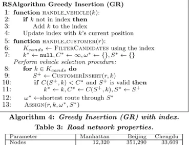
RSAlgorithm Greedy Insertion (GR) 1: functionhandle vehicle(k):

2: ifknot in indexthen 3: Addkto the index

4: Update index withk’s current position 5: functionhandle customer(r):

6: Kcands←FilterCandidatesusing the index 7: k∗_←_{null, C}∗_{← ∞, ω}∗_{← {}, S}∗_{← {}}

Perform vehicle selection procedure: 8: fork∈Kcandsdo

9: S+_←

CustomerInsert(r, k)

10: if C(S+_{, k}₎_{< C}∗_and_S+_{is valid}_then 11: k∗←k, C∗←C(S+_{, k}₎_{, S}∗_←_S+ 12: ω∗←shortest route throughS∗

13: Assign(r, k, ω∗, S∗)

Algorithm 4: Greedy Insertion (GR) with index.

Table 3: Road network properties.

Parameter Manhattan Beijing Chengdu Nodes 12,320 351,290 33,609 Edges 31,444 743,822 73,854

Area (km2) 59 876 643

Total edge length (km) 1,800 17,158 5,117 Road density 30.51 19.59 7.96 Classification dense semi-dense sparse

RSAlgorithm. The RSAlgorithm component represents a

base ridesharing algorithm. The included functions for users to implement their own algorithms are sufficient for a wide range of ridesharing algorithms. The main functions are:

• listen()— Polls for active vehicles and waiting cus-tomers at a configurable interval, storing them locally.

• handle customer(customer)— Executed

automat-ically on every customer that is polled vialisten().

• handle vehicle(vehicle)— Executed automatically

on every vehicle that is polled vialisten().

• match() — Executed at the end of every listen()

and can be used for join-based assignment.

Algorithm 4 shows an example of the greedy algorithm in [27] using RSAlgorithm. This algorithm demonstrates using a specialized index to perform candidates filtering.

Assign Mode. An assign function updates and

synchro-nizes the database with new assignments, routes, and sched-ules. Synchronization is needed due to match latency that equals the time between when a vehicle’s state is first cap-tured to perform assignment and when the assignment is returned to the vehicle. A new assignment could be inval-idated by vehicle motion during this time. For example, an assignment might instruct a vehicle to visit a node it has already passed. Cargo supports two modes. In strict mode, an assignment is rejected outright if it cannot be syn-chronized with the vehicle’s current state. But innon-strict mode, it is accepted if the vehicle can be re-routed to acco-modate the assignment. In preliminary tests, we found that the extra distance due to re-routing is more than offset by extra matches (avoiding the unmatched customers penalty). Hence we use non-strict mode in all our experiments. Spatial Indexes. A G-tree [42] is provided for shortest-path computations, pre-built for each road network in our benchmark and loaded during initiation. A grid index is also provided for quickly filtering vehicles by Euclidean distance as explained in Section 3.2. Users can optionally bring their own spatial index, such as the ones in [27] and [37].

5. BENCHMARK

5.1 Road Networks

We used Manhattan, Beijing, and Chengdu as represen-tative road networks in our benchmarks, listed in Table 3.

(8)

Their different sizes and densities (computed as total edge length divided by area) affect the performance of shortest-path algorithms that ridesharing algorithms rely on. Long edges have been split so that no edge is longer than 100 meters. Each network is a directed graph.

5.2 Problem Instances

Our problem instances aimed to reflect real-world scenar-ios as to give practical insight into algorithm performance. Toward this aim, the number of vehicles, scale of customes, their spatial distributions, and rate of customer requests were most important. We obtained datasets of physical taxi and DiDi trips and used them to generate the customers and vehicles so that spatial distributions and request rates are real. Then when customers were assigned to vehicles dur-ing evaluation, real-time locations of vehicles were simulated based on routes and speeds. Our instances are public [1].

Customers. For each road network, we extracted all taxi

trips occurring in the sampling period from 6:00–6:30PM on an arbitrary day on that network. For Beijing instances, we obtained 17,467 trips, about 9.70 requests per second. For Chengdu and Manhattan instances, we obtained 8,922 and 5,033 trips, respectively, or about 4.96 and 2.80 requests per second. The requests rate can vary at other times, for ex-ample early morning hours or around sporting events. To model these changes, we removed or packed more real trips into the 30-minute period to simulate customer scales of 0.5x, 2.0x, and 4.0x for the Beijing instances. Thesescale factors multiplied the trip sampling period. For each new period, all customers in that period were packed into 30 min-utes, yielding rates of roughly half, double, and quadruple the real requests rate. A small instance where we manually selected 8 customers and 2 vehicles is included to support finding the offline optimal.

Vehicles. All instances use “taxi” vehicles due to better performance as explained in Section 2.2. Initial vehicle po-sitions were sampled from the trip datasets starting from 6:00PM and moving backwards in time until the desired number of vehicles was reached. Each sampled trip origin was used as the initial position of one vehicle. We varied the number of vehicles from 1,000–50,000 to cover real-world scale and beyond. Some studies place the real-world number of ridesharing vehicles to be 13,000 in certain cities [13]. In comparison, most studies use between 100–10,000 vehicles. Capacity varies from 1–9 to cover small passenger vehicles to minibuses. Note that Cargo allows even a 1-capacity taxi to serve an arbitrary number of customers (have long sched-ules) by alternating pickups and dropoffs.

Time Windows. For each customer r, its early bound

was its trip request time in the raw data, relative to 6PM, and its late bound was the shortest-path time between ro and rd, using vehicle speed, plus a delay of 6, 12, or 24 minutes. Taxis in the real world work the entire day instead of appearing throughout the day, thus all taxis had 0 as their early bounds so they appear at the beginning of simulation.

6. EXPERIMENTS

We evaluated the algorithms in Section 3 using Cargo and our benchmarks. We added BA+, a variation of BA with two additional quality heuristics: (1) it only tries replace-ment if the replacing customer has a longer trip than the customer being replaced; and (2) it only accepts a replace-ment if the new route cost is less than before. For SA, we used SA100 and SA50 with hill-climbing factors off= 1.0

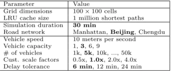
Table 4: Parameters and variables (defaults in bold).

Parameter Value Grid dimensions 100×100 cells LRU cache size 1 million shortest paths Simulation duration 30 min

Road network Manhattan,Beijing, Chengdu Vehicle speed 10 meters per second

Vehicle capacity 1,3, 6, 9

# of vehicles 1k,5k, 10k, ..., 50k Cust. scale factors 0.5x,1.0x, 2.0x, 4.0x Delay tolerance 6 min, 12 min, 24 min

andf= 0.5, respectively, to test usefulness of hill-climbing. For GRASP, we used GP4 and GP16 with 4 and 16 initial solutions, respectively. Offline BB was used to get the opti-mal solution to the sopti-mall instance. Table 4 summarizes our experimental parameters.

Implementation Details.

• Vehicle speed was 10 meters per second (36 kph). • A 100×100 grid index was used to filter vehicles, as

ex-plained in Section 4. Each cell was roughly 300 sq. meters. • For shortest-paths, we used a G-tree with fanout 4. • A least-recently used (LRU) cache with 1 million elements

was used to avoid repeated shortest-path calculations, as in [20]. All algorithms benefited from the cache.

• To mimic a real service guarantee, amatching periodwas used. Customers not matched within 60 seconds of their early bound were not tried again.

• Vehicles with schedules that were larger than 10 elements were pruned for all algorithms. Much time was being spent on these large-schedule vehicles. By doing this prun-ing, the speed of all algorithms improved dramatically. • All algorithms except KT and TG used simple insertion;

KT used kinetic trees while TG used exhaustive insertion for arranging trips in a group.

• For SA100 and SA50 we used T = {5,4...1} and P = 15,000, found to be a good balance of quality and speed. • For TG, the GNU Linear Programming Kit (GLPK)1was used. We allowed top 30 customers per vehicle in step (1) and parallelized all steps as done in [6].

Runtime. Two runtime modes were used. In dynamic

mode, simulation is real-time (one simulated second equals one real second). Instatic mode, Cargo waits until an algo-rithm completes before stepping to the next time instance. To be consistent, all algorithms executed with the same 30-second batch time. Specifically, search algorithms were not executed continuously, but waited until the batch time. Then, they executed sequentially on the batched customers.

Timeouts. A 30-second timeout was necessary for most

algorithms to achieve real-time in dynamic mode. It was applied per customer for search algorithms and per batch for join algorithms. For TG, step (1) was given 15 seconds and the remaining time was allocated to the remaining steps.

Setting. All algorithms were implemented in C++11 and

compiled with the -O3 flag. Experiments were performed on a 2.2 GHz 64-bit Intel Xeon E5-2630 CPU server ma-chine running the Ubuntu 16.04 operating system. Most algorithms used between 1–14 GB RAM depending on the benchmark. Six threads were used for TG.

Metrics. We measured three metrics:

• Average customer handling time, in real milliseconds. • Service rate, the ratio of served customers to total

cus-tomers (a rate of 1 indicates all cuscus-tomers were served). 1

(9)

0 0.2 0.4 0.6 0.8 1.0 1 20 40

Number of Vehicles (thousands) (a) (Search; capacity=1,3,6)

Service Rate

cap.=1

NN GR KT BA BA+

1 20 40

cap.=6

1 20 40

cap.=3 (default) -20 -10 0 10 20 30 40 1 20 40

Number of Vehicles (thousands) (b) (Search; capacity=1,3,6)

Distance Savings (%)

cap.=1

NN GR KT BA BA+

1 20 40 Number of Vehicles (thousands)

(b) (Search; capacity=1,3,6) cap.=6

1 20 40 Number of Vehicles (thousands)

(b) (Search; capacity=1,3,6) cap.=3 (default) 100 101 102 103 1 20 40

Number of Vehicles (thousands) (c) (Search; capacity=1,3,6)

Cust. Handling Time (ms)

cap.=1

NN GR KT BA BA+

1 20 40

cap.=6

1 20 40

cap.=3 (default)

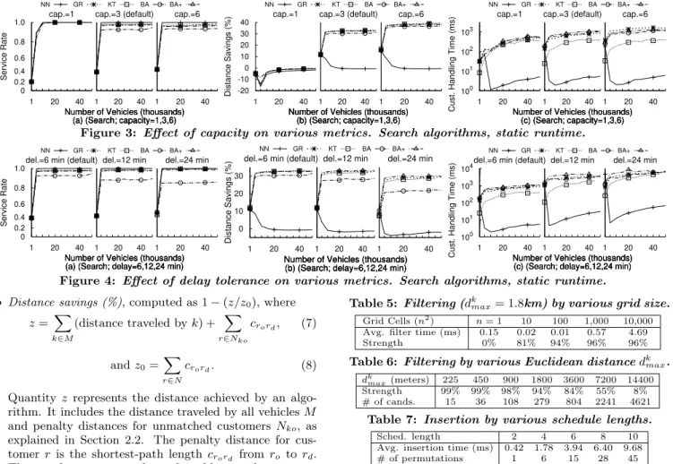
Figure 3: Effect of capacity on various metrics. Search algorithms, static runtime.

0 0.2 0.4 0.6 0.8 1.0 1 20 40

Number of Vehicles (thousands) (a) (Search; delay=6,12,24 min)

Service Rate

del.=6 min (default)

NN GR KT BA BA+

1 20 40

del.=12 min

1 20 40

del.=24 min 0 10 20 30 1 20 40

Number of Vehicles (thousands) (b) (Search; delay=6,12,24 min)

NN GR KT BA BA+

1 20 40

del.=12 min

1 20 40

del.=24 min 100 101 102 103 104 1 20 40

Number of Vehicles (thousands) (c) (Search; delay=6,12,24 min)

NN GR KT BA BA+

1 20 40

del.=12 min

1 20 40

del.=24 min

Figure 4: Effect of delay tolerance on various metrics. Search algorithms, static runtime.

• Distance savings (%), computed as 1−(z/z0), where

z= X k∈M (distance traveled byk) + X r∈Nko crord, (7) andz0= X r∈N crord. (8)

Quantity z represents the distance achieved by an algo-rithm. It includes the distance traveled by all vehiclesM and penalty distances for unmatched customers Nko, as explained in Section 2.2. The penalty distance for cus-tomer r is the shortest-path lengthcrord fromro to rd.

The penalty represents the real-world case where an un-matched customer might elect to take a private vehicle instead of ridesharing. Quantityz0is the sum of all penal-ties, representing the cost of no ridesharing. We call it the

base cost. With ridesharing,zcan be less thanz0because similar trips can be combined (see Example 2). Ifz > z0, then savings is negative, indicating surplus distance.

6.1 Static Runtime Evaluations

We first evaluated candidates filtering and customer in-sertion. Then static mode was used to evaluate the best performance of the algorithms. We varied the number of vehicles because it determines size of Kcands that can af-fect performance of all algorithms. We also varied vehicle capacity to evaluate different capacities used by practition-ers. We omit figures for 9-capacity as no major differences were observed compared to 6-capacity. For join algorithms we varied the customer scale factor because it changes the number of customers per batch and can affect performance.

6.1.1 Filtering and Insertion

As Table 5 shows, our chosen grid size of 100×100 cells achieves the best time at good strength. Strength is com-puted here as 1−(m/M) wheremis the number of candi-dates returned by the filter, andM is the total number of vehicles. Table 5 shows the number of candidates returned by the filter was roughly linear with the filter distancedk

max. Table 6 shows that customer insertion was generally an order of magnitude slower than filtering. The time grew quadrat-ically with schedule length because permutations increased, and to perform insertion, each permutation requires multi-ple shortest-path computations.

Table 5: Filtering (dk

max= 1.8km) by various grid size. Grid Cells (n2₎ _n_{= 1} ₁₀ ₁₀₀ _1,000 _10,000

Avg. filter time (ms) 0.15 0.02 0.01 0.57 4.69 Strength 0% 81% 94% 96% 96%

Table 6: Filtering by various Euclidean distancedkmax.

dk_max(meters) 225 450 900 1800 3600 7200 14400 Strength 99% 99% 98% 94% 84% 55% 8% # of cands. 15 36 108 279 804 2241 4621

Table 7: Insertion by various schedule lengths.

Sched. length 2 4 6 8 10 Avg. insertion time (ms) 0.42 1.78 3.94 6.40 9.68 # of permutations 1 6 15 28 45

6.1.2 Evaluation of Search Algorithms

Effect of Number of Vehicles. More vehicles caused

handling times to increase at all capacities, but had no effect on service rate or distance savings beyond 5,000 vehicles because search algorithms could already match all of the customers at this level (Figure 3). Handling time increased due to more vehicles inKcands to evaluate.

Effect of Vehicle Capacity. At 3-capacity, all except

NN could achieve at least 30% distance savings (roughly 27,000 km) (Figure 3b). The savings are indistinguishable due to all algorithms using the same greedy cost heuristic. Handling time was about one magnitude higher compared to 1-capacity, with a smaller effect for KT, while NN was unchanged (Figure 3c). At 3-capacity, schedules became longer, making customer insertion harder. But NN does not rely on customer insertion and KT uses an index to perform insertion. Notably, NN was faster than all algorithms by two orders of magnitude. Service rate was generally unaffected as 1-capacity was enough to achieve high rates.

Effect of Time Window. Wider time windows had a

small effect on service rate and distance except for BA (Fig-ure 4). With wider windows, BA accepted more replace-ments but could not reassign the displaced customers. As more schedules became feasible, schedules that allowed more travel were accepted and distance savings worsened. On the other hand, BA+ did not experience these effects due to the additional heuristics. Handling time generally increased as there were more valid candidates to evaluate.

(10)

0 0.2 0.4 0.6 0.8 1.0 1 20 40

Number of Vehicles (thousands) (a) (Join; capacity=1,3,6)

Service Rate

cap.=1

SA100 SA50 GP16 GP4 TG

1 20 40

cap.=6

1 20 40

cap.=3 (default) -30 -20 -10 0 10 20 1 20 40

Number of Vehicles (thousands) (b) (Join; capacity=1,3,6)

cap.=1

1 20 40

Number of Vehicles (thousands) (b) (Join; capacity=1,3,6)

cap.=6

1 20 40

Number of Vehicles (thousands) (b) (Join; capacity=1,3,6) cap.=3 (default) 101 102 103 1 20 40

Number of Vehicles (thousands) (c) (Join; capacity=1,3,6)

cap.=1

1 20 40

cap.=6

1 20 40

cap.=3 (default)

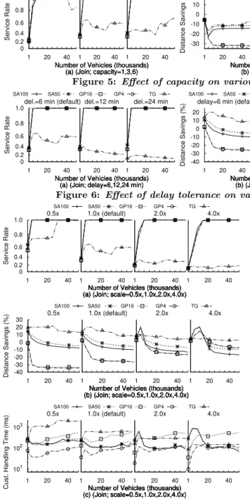
Figure 5: Effect of capacity on various metrics. Join algorithms, static runtime.

0 0.2 0.4 0.6 0.8 1.0 1 20 40

Number of Vehicles (thousands) (a) (Join; delay=6,12,24 min)

Service Rate

1 20 40

del.=12 min

1 20 40

del.=24 min -40 -30 -20 -10 0 10 20 1 20 40

Number of Vehicles (thousands) (b) (Join; delay=6,12,24 min)

delay=6 min (default)

1 20 40

del.=12 min

1 20 40

del.=24 min

102 103 104

1 20 40

Number of Vehicles (thousands) (c) (Join; delay=6,12,24 min)

1 20 40

delay=12 min

1 20 40

delay=24 min

Figure 6: Effect of delay tolerance on various metrics. Join algorithms, static runtime.

0 0.2 0.4 0.6 0.8 1.0 1 20 40

Number of Vehicles (thousands) (a) (Join; scale=0.5x,1.0x,2.0x,4.0x)

Service Rate

0.5x

1 20 40

1.0x (default)

1 20 40

2.0x

1 20 40

4.0x -40 -30 -20 -10 0 10 20 30 1 20 40

Number of Vehicles (thousands) (b) (Join; scale=0.5x,1.0x,2.0x,4.0x)

0.5x

1 20 40

1.0x (default)

1 20 40

2.0x

1 20 40

Number of Vehicles (thousands) (b) (Join; scale=0.5x,1.0x,2.0x,4.0x) 4.0x 101 102 103 1 20 40

Number of Vehicles (thousands) (c) (Join; scale=0.5x,1.0x,2.0x,4.0x)

0.5x

1 20 40

1.0x (default)

1 20 40

2.0x

1 20 40

4.0x

Figure 7: Effect of scale on various metrics. Join

algorithms, static runtime.

Takeaways. Excluding NN, (1)all search algorithms could achieve 100% service rate and more than 30% distance sav-ings; (2) but KT stands out due to best handling time; (3) and simple insertion is acceptable as neither BA, BA+, nor KT could improve distance savings. This result agrees with [27] that the benefit from schedule reordering is small. We did not find BA beating GR in terms of quality as in [14], possibly because the greedy algorithms differed and they used utility score while we used travel distance.

6.1.3 Evaluation of Join Algorithms

On most instances, TG took over 10 hours to run, hence a TG-specific timeout of 10 minutes per batch was added to keep times reasonable. For customer scale experiments, the

requests rate ranged from 4.86 to 36.39 customers per second and the absolute number from 8,754 to 65,500 customers.

Effect of Number of Vehicles. Like search algorithms,

number of vehicles had slight effect beyond 5,000 except to cause handling times to increase (Figures 5c and 6c) because all algorithms already matched near 100% at this level (Fig-ure 5a). In all cases, SA50 used less distance than SA100 because hill-climbing knocked SA100 out of good solutions. The effect may diminish at higherPas there would be more improvement opportunities, but the handling time would in-crease. Also, GP4 achieved the same distances as GP16 but at half the handling time. This result suggests the improve-ment procedures were ineffective, as also observed in [34]. Replacement was not performed because with many vehi-cles, a customer was difficult to be unassigned after initial-ization, and swap rarely selected a valid vehicle due to many candidates in a solution where only a portion are valid for a given customer. Handling time increased for GPs and TG due to largerKcands, but not for SAs as they use random-selectionand do not evaluate all candidates. Different scales altered the effects (Figures 7a, 7b, and 7c).

Effect of Customer Scale. Scale degraded TG and had a

nonlinear effect on GP and SA algorithms. Distance savings by TG decreased as scale increased (Figure 7b) because it ran against the timeout. Handling times for TG actually decreased at larger scales as it had to process more cus-tomers within the same time allotted by the timeout. For GP and SA algorithms, larger scales caused the point at which all customers could be matched to shift. For exam-ple, at 2.0x this point was at 10,000 vehicles but at 4.0x it shifted to 15,000 vehicles (Figure 7a). These algorithms only saved distance before this shifting “saturation” point, and handling times also peaked near the point (Figure 7c). We try to explain these observations about the saturation point. First, regarding service rate, the number of matches for SA and GP algorithms depend on the number of vehi-cles. For both algorithms, the number of matches is prede-termined during the initialization phases as no assignments are added in the improvement phases. If the number of vehi-cles is too few, SA and GP algorithms may not fully initial-ize the customers. The SAs loop through the customers and look for a random feasible vehicle to be a match. Without

(11)

enough vehicles, some customers may not have any feasible candidates and be unmatched. The GPs loop through the vehicles and look for customers to add to each vehicle. The number of matches is thus related to the number of vehi-cles. At some m, all the customers can be initialized and the service rate becomes 1.

Second, two competing factors appear to affect the dis-tance savings. Consider the case where customers are ran-domly distributed amongst m vehicles. If m is very large, then the chance that two customers share one vehicle falls. But ifmis small, then not all customers may be served and the unmatched penalty will be large. At somem, sharing is maximized while the penalty is minimized and savings are greatest. As both SA and GP depend on random selection, this effect appears to a degree.

Third, we found that handling time worsened at the satu-ration point due to longer schedules from many shared trips, making customer insertion harder.

Effect of Vehicle Capacity. Capacity did not affect ser-vice rate or handling time except for TG. Only TG took ad-vantage of 3-capacity to save distance over 1-capacity ure 7b), but with time increases of about one order (Fig-ure 7c). No other algorithms took advantage of capacity.

At 3-capacity, TG made 60% service rate but still achieved 20% distance savings compared to 30% for search algorithms. Figure 7c shows the handling time was flat from hitting the timeout. Thus given better hardware or more processing time, TG may do better than search algorithms.

Effect of Time Window. As with search algorithms,

large time windows increased handling times of all algo-rithms while worsening distance savings (Figure 6). As the number of feasible candidates increases, SAs should require more iterations to converge to a good solution, and the im-provement procedures for GPs were still ineffective due to the previously explained effects.

Takeaways. If hardware is powerful, (1) TG is

recom-mended because it can reliably save travel distancewhile SA and GP algorithms are sensitive to the saturation point. Otherwise, (2) SA50 is preferable over SA100 because it makes slightly better solutions due to less hill-climbing, and (3) GP4 is preferred over GP16 due to faster handling time. We could not confirm that SA uses less distance (time) than GR as in [22], possibly because that study used only 600 ve-hicles and maximum 1.25 customers per second, making it easier for SA to converge to a good solution.

6.2 Real-time Dynamic Evaluations

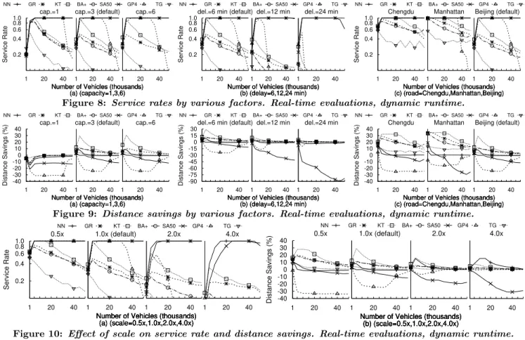
Dynamic runtime mode was used to characterize the real-world performance of the algorithms. We varied number of vehicles, capacity, and customer scale, all factors in the real world. We additionally evaluated performance on Manhat-tan and Chengdu road networks. We omitted BA, SA100 and GP16 based on previous results. We also omitted han-dling times due to the presence of the dynamic runtime time-outs. We show that algorithms mostly could not achieve near their static mode performance.

Effect of Number of Vehicles. For NN, service rate

re-mained high at all numbers of vehicles but no distance sav-ings could be achieved. For the other search algorithms, service rate and distance savings both fell with increasing vehicles. The decline was faster for GR and BA+ com-pared to KT and accelerated at larger scales (Figures 10a and 10b). From the static evaluations, handling time can

increase with more vehicles because Kcands increases. All search algorithms (except NN) perform customer insertion oneach of the candidates, hence take longer when there are more. But in dynamic mode,a long handling time causes the matching rate to fall behind the requests rate. As a result, the queue of customers waiting to be processed fills. After the 60-second matching period expires, customers drop, causing service rate to suffer. Hence thematching rate should meet or exceed the requests rate to ensure good service.

To elaborate, Figure 11 shows the queue size over time on an instance using default parameters. The sawtooth pattern for NN, GP4, and SA50 indicate they could match all cus-tomers within each 30-second batch, explaining their ability for high service rates. Out of the Pgreedy algorithms, KT had the best queue behavior, explaining its ability to save up to 30% travel distance (Figure 9a). For SA50 and GP4, queue size oscillated between 300 and 600 customers because the algorithms took fully 30 seconds allowed by the timeout before returning results, in addition to the 30-second batch time. The lag caused 60 seconds worth of customers to be in the queue. For TG, the queue was nearly always full for all instances, thus it could not achieve a good service rate nor good distance savings.

Effects from the saturation point for SA50 and GP4 dis-appeared because the timeouts limited the processing time. Instead, GP4 experienced a “critical point” where service level dropped dramatically. For example, this point was 30,000 vehicles at 3-capacity (Figure 8a). After this point, GP4 could not initialize full solutions within the timeout due to the expensive repeated fitness evaluations, hence it returned only partial solutions.

Effect of Customer Scale. Algorithms could not meet the

higher request rates at larger scales. Only NN and SA could maintain good service rates (Figure 10a). As scale increased, the critical point for GP4 shifted to lower numbers. For example, at 0.5x the critical point is beyond 50,000 vehicles, but at 2.0x it is 5,000 vehicles.

Effect of Vehicle Capacity. Capacity had little effect

beyond 3 under dynamic runtime as under static runtime.

Effect of Time Window. Service rates for all algorithms

except NN and SA50 dropped with wider time windows (Fig-ure 8b). Distance savings dropped dramatically for SA50 (Figure 9b). With wider time windows, more vehicles be-come feasible, and the chance of randomly selecting the best vehicle per customer becomes smaller. As SA50 depends on random selection to form the initial solution, the chance of forming a good initial solution drops. As it has no time to perform many perturbations in dynamic made, it cannot improve these initial assignments and distance suffers.

Performance on Road Networks. All algorithms could

make more matches and save more distance on Manhattan than on the other two networks (Figures 8c and 9c), and Beijing was the hardest. Customer scale appears to have a stronger effect than road network density. Algorithms achieved highest service rate and most distances savings on dense Manhattan, but performed only slightly worse on sparse Chengdu. Algorithms struggled the most on Beijing, but when scale was reduced to 0.5x, then algorithms could achieve better much service rates (Figure 10a).

Takeaways. Competitive analysis [35] is often used to char-acterize online algorithms. In lieu of theoretical competitive ratios, we ran the algorithms on a small instance against op-timal BB. Table 8 shows the results (obtained after several