Parallel Computing with Mathematica UVACSE Short Course

(1)

Parallel Computing with Mathematica

UVACSE Short Course

E Hall1

1_{University of Virginia Alliance for Computational Science and Engineering}

[email protected]

(2)

Outline

1 NX Client for Remote Linux Desktop

2 Parallel Computing with Mathematica

3 _{Parallel Computing on the Linux Cluster}

4 _References

(3)

Installing and Configuring NX Client

The NX client provides a Gnome Linux desktop interface to the login node of the fir.itc Linux cluster.

http://uvacse.virginia.edu/resources/itc-linux-cluster-overview/the-nx-client/

(4)

Starting and Configuring NX Client

Once logged intofir.itc.virginia.eduthrough NX

Open a terminal from Applications/System Tools/Terminal menu

Select and right-click on Terminal to add to launcher

Create amathematicadirectory withmkdircommand

Start web browser from icon at top of desktop

(5)

Download Short Course Examples

Download the short-course materials from

http://www.uvacse.virginia.edu/software/mathematica-at-uva/

Follow the links,

→Parallel Mathematica

→Parallel Mathematica Short Course

and download 3 files tomathematicadirectory you create with

mkdircommand

ClassExamples_Fa14.zip mathematica-parallel_Fa14.pdf

(6)

Solving Big Technical Problems

Computationally intensive, long-running codes Run tasks in parallel on many processors Task parallel

Large Data sets

Load data across multiple machines that work in parallel Data parallel

(7)

Parallel Computing with Mathematica

Parallel computing in Mathematica is based on launching and

controlling multiple Mathematica kernel (worker) processes from within a single master Mathematica, providing a distributed-memory

environment for parallel programming.

Tested on Unix, Linux, Windows, and Macintosh platforms and are well suited to working locally on a multi-core machine or in a cluster of machines,

(8)

Parallel Computing with Mathematica

To perform computations in parallel, you need to be able to perform the following tasks:

start processes and wait for processes to finish schedule processes on available processors

exchange data between processes and synchronize access to common resources

In the Mathematica environment, the term processor refers to a

running Mathematica kernel, whereas a process is an expression to be evaluated.

(9)

Connection Methods

Mathematica can run parallel workers locally on the same machine or remotely on a compute cluster controlled by a resource management application, e.g. PBSPro.

Local Kernels

The Local Kernels connection method is used to run parallel workers on the same computer as the master Mathematica. It is suitable for a multi-core environment, and is the easiest way to get up and running with parallel computation.

Cluster Integration

The Cluster Integration connection method is used to run parallel workers on a compute cluster from the master Mathematica process. It integrates with the PBSPro cluster management software.

(10)

Parallel Computing Functions

mathematica/guide/ParallelComputing.html

(11)

(12)

Parallel Computing Functions

(13)

Parallel Computing Features

Mathematica supports both task and data parallelism. The main features of parallel computing in Mathematica are:

distributed memory, master/slave parallelism written in Mathematica, machine independent MathLink communication with remote kernels

exchange of symbolic expressions and programs with remote kernels, not only numbers and arrays

virtual process scheduling or explicit process distribution to available processors

virtual shared memory, synchronization, locking

parallel functional programming and automatic parallelization support

(14)

Programming Parallel Applications in Mathematica

To demonstrate demonstrate parallel processing in Mathematica, we useParallelEvaluate. If this is the first parallel computation, it will launch the configured parallel kernels.

(15)

Parallel Kernels Status Monitor

You can open the Parallel Kernels Status monitor through the Evaluation > Parallel Kernel Status menu selection.

(16)

Parallel Preferences

The default settings of Mathematica automatically configure a number of parallel kernels to use for parallel computation, as seen through the Evaluation > Parallel Kernel Configuration menu selection.

(17)

(18)

Launching and Connecting

Mathematica launches parallel kernels automatically as they are needed, but you can also launch kernels manually with the command

LaunchKernels. This is be useful if you were running in a batch mode.

Local Kernels

The Local Kernels connection method supports launching local

kernels directly fromLaunchKernelsby passing it an integer

(setting the number of kernels)

(19)

Launching and Connecting

(20)

Launching and Connecting

Cluster Integration configuration done through Parallel Preferences

(21)

Launching and Connecting

Cluster Integration

The Cluster Integration connection method is used to run parallel workers on the compute nodes of a cluster from the master Mathematica.

The Cluster Integration connection method supports launching

kernels directly fromLaunchKernels. To do so you must first

load the ClusterIntegration‘ package, this is shown below. To launch on a particular cluster you have to pass the name for that cluster into LaunchKernels.

(22)

Launching and Connecting

Cluster Integration

(23)

Sending Commands to Remote Kernels

Values of variables defined on the local master kernel are usually not available to remote kernels.

If you need variable values and definitions carried over to the remote

(24)

Sending Commands to Remote Kernels

Recall that connections to remote kernels, as opened by

LaunchKernels, are represented as kernel objects. The commands below take parallel kernels as arguments and use them to carry out computations.

(25)

Remote Definitions

Mathematica contains a commandDistributeDefinitionsthat

makes it easy to transport local variables and function definitions to all parallel kernels.

Higher-level parallel commands, such asParallelize,

ParallelTable,ParallelSum, ... will automatically distribute definitions of symbols occurring in their arguments.

(26)

Sending Commands to Remote Kernels

(27)

(28)

(29)

(30)

(31)

(32)

Automatically Parallelizing Existing Serial Expressions

Use Parallelize to have Mathematica decide how to distribute work across multiple kernels.

(33)

Automatically Parallelizing Existing Serial Expressions

There is a natural trade-off in parallelization between controlling the overhead of splitting a problem or keeping all the cores busy.

(34)

Sending a Command to Multiple Kernels

UseParallelEvaluateto send commands to multiple kernels and

wait for completion. UseWithto bind locally defined variables before

distribution.

(35)

(36)

Implementing Data-Parallel algorithms

ParallelMapis a natural way to introduce parallelism using a functional programming style. When you have a computationally expensive function to execute of a large data set, Mathematica can execute the operations in parallel by splitting the mapping among multiple kernels.

(37)

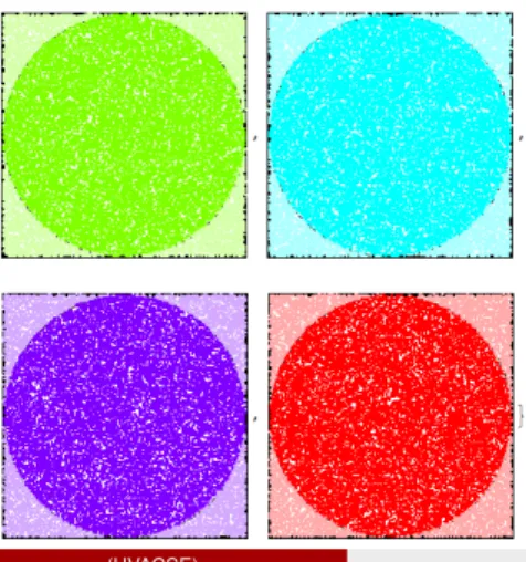
Decomposing a Problem in Parallel Data Sets

(38)

Decomposing a Problem in Parallel Data Sets

Graphic of work distribution among the 4 kernels.

(39)

Decomposing a Problem in Parallel Data Sets

You can generate multiple data sets in parallel, then plot or process them further.

(40)

Choosing an Appropriate Distribution Method

The parallel primitivesParallelize, ParallelMap,

ParallelTable, ParallelDo, ParallelSum,and

ParallelCombinesupport an option calledMethod

It allows you to specify the granularity of the subdivisions used to distribute the computation across kernels.

UseMethod→"FinestGrained"when the completion time of each atomic unit of computation is expected to vary widely.

UseMethod →"CoarseGrained"when the completion time of each atomic unit of computation is expected to be uniform.

(41)

Virtual Shared Memory

Virtual shared memoryis a programming model that allows processors on a distributed-memory machine to be programmed as if they had shared memory. A software layer takes care of the necessary communication in a transparent way.

Mathematica provides functions that implement virtual shared memory for these remote kernels.

The drawback of a shared variable is that every access for read or write requires communication over the network, so it is slower than access to a local unshared variable.

(42)

Mathematica Parallel Workflow

The toolbox enables application prototyping on the desktop with up to 16 local workers (left), and with the Mathematica Cluster Integration package(right), applications can be scaled to multiple computers on a cluster (subsitute Mathematica for Matlab in figure below).

(43)

Scaling Up from the Desktop

Mathematica’s parallel computing provides the ability to use up to 16 local kernels on a multicore or multiprocessor computer.

When used together with Cluster Integration package, you can scale up your application to use any number of kernels running on any number of computers.

ITS Linux cluster allows for 128 kernels.

Alternatively, you can run up to 16 kernels on a single multi-core compute node of the cluster.

(44)

Running Mathematica on Cluster Front-end Node

Mathematica Parallel Computing jobs can be submitted to the ITC Linux cluster by first logging onto the cluster front-end node fir.itc.virginia.edu using the NX client.

Start up Mathematica from a Linux desktop terminal window.

Parallel Mathematica jobs can be submitted from with the Mathematica notebook interface as well as using PBS command files and the

example scripts show how to setup and submit the jobs

Documentation: Submitting Mathematica Parallel Jobs

(45)

(46)

References

1 _{Parallel Computing Tools User Guide}

reference.wolfram.com/mathematica/ParallelTools/tutorial/Overview.html

2 _{Parallel Computing: Mathematica Documentation}

reference.wolfram.com/mathematica/guide/ParallelComputing.html 3 _{Mathematica Cookbook}_{, by Sal Mangano, O’Reilly Press.}

Need further help? Email [email protected].