1
Generating Job Schedules for Vessel Operations
in a Container Terminal
Thin-Yin Leong, Hoong Chuin Lau
Singapore Management University, 80 Stamford Road Singapore (178902), {tyleong, hclau}@smu.edu.sg
Vessel discharge and load jobs in a container terminal can be divided into sequences, one for each assigned quay crane (QC). A QC sequence lists containers in their desired handling order. The common practice for operators is to make do with just this sequence, without generating a job schedule (i.e. desired start-times of handling each container). Operators who need job schedules generate crude ones by using an average gross crane rate (GCR) gleaned from past experience. For realism, the job schedules should recognize the limit the maximum number of prime-movers and yard cranes that it can deploy. In this paper, we study how job schedules can be efficiently generated that maximizes the GCR (or equivalently minimizes the QC total make-span). With an effective algorithm, resources available to a QC can be adjusted, sharing with other QCs, to ensure that its job sequence can be completed by the target end-time. This would lead to more efficient use of terminal resources and good control on the overall vessel completion time.
Keywords: Container terminal, transport scheduling, flowshop, heuristics, quay crane.
1. Introduction
Top ten ports of the world (such as Singapore) have multiple container terminals that are being operated today by competitive corporations, rather than run as a department of their local government. As such, they are increasingly more concerned about competitiveness, cost and service performance than ever before. They now serve concurrently many vessels alongside and their operation hours are being extended to be non-stop round-the-clock. Together with their growth in size to keep up with global demand, they have become more complex to operate.
To better understand the complexity of operations in the terminals, we will describe a typical vessel operation in its fine detail: A vessel discharge job takes 1.5 mins quay crane (QC) cycle to fetch a
container from the vessel. A prime-mover (PM) marries up with the QC and the container is loaded onto the PM's trailer. The PM travels for 8 mins transporting the container from the QC to a yard crane (YC). The YC takes the container off the trailer releasing the PM for its next job, and the YC completes its 3.0 mins cycle time to place the container in a yard location. It then moves to a point ready to serve another PM. A vessel load job would be similarly constructed with the PM arriving at a
YC first and then transporting the container to a QC.
The container discharge and load jobs can be divided into QC sequences, one for each QC assigned to it. A QC sequence lists containers by the container IDs in their desired handling order. Associated with each QC sequence should be a start-time and a target gross crane rate (GCR), i.e. the average number of containers moved in an hour. From these, the target end-time can be deduced.
In this paper, we investigate a real-world problem faced by a container terminal of how job schedules (i.e. desired start-times of handling each container) can be efficiently generated from these sequences. The objective in generating the job schedules is to maximize the GCR or equivalently minimize the QC operation’s total make-span. The typical approach currently practised, without generating a schedule, is to make do with just the QC sequence, because generating a feasible schedule proved to be extremely challenging. Another approach is to generate schedules by using an average GCR gleaned from past experience, without considerations of PM and YC equipment constraints. For realism, the job schedules should recognize the limit the maximum number of PMs and YCs that it
can deploy. With an effective algorithm, resources available to a QC can be adjusted, sharing with other QCs, to ensure that its job sequence can be completed by the target end-time. This would thus lead to more efficient use of terminal resources and good control on the overall vessel completion time. Our problem is very much related to the classical flow-shop scheduling problem. It is in effect a bi-directional flow shop where a job is defined as moving a container from the vessel to a pre-designated yard, or vice versa. Each job comprises 3 tasks – the processing on a QC, the movement by a PM, and the processing by a YC. We are interested in a special constraint that a string of jobs which must be either started or completed in a strict handling sequence for one type of machines (i.e. the QCs). This
constraint is imposed by the need to discharge or load containers in a certain order from the vessel.
2. Literature
Murty et al (2004 and 2005) and Steenken et al (2004) provide excellent descriptions of container terminal operations. Earlier, operations research studies on container terminal operations have focused on high level strategic design and tactical planning problems: demand forecasting, terminal and berth capacity planning, berth planning, vessel stowage planning and yard planning. There have not been as many studies on operational scheduling and control concerns as these problems tend to be complex, and unless properly handled is best left to practitioners to work out in real-time operational execution. Otherwise, constraint programming and artificial intelligence methods are used. Artificial Intelligence (AI) methods are extremely difficult to implement in real-life and are often avoided by practitioners. So very few are actually implemented into real systems, especially those commercially available.
To support potential automation of the terminals with automated guided vehicles (AGVs) and automatic stacking cranes (ASCs), these complex problems and solution approaches can no longer be avoided. Liu et al (2002) and Bish et al (2001 and 2005) consider the scheduling and dispatching of PMs to support QC operations, addressing specific problems like vehicle routing, job dispatching etc. which container terminal operators cannot force compliance on the PM drivers, and may be they can do a better job finding the best route. Steenken et al 2000 considers the need to coordinate transport and stowage in shipping planning.
Recently, there is a surge of studies (e.g. Zhu and Lim 2004, Ng and Mak 2006, Jung and Kim2006) on discovering the optimal “crane split” of vessel discharge and load jobs among the QCs for a single vessel. This problem is similar to the production line balancing problem. The output of this would be a sequence for each QC, but these studies largely assume infinite terminal resources to support the
QCs. Such problems for the whole container terminal (Moccia et al 2005) are complex and large
mixed integer programs, requiring branch-and-cut, agent-based AI and heuristics approaches.
3. Problem Formulation
We now state the notations (refer to Figure 1) for describing the mathematical formulation of our problem. Consider a QC sequence. For the thcontainer in this sequence,
i i=1,...,n, let be the job
type, be the job start-time and be the job end-time on equipment
i T ji S Eji j, where denotes QC,
{
u,x,y}
j∈u xdenotes PM and denotes YC.
y
Ti∈{
Disc,Load}
, where denotes dischargeand denotes load jobs. C and respectively are the QC and YC cycle times (which can
be simply and if independent of ) and C is the PM travel time, computed by dividing the
approximate distance between the container’s current location to its destination with the average PM
speed. There is also an interface time C , specified as the minimum time required between a PM
Disc Load ui Cyi i u C
C
y xi ffrom its trailer. In general, all time durations . By definition, the relationships between the variables are as follows:
0 .. ≥ C 3
}
{
u y j n i C S Eji ≡ ji + ji, =1,... , ∈ , (1) n i T if C C S C E T if C C S C E S f yi yi j yi f ui ui f ui xi , , 1,... , = ⎩ ⎨ ⎧ − + = − − + = − ≡ Load Disc i i = = n ,... 1 (2) i Load T if C S Disc T if C S E i j ui i f yi xi , , , = ⎩ ⎨ ⎧ = + = + ≡ (3) Vessel Discharge Vessel Load Cui Eyi Syi Cf Eui Syi Eyi Sui Eui Sui ≥ Cxi ≥ Cxi Cyi Cui Cyi Cf Cf Cf PM YC QC YC PM QCFigure 1. Vessel Discharge and Vessel Load Jobs Time Elements
The problem is to determine Sui and Syi for i=1,...,n, which in turn defines and all the job end-times since the cranes and PMs must work hand-in-hand transferring the containers between them.
xi
S
The Job Schedule Generation Problem is formulated formally as follows:
(
GenSch
XY)
:MinimizeZ =Eun [or Maximize GCR=n/(Eun −Su1)] (4)
subject to n i E Sui ≥ ui−1, =2,... (5)
{
k S Sxi Exk,k n}
i n D where X D n( xi)≤ xi = : xk ≤ < =1,..., , =1,... (6){
k S S k n}
i n D where Y D n( yi)≤ yi = : yk ≤ yi <Eyk, =1,..., , =1,... (7) n i Load T if C E S Disc T if C E S i xi yi ui i xi ui yi ,... 1 , , , = = ≥ − = ≥ − (8) 0 ≥ ui S and Syi≥
0
for i=
1
,...
,
n. (9)Objective function (4) minimizes the make-span, i.e. the completion time of the QC sequence. is the start-time of the first QC job and also the sequence start-time. Without loss of generality, we let . Constraint (5) specifies that the QC handling order and its capacity are not violated. Constraints (6) and (7) ensure respectively that the number of PMs and YCs deployed at the start-time of any job i do not exceed the available
1 u S
0
1=
u SX
prime movers andY
yard cranes. Since increase inequipment deployed happens only at the start-times of PM and YC jobs, constraints (6) and (7) will
ensure that limitsX and Y are not exceeded for the whole duration of working the QC sequence.
Constraint (8) states that the separation time between crane handlings at both ends of a PM travel must be at least as long as the travel time so that it is physically possible to execute. Constraint (9) is the
non-negativity constraint on the crane start-times. The optimal schedule of will be referred
to as .
XY
GenSch
SchOpt
One decision problem associated with is: Is there a schedule with make-span no greater
than a given value Z using no more than X PMs (or no more than Y YCs, or both)? Note that if there
is no restriction on the QC handling sequence, this problem is NP-complete, since the Bin-Packing
problem can be trivially reduced to it by treating each PM as a bin and Z as the bin capacity.
Interestingly, when the QC sequence is strictly imposed, this problem can be nicely solved by a greedy algorithm, as we will show in the next section.
XY
GenSch
4. Solution Approaches
It can be observed that good schedules for should pack the jobs tightly, with minimal time
gaps between the end of one QC job and the start of the next QC job. Hence, one approach for generating a job schedule is to pack the jobs one after another, so long as they follow the QC handling
sequence constraint. This algorithm (denoted as ) would generate the highest possible GCR, but
violates the PM and YC availability constraints.
XY
GenSch
1
Sch
Load Load T if C C Sui xi yi, i ⎩ − − =n
i
S
ui,
=
2
,
...,
yi,
i=
1
,
...,
n ∞ XGenSch
2
X∞In the case where we do not permit the PM jobs to wait, we can simplify by replacing definitions (2) and (3) with (10) and (11) and adding constraint (12):
n i Disc T if C C S Sxi ≡ ⎨⎧ ui + ui − f, i = , =1,... (10) T if C C Sui xi f, i ⎩ − − = n i C C S Exi ≡ xi + xi +2 f, =1,... n i Disc T if C C S Syi ≡ ⎨⎧ ui+ ui + xi, i = , =1,... (11) (12) Invoking constraints (10) and (11) together is the same as changing the inequality in (8) to equality,
making the constraint binding. This resulting problem will be referred to as , under
which only is a decision variable; formerly a decision variable, S is
now a dependent variable. That is, we need only find the QC job times, as the rest of the start-times can be easily derived by adding or subtracting the cycle, travel and interface start-times.
XY
GenSch
2
(and hence
GenSch
) can be solved optimally using a greedy algorithm, both for agiven set of purely discharge jobs or purely load jobs. In the following, we will present our algorithm for the case of discharge jobs, followed by load jobs. It turns out that the latter algorithm is identical to the former, in reverse time sequence, as we will demonstrate.
Scheduling Discharge Jobs: We assign jobs in increasing QC handling order. For each job i, we
assign its start time to be the earliest time that does not violate the PM and YC capacities. In other words, is the earliest time such that (1) is no earlier than the end time of job i-1; (2) is the
time when a PM is available; and (3) is the time when a YC is available. Let this algorithm be
denoted as Sch-Discharge. ui
S Sui Sxi
yi
S
Scheduling Load Jobs: Again, we assign jobs in increasing QC handling order. The trick here is to
think of load jobs as discharge jobs in a reverse time sequence – so we perform scheduling in a
reverse time sequence where the QC task becomes the first instead of the last task. In doing so, we shift the burden to maintain QC handling order at the end to the beginning, and hence the same
algorithm in Sch-Discharge may be applied. After scheduling, we simply reverse again the start and
end times of each job. This trick has been shown to work for the problem discussed in Bish et al (2005). Let this algorithm be denoted as Sch-Load.
4.1 Analysis
5
∞ X XY ∞ X ∞ X XY 2Both Sch-Discharge and Sch-Load can be implemented to solve in worst-case time
complexity of O(n log X). For each job, it suffices to determine when a PM would be available. If we
maintain a heap of size X which contains the completion timings of each PM, then obtaining the
earliest completion time of a PM and updating the new completion time (as a result of a job assignment) is equivalent to performing a decreaseKey operation on the respective heap, which takes
logarithmic time. This also means that if X is constant, then we have a linear time greedy algorithm
to solve
GenSch
. For the general case , the situation is slightly tricky since there couldbe cases when a PM is available but a YC is not, and vice versa. To ensure that we find the earliest available time slot to assign a job, we need to scan from the earliest available time of a PM forward until the time when a YC is available. Typically, since the YC cycle is short, this scan is negligible
∞ X
GenSch
GenSch
2
In the following, we will prove that both Sch-Discharge and Sch-Load are optimal for restricted cases.
Proposition 1: Sch-Discharge is optimal to
GenSch
2
if all jobs are discharge jobs.Proof:
This can be shown by an exchange
argument as follows. Denote the schedule obtained bySch-Discharge as Sch. Suppose that there exists an optimal schedule SchOpt that is not the same as Sch. Consider each job assignment in SchOpt from 1 to n in that order. Let job i be the first job
whose start time is different from Sch. Let the start times of this job be denoted Sui and SuiOPT
respectively. Since the start-time for job i in Sch is the earliest possible, we have Sui< SuiOPT. Now
shift the start-time of job i in SchOpt backward from SuiOPT to Sui.. Note that this will not introduce
infeasibility with the jobs before i, since Sch is a feasible schedule. Clearly, shifting backwards will
also not affect the feasibility of the jobs after i. Furthermore, the resulting make-span will either
remain or improve. Following this argument inductively, we can convert SchOpt to Sch without
affecting the make-span. Hence, Sch is also an optimal schedule. □
Corollary: Sch-Load is optimal to
GenSch
2
if all jobs are load jobs.Proof: Again, a simple argument as above can show this.
Unfortunately, the above algorithm is not optimal for GenSch in general. Consider the following
counter example comprising a sequence of 6 pure discharge jobs where the QC and YC cycle times are 1 and 2 respectively, PM travel times are 10, 9, 10, 7, 6, 20 respectively, and capacities X=6 and Y=2. In this case, Sch-Discharge produces a make-span of 32 while the optimal make-span is 30.
Thus far, we have considered algorithms for purely discharge or purely load jobs. If we are given a
mixed sequence of discharge followed by load jobs, then it is technically cumbersome to switch
between Sch-Discharge and Sch-Load. Furthermore, this presents the additional challenge to splice
the solutions together in a manner that can exploit savings at the cross-over time region between discharge and load jobs. For instance, some discharge jobs might be deferred to allow some load jobs to start earlier, so that the QC will not need to wait for the load jobs to arrive upon completion of all discharge jobs.
In the following we will consider a new single-pass forward algorithm to handle mixed job sequences. This algorithm is simple, efficient and effective (see Experiments section). Unfortunately, it does not preserve the optimality property presented in Propositions 1 and 2. It will however do so if we
consider a restricted version of the problem. We define function to return the
largest value, and replace constraints (6) and (7) by (13) and (14): XY GenSch2 MAXm th m
(
E k i)
i n MAX Sxi ≥ X xk : =1,..., −1 =2,... (13)(
E k i)
i n MAX Syi ≥ Y yk : =1,..., −1 =2,... (14) XY GenSch2 ⇒ XYGenSch
modified as above will be referred to as . It is clear that (13) (6) and (14)
(7). Hence, feasible solutions to GenSch provide feasible and upper bound solutions
to . XY GenSch3 XY ⇒ 3
The following greedy algorithm is proposed: Start sequentially from job to find
and then compute the rest using (1), (10), (11) and (12). Using the property of constraints (13) and (14), the feasible solution for each job
i
can be found by shifting only jobi
forward so that its PM job start-time is not earlier than the largest end-time from among all the PM jobs preceding it andits YC job’s start-time is not earlier than the largest end-time from among all the YC jobs
preceding it. Again, we seek to restore feasibility with least delay to job
i
. Both algorithms generate the job start-times for QC, PM and YC jobs in a single pass, without violating the handling order ofQC jobs or exceeding and
Y
(the PM and YC availability limits). It can be shown that Sch isoptimal for . XY Sch3 th
X
2
=
i
S
ui XY thY
X
XY 3 GenSch35. Experiments and Discussions
In this section, we report computational experiments to test the efficiency of the algorithms and quality of results measured in real-world terms. Extensive experimental results that compare our heuristics with other heuristics and exact MIP models have been reported in a separate paper (see Zhao et al 2007).
A total of 432 realistic test cases were generated for the foll
owing data values (all times in
minutes): Cf
=
0
.
25
,
Cu∈
{
1
.
0
,
1
.
5
,
2
.
0
}
,
Cy∈
{
2
.
3
,
3
.
0
,
3
.
5
}
,
Cxi∈
{
8
±
4
,
10
±
5
,
12
±
6
}
(uniformly-distributed), X∈
{
4,5,6,7}
and Y∈{
2,3,4,5}
. For each test case, a QC job sequence of 100 jobs is randomly generated, with 50 discharge jobs followed immediately by 50 load jobs. Wecompute the following results: average (approx.) and maximum PMs and YCs used under ,
maximum number YC used and number of times more than
XY
Sch
3
Y
YCs are used under , and GCRunder ,
Sch
andSch
.∞ X
Sch
3
SchOpt
3
XY3
X∞(1) is near-optimal with = -0.3% average and -3.6%
maximum. takes 5sec to 43sec to compute, averaging at 22sec. With ≈
and running in sub-second time, we conclude that in real life, constraints (10)
to (12) are generally reasonable assumptions to make and offers a very practical
near-optimal approach. XY
Sch
3
SchOPTGCR
SchOpt SchOpt SchGCR
GCR
GCR
XY)
/
(
3−
XYSch
3
SchOptSch
XY SchGCR
3 XY3
(2) was found to be better than optimal: = 4.4%
average and 33.5% maximum. It is of course infeasible relative to the constraint on
∞ X
Sch
3
(
GCR
Sch3X∞−
GCR
SchOpt)
/
GCR
SchOptY
YCs. However, the number of timesY
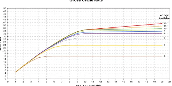
was violated was found to be moderate: 11 jobs on average and 55 jobs maximum out of 100.Using our proposed scheme for generating job schedules , we are able to examine the
relationship between GCR and various PM/QC and YC/QC available ratios, which is shown in Figure 2. The GCR increases with PM/QC rising linearly and then saturates at different levels that increases with YC/QC. This is consistently with what is observed in actual terminal operations, though they usually track the relationship to the deployed ratios rather than the availability limits.
XY
Sch
3
Gross Crane Rate
20 15 10 5 4 3 2 1 0 2 4 6 8 10 12 14 16 18 20 22 24 26 28 30 32 34 36 38 40 42 44 46 48 50 0 1 2 3 4 5 6 7 8 9 10 11 12 13 14 15 16 17 18 19 20 21 PM / QC Available Mo v e / H o u r YC / QC Available
Figure 2: Gross Crane Rate vs PM and YC equipment available
6. Concluding Remarks
The most critical resource in the container terminals is usually not the YC: YC holding is typically almost four times that of QC. The liberal relative quantities of YC is mostly to cater for the fact that YCs are physically distributed over a very large area and they are not mobile enough to be quickly moved from one location to another location. Hence, the key issue is not YC availability but activating the right sub-set of YCs. The terminals can usually do with more PMs since QC is the most expensive resource of the three, and thus should not be slowed down unnecessarily by the lack of YCs or PMs. But having too many PMs without highly sophisticated coordination means would only lead to queues in the wrong places and massive traffic congestion. Hence the controlling variable in container terminal productivity is usually PM availability. For this reason, we can safely focus on
rather than GenSch∞Y.
∞
X
GenSch
We observe that the number of YC deployed does not go frequently above reasonable Y limits when the schedule is generated using Sch3X∞.. In fact, the number YCs used are often below
Y
, i.e.constraint (7) is usually non-binding. This suggests that we may not need to constraint YCs and let it be an outcome of the PM/QC availability instead. Additional YCs required, beyond base availability given, may be marshaled for blocks of time from other QCs. Conversely, this QC can share its YCs with other QCs when they need them for short periods of time. Therefore, the result exploited in a multiple QCs situation would result in higher GCRs for all QCs, with no additional investment in YCs by the container terminal.
Without loss of generality, we have made simplifying assumptions in our study, e.g. each PM carries only one container and only one yard location is visited per PM trip. Further operational refinements are needed for deploying the proposed algorithm in container terminal operations, which include these and many other practical details. These additions however would not compromise or alter the nature of results reported here. As an example, we may replace PMs in our model with straddle carriers (SCs), the alternative mover-stacker used in terminal operations. SC terminal operations has the advantages that no YCs are needed since SCs can stack containers in the yard, and QCs and SCs do not have to wait for each other as they can put and pickup containers from the wharf side, i.e. their operations are de-synchronized within reasonable limits. Our results will still apply.
In this paper, we considered job scheduling for a single QC. In a continuing work, we study a decentralized multi-QC coordination problem where resources (PM, YCs) are shared. There, we employ a combinatorial auction mechanism to broker the utilization of shared resources to conflicting demands arising from multiple QCs. The algorithm proposed in this paper provides the base algorithm for individual QCs (bidders) to generate their optimal resource bundle bids to be submitted to the auctioneer.
References
[1] Bish, Leong, Li, Ng and Simchi-Levi (2001), Analysis of a New Vehicle Scheduling and Location Problem, Naval Research Logistics48(5), 363 – 385.
[2] Bish, Chen, Leong, Nelson, Ng and Simchi-Levi (2005), Dispatching Vehicles in a Mega Container Terminal, OR Spectrum27(4), 491 – 506.
[3] Jung and Kim (2006), Load scheduling for multiple quay cranes in port container terminals,
Journal of Intelligent Manufacturing17(4), 479 – 492.
[4] Liu, Jula and Ioannou (2002), Design, simulation, and evaluation of automated container, IEEE Transactions on Intelligent Transportation Systems3(1), 12 – 26.
[5] Moccia, Cordeau, Gaudioso and Laporte (2005), A branch-and-cut algorithm for the quay crane scheduling problem in a container terminal, Naval Research Logistics53(1), 45 – 59.
[6] Murty, Liu, Wan and Linn (2004), A decision support system for operations in a container terminal, Decision Support Systems39(3), 309 – 332.
[7] Murty, Wan, Liu, Tseng, Leung, Lai and Chiu (2005), Hong kong International Terminals Gains Elastic Capacity Using a Data-Intensive Decision-Support System, Interfaces 35(1), 61 –75.
[8] Ng and Mak (2006), Quay crane scheduling in container terminals, Engg Optimization38(6), 723 –737.
[9] Steenken, Voβ and Stahlbock (2004), Container terminal operations and operations research – a classification and literature review, OR Spectrum26, 3 – 49.
[10] Zhao, Leong, Ge, and Lau (2007), Bidirectional Flow Shop Scheduling with Multi-Machine Capacity and Critical Operation Sequencing, Proc. 22nd IEEE International Symp. on Intelligent Control.
[11] Zhu and Lim (2004), Crane Scheduling with Spatial Constraints: Mathematical Model and Solving Approaches, Proc. 8th International Symp. AI and Math, Florida, USA.