CHAPTER 5
MEASURING RETURN ON INVESTMENTS
In Chapter 4, we developed a process for estimating costs of equity, debt, and capital and presented an argument that the cost of capital is the minimum acceptable hurdle rate when considering new investments. We also argued that an investment has to earn a return greater than this hurdle rate to create value for the owners of a business. In this chapter, we turn to the question of how best to measure the return on a project. In doing so, we will attempt to answer the following questions:
• What is a project? In particular, how general is the definition of an investment and what are the different types of investment decisions that firms have to make?
• In measuring the return on a project, should we look at the cash flows generated by the project or at the accounting earnings?
• If the returns on a project are unevenly spread over time, how do we consider (or should we not consider) differences in returns across time?
We will illustrate the basics of investment analysis using four hypothetical projects: an online book ordering service for Bookscape, a new theme park in Brazil for Disney, a plant to manufacture linerboard for Aracruz Celulose and an acquisition of a US company by Tata Chemicals.
What Is a Project?
Investment analysis concerns which projects a company should accept and which it should reject; accordingly, the question of what makes up a project is central to this and the following chapters. The conventional project
analyzed in capital budgeting has three criteria: (1) a large up-front cost, (2) cash flows for a specific time period, and (3) a salvage value at the end,
which captures the value of the assets of the project when the project ends. Although such projects undoubtedly form a significant proportion of investment decisions, especially for manufacturing firms, it would be a mistake to assume that investment analysis stops there. If a project is defined more broadly to include any decision that results in using the Salvage Value: The estimated liquidation value of the assets invested in the projects at the end of the project life.
scarce resources of a business, then everything from strategic decisions and acquisitions to decisions about which air conditioning system to use in a building would fall within its reach.
Defined broadly then, any of the following decisions would qualify as projects:
1. Major strategic decisions to enter new areas of business (such as Disney’s foray into real estate or Deutsche Bank’s into investment banking) or new markets (such as Disney television’s expansion into Latin America).
2. Acquisitions of other firms are projects as well, notwithstanding attempts to create separate sets of rules for them.
3. Decisions on new ventures within existing businesses or markets, such as the one made by Disney to expand its Orlando theme park to include the Animal Kingdom or the decision to produce a new animated movie.
4. Decisions that may change the way existing ventures and projects are run, such as programming schedules on the Disney channel or changing inventory policy at Bookscape.
5. Decisions on how best to deliver a service that is necessary for the business to run smoothly. A good example would be Deutsche Bank’s choice of what type of financial information system to acquire to allow traders and investment bankers to do their jobs. While the information system itself might not deliver revenues and profits, it is an indispensable component for other
revenue generating projects.
Investment decisions can be categorized on a number of different dimensions. The first relates to how the project affects other projects the firm is considering and analyzing. Some
projects are independent of other projects, and thus can be analyzed separately, whereas other projects are mutually exclusive—that is, taking one project will mean rejecting other projects. At the other extreme, some projects are prerequisites for other projects down the road and others are complementary. In general, projects can be categorized as falling somewhere on the continuum between prerequisites and mutually exclusive, as depicted in Figure 5.1.
Mutually Exclusive Projects: A group of projects is said to be mutually exclusive when acceptance of one of the projects implies that the rest have to be rejected.
Figure 5.1 The Project Continuum
The second dimension that can be used to classify a project is its ability to generate revenues or reduce costs. The decision rules that analyze revenue-generating projects attempt to evaluate whether the earnings or cash flows from the projects justify the investment needed to implement them. When it comes to cost-reduction projects, the decision rules examine whether the reduction in costs justifies the up-front investment needed for the projects.
Illustration 5.1: Project Descriptions.
In this chapter and parts of the next, we will use four hypothetical projects to illustrate the basics of investment analysis.
• The first project we will look at is a proposal by Bookscape to add an online book ordering and information service. Although the impetus for this proposal comes from the success of other online retailers like Amazon.com, Bookscape’s service will be more focused on helping customers research books and find the ones they need rather than on price. Thus, if Bookscape decides to add this service, it will have to hire and train well-qualified individuals to answer customer queries, in addition to investing in the computer equipment and phone lines that the service will require. This project analysis will help illustrate some of the issues that come up when private businesses look at investments and also when businesses take on projects that have risk profiles different from their existing ones.
• The second project we will analyze is a proposed theme park for Disney in Rio De Janeiro, Brazil. Rio Disneyworld, which will be patterned on Disneyland Paris and Walt Disney World in Florida, will require a huge investment in infrastructure and take several years to complete. This project analysis will bring several issues to the forefront, including questions of how to deal with projects when the cash flows are in a foreign currency and what to do when projects have very long lives.
• The third project we will consider is a plant in Brazil to manufacture linerboard for Aracruz Celulose. Linerboard is a stiffened paper product that can be transformed into cardboard boxes. This investment is a more conventional one, with an initial investment, a fixed lifetime, and a salvage value at the end. We will, however, do the analysis for this project from an equity standpoint to illustrate the generality of investment analysis. In addition, in light of concerns about inflation in Brazil, we will do the analysis entirely in real terms.
• The final project that we will examine is Tata Chemical’s proposed acquisition of Sensient Technologies, a publicly traded US firm that manufactures color, flavor and fragrance additives for the food business. We will extend the same principles that we use to value internal investments to analyze how much Tata Chemicals can afford to pay for the US company and the value of any potential synergies in the merger. We should also note that while these projects are hypothetical, they are based upon real projects that these firms have taken in the past.
Hurdle Rates for Firms versus Hurdle Rates for Projects
In the previous chapter we developed a process for estimating the costs of equity and capital for firms. In this chapter, we will extend the discussion to hurdle rates in the context of new or individual investments.
Using the Firm’s Hurdle Rate for Individual Projects
Can we use the costs of equity and capital that we have estimated for the firms for these projects? In some cases we can, but only if all investments made by a firm are similar in terms of their risk exposure. As a firm’s investments become more diverse, the firm will no longer be able to use its cost of equity and capital to evaluate these projects. Projects that are riskier have to be assessed using a higher cost of equity and capital than projects that are safer. In this chapter, we consider how to estimate project costs of equity and capital.
What would happen if a firm chose to use its cost of equity and capital to evaluate all projects? This firm would find itself overinvesting in risky projects and under investing in safe projects. Over time, the firm will become riskier, as its safer businesses find themselves unable to compete with riskier businesses.
Cost of Equity for Projects
In assessing the beta for a project, we will consider three possible scenarios. The first scenario is the one where all the projects considered by a firm are similar in their exposure to risk; this homogeneity makes risk assessment simple. The second scenario is one in which a firm is in multiple businesses with different exposures to risk, but projects within each business have the same risk exposure. The third scenario is the most complicated wherein each project considered by a firm has a different exposure to risk. 1. Single Business; Project Risk Similar within Business
When a firm operates in only one business and all projects within that business share the same risk profile, the firm can use its overall cost of equity as the cost of equity for the project. Because we estimated the cost of equity using a beta for the firm in Chapter 4, this would mean that we would use the same beta to estimate the cost of equity for each project that the firm analyzes. The advantage of this approach is that it does not require risk estimation prior to every project, providing managers with a fixed benchmark for their project investments. The approach is restricting, though, because it can be usefully applied only to companies that are in one line of business and take on homogeneous projects.
2. Multiple Businesses with Different Risk Profiles: Project Risk Similar within Each Business
When firms operate in more than one line of business, the risk profiles are likely to be different across different businesses. If we make the assumption that projects taken within each business have the same risk profile, we can estimate the cost of equity for each business separately and use that cost of equity for all projects within that business. Riskier businesses will have higher costs of equity than safer businesses, and projects taken by riskier businesses will have to cover these higher costs. Imposing the firm’s cost of equity on all projects in all businesses will lead to overinvesting in risky businesses (because the cost of equity will be set too low) and under investing in safe businesses (because the cost of equity will be set too high).
How do we estimate the cost of equity for individual businesses? When the approach requires equity betas, we cannot fall back on the conventional regression
approach (in the CAPM) or factor analysis (in the APM) because these approaches require past prices. Instead, we have to use one of the two approaches that we described in the last section as alternatives to regression betas—bottom-up betas based on other publicly traded firms in the same business, or accounting betas, estimated based on the accounting earnings for the division.
3. Projects with Different Risk Profiles
As a purist, you could argue that each project’s risk profile is, in fact, unique and that it is inappropriate to use either the firm’s cost of equity or divisional costs of equity to assess projects. Although this may be true, we have to consider the trade-off. Given that small differences in the cost of equity should not make a significant difference in our investment decisions, we have to consider whether the added benefits of analyzing each project individually exceed the costs of doing so.
When would it make sense to assess a project’s risk individually? If a project is large in terms of investment needs relative to the firm assessing it and has a very different risk profile from other investments in the firm, it would make sense to assess the cost of equity for the project independently. The only practical way of estimating betas and costs of equity for individual projects is the bottom-up beta approach.
Cost of Debt for Projects
In the previous chapter, we noted that the cost of debt for a firm should reflect its default risk. With individual projects, the assessment of default risk becomes much more difficult, because projects seldom borrow on their own; most firms borrow money for all the projects that they undertake. There are three approaches to estimating the cost of debt for a project:
• One approach is based on the argument that because the borrowing is done by the firm rather than by individual projects, the cost of debt for a project should be the cost of debt for the firm considering the project. This approach makes the most sense when the projects being assessed are small relative to the firm taking them and thus have little or no appreciable effect on the firm’s default risk.
• Look at the project’s capacity to generate cash flows relative to its financing costs and estimate default risk and cost of debt for the project, You can also estimate
this default risk by looking at other firms that take similar projects, and use the typical default risk and cost of debt for these firms. This approach generally makes sense when the project is large in terms of its capital needs relative to the firm and has different cash flow characteristics (both in terms of magnitude and volatility) from other investments taken by the firm and is capable of borrowing funds against its own cash flows.
• The third approach applies when a project actually borrows its own funds, with lenders having no recourse against the parent firm, in case the project defaults. This is unusual, but it can occur when investments have significant tangible assets of their own and the investment is large relative to the firm considering it. In this case, the cost of debt for the project can be assessed using its capacity to generate cash flows relative to its financing obligations. In the last chapter, we used the bond rating of a firm to come up with the cost of debt for the firm. Although projects may not be rated, we can still estimate a rating for a project based on financial ratios, and this can be used to estimate default risk and the cost of debt.
Financing Mix and Cost of Capital for Projects
To get from the costs of debt and equity to the cost of capital, we have to weight each by their relative proportions in financing. Again, the task is much easier at the firm level, where we use the current market values of debt and equity to arrive at these weights. We may borrow money to fund a project, but it is often not clear whether we are using the debt capacity of the project or the firm’s debt capacity. The solution to this problem will again vary depending on the scenario we face.
• When we are estimating the financing weights for small projects that do not affect a firm’s debt capacity, the financing weights should be those of the firm before the project.
• When assessing the financing weights of large projects, with risk profiles different from that of the firm, we have to be more cautious. Using the firm’s financing mix to compute the cost of capital for these projects can be misleading, because the project being analyzed may be riskier than the firm as a whole and thus incapable of carrying the firm’s debt ratio. In this case, we would argue for the
use of the average debt ratio of the other firms in the business in assessing the cost of capital of the project.
• The financing weights for stand-alone projects that are large enough to issue their own debt should be based on the actual amounts borrowed by the projects. For firms with such projects, the financing weights can vary from project to projects, as will the cost of debt.
In summary, the cost of debt and debt ratio for a project will reflect the size of the project relative to the firm, and its risk profile, again relative to the firm. Table 5.1 summarizes our analyses.
Table 5.1 Cost of Debt and Debt Ratio: Project Analyses
Project Characteristics Cost of Debt Debt Ratio
Project is small and has cash flow characteristics similar to the firm
Firm’s cost of debt Firm’s debt ratio
Project is large and has cash flow characteristics
different from the firm
Cost of debt of comparable firms (if non-recourse debt) or the firm (if backed by the firm’s creditworthiness)
Average debt ratio of comparable firms
Stand-alone project Cost of debt for project (based on actual or synthetic ratings)
Debt ratio for project
Illustration 5.2: Estimating Hurdle Rates for Individual Projects
Using the principles of estimation that we just laid out, we can estimate the hurdles rates for the projects that we are analyzing in this chapter.
• Bookscape Online Information and Ordering Service: Because the beta and cost of equity that we estimated for Bookscape as a company reflect its status as a book store, we will re-estimate the beta for this online project by looking at publicly traded Internet retailers. The unlevered total beta of internet retailers is 4.25,1 and we assume that this project will be funded with the same mix of debt and equity (D/E = 53.47%, Debt/Capital = 34.84%) that Bookscape uses in the rest of the business. We will assume that Bookscape’s tax rate (40%) and pretax cost of debt (6%) apply to this project.
1The unlevered market beta for internet retailers is 1.70, and the average correlation of these stocks with the
Levered Beta Online Service = 4.25 [1 + (1 – 0.4) (0.5357)] = 5.61
Cost of Equity Online Service = 3.5% + 5.61 (6%) = 37.18%
Cost of CapitalOnline Service= 37.18% (0.6516) + 6% (1 – 0.4) (0.3484) = 25.48%
This is much higher than the cost of capital we computed for Bookscape in chapter 4, but it reflects the higher risk of the online retail venture.
• Rio Disney: We did estimate a cost of equity of 6.62% for the Disney theme park business in the last chapter, using a bottom-up levered beta of 0.7829 for the business. The only concern we would have with using this cost of equity for this project is that it may not adequately reflect the additional risk associated with the theme park being in an emerging market (Brazil). To account for this risk, we compute the US $ cost of equity for the theme park using a risk premium that includes a country risk premium for Brazil:2
Cost of Equity in US$= 3.5% + 0.7829 (6%+3.95%) = 11.29%
Using this estimate of the cost of equity, Disney’s theme park debt ratio of 35.32% and its after-tax cost of debt of 3.72% (see chapter 4), we can estimate the cost of capital for the project:
Cost of Capital in US$ = 11.29% (0.6468) + 3.72% (0.3532) = 8.62%
• Aracruz Paper Plant: We estimated the cost of equity and capital for Aracruz’s paper business in Chapter 4 in real, U.S. dollar, and nominal BR terms. We reproduce those estimates in table 5.2:
Table 5.2: Costs of Equity and Capital: Aracruz
Cost of equity Cost of capital
US $ 20.82% 12.84%
R$ 26.75% 18.37%
Real 18.45% 10.63%
In analyzing projects, we will pick the appropriate discount rate based upon whether we are looking at cash flows prior to debt payments (cost of capital) or after debt payments (cost of equity) and the currency in which we are making our estimates.
2We computed this country risk premium for Brazil in chapter 4, in the context of computing the cost of
capital for Aracruz. We multiplied the default spread for Brazil (2.50%) by the relative volatility of Brazil’s equity index to the Brazilian government bond. (34%/21.5%)
• Sensient Technologies Acquisition: The costs of capital that we estimated for Tata Chemicals and its divisions in chapter 4 cannot be used in assessing the value of Sensient Technologies for four reasons:
a. Currency: The cost of capital for Tata Chemicals was estimated in rupee terms, whereas our assessment of Sensient will be done in US dollars.
b. Country risk: In estimating the cost of capital for Tata Chemicals, we incorporated an additional country risk premium for India, to reflect the fact that the operations are almost entirely in India. Sensient Technologies operates primarily in the United States and have very little emerging market exposure. Consequently, we should be using a mature market premium (of 6%) in estimating its cost of equity.
c. Business risk: To estimate the beta for Tata Chemicals, we looked at the betas of publicly traded emerging market companies in the diversified chemicals and fertilizers businesses. While Sensient Technologies is classified as a specialty chemical company, its revenues are derived almost entirely from the food processing business. Consequently, we feel that the unlevered beta of food processing companies in the United States is a better measure of risk; in January 2009, we estimated an unlevered beta of 0.65 for this sector.
d. Cost of debt and debt ratio: In this acquisition, Tata Chemicals plans to assume the existing debt of Sensient Technologies and to preserve Sensient’s existing debt ratio. Sensient currently has a debt to capital ratio of 28.57% (translating into a debt to equity ratio of 40%) and faces a pre-tax cost of debt of 5.5%.
Using the US corporate tax rate of 37% (to reflect the fact that Sensient’s income will be taxed in the US), we compute the cost of capital for Sensient in US dollar terms:
Levered Beta = 0.65 (1+ (1-.37) (.40)) = 0.8138 Cost of Equity= 3.5% + 0.8138 (6%) = 8.38%
Cost of capital = 8.38% (1-.2857) + 5.5% (1-.37) (.2857) = 6.98%
In Practice: Exchange Rate Risk, Political Risk, and Foreign Projects
When computing the cost of capital for the Rio Disney project, we adjusted the cost of capital for the additional risk associated with investing in Brazil. Although it may
seem obvious that a Brazilian investment is more risky to Disney than an investment in the United States, the question of whether discount rates should be adjusted for country risk is not an easy one to answer. It is true that a Brazilian investment will carry more risk for Disney than an investment in the United States, both because of exchange rate risk (the cash flows will be in Brazilian Reais and not in U.S. dollars) and because of political risk (arising from Brazil’s emerging market status). However, this risk should affect the discount rate only if it cannot be diversified away by the marginal investors in Disney.
To analyze whether the risk in Brazil is diversifiable to Disney, we went back to our assessment of the marginal investors in the company in Chapter 3, where we noted that they were primarily diversified institutional investors. Not only does exchange rate risk affect different companies in their portfolios very differently—some may be hurt by a strengthening dollar and others may be helped—but these investors can hedge exchange rate risk, if they so desire. If the only source of risk in the project were exchange rate, we would be inclined to treat it as diversifiable risk and not adjust the cost of capital. The issue of political risk is more confounding. To the extent that political risk is not only more difficult to hedge but is also more likely to carry a nondiversifiable component, especially when we are considering risky emerging markets, the cost of capital should be adjusted to reflect it.
In short, whether we adjust the cost of capital for foreign projects will depend both on the firm that is considering the project and the country in which the project is located. If the marginal investors in the firm are diversified and the project is in a country with relatively little or no political risk, we would be inclined not to add a risk premium on to the cost of capital. If the marginal investors in the firm are diversified and the project is in a country with significant political risk, we would add a political risk premium to the cost of capital. If the marginal investors in the firm are not diversified, we would adjust the discount rate for both exchange rate and political risk.
Measuring Returns: The Choices
On all of the investment decisions just described, we have to choose between alternative approaches to measuring returns on the investment made. We will present our argument for return measurement in three steps. First, we will contrast accounting
earnings and cash flows and argue that cash flows are much better measures of true return on an investment. Second, we will note the differences between total and incremental cash flows and present the case for using incremental cash flows in measuring returns. Finally, we will argue that returns that occur earlier in a project life should be weighted more than returns that occur later in a project life and that the return on an investment should be measured using time-weighted returns.
A. Accounting Earnings versus Cash Flows
The first and most basic choice we have to make when it comes to measuring returns is the one between the accounting measure of income on a project—measured in accounting statements, using accounting principles and standards—and the cash flow generated by a project, measured as the difference between the cash inflows in each period and the cash outflows.
Why Are Accounting Earnings Different from Cash Flows?
Accountants have invested substantial time and resources in coming up with ways of measuring the income made by a project. In doing so, they subscribe to some generally accepted accounting principles. Generally accepted accounting principles require the recognition of revenues when the service for which the firm is getting paid has been performed in full or substantially and has received in return either cash or a receivable that is both observable and measurable. For expenses that are directly linked to the production of revenues (like labor and materials), expenses are recognized in the same period in which revenues are recognized. Any expenses that are not directly linked to the production of revenues are recognized in the period in which the firm consumes the services. Although the objective of distributing revenues and expenses fairly across time is worthy, the process of accrual accounting creates an accounting earnings number that can be very different from the cash flow generated by a project in any period. There are three significant factors that account for this difference.
1. Operating versus Capital Expenditure
Accountants draw a distinction between expenditures that yield benefits only in the immediate period or periods (such as labor and material for a manufacturing firm) and those that yield benefits over multiple periods (such as land, buildings, and long-lived
plant). The former are called operating expenses and are subtracted from revenues in computing the accounting income, whereas the latter are capital expenditures and are not subtracted from revenues in the period that they are made. Instead, the expenditure is spread over multiple periods and deducted as an expense in each period; these expenses are called depreciation (if the asset is a tangible asset like a building) or amortization (if the asset is an intangible asset, such as a patent or a trademark).
Although the capital expenditures made at the beginning of a project are often the largest part of investment, many projects require capital expenditures during their lifetime. These capital expenditures will reduce the cash available in each of these periods.
5.1. What Are Research and Development Expenses?
Research and development (R&D) expenses are generally considered to be operating expenses by accountants. Based on our categorization of capital and operating expenses, would you consider R&D expenses to be
a. operating expenses. b. capital expenses.
c. operating or capital expenses, depending on the type of research being done. Why?
2. Noncash Charges
The distinction that accountants draw between operating and capital expenses leads to a number of accounting expenses, such as depreciation and amortization, which are not cash expenses. These noncash expenses, though depressing accounting income, do not reduce cash flows. In fact, they can have a significant positive impact on cash flows if they reduce the tax paid by the firm since some noncash charges reduce taxable income and the taxes paid by a business. The most important of such charges is depreciation, which, although reducing taxable and net income, does not cause a cash outflow. In efect, depreciation and amortization is added back to net income to arrive at the cash flows on a project.
For projects that generate large depreciation charges, a significant portion of the cash flows can be attributed to the tax benefits of depreciation, which can be written as follows
Tax Benefit of Depreciation = Depreciation * Marginal Tax Rate
Although depreciation is similar to other tax-deductible expenses in terms of the tax benefit it generates, its impact is more positive because it does not generate a concurrent cash outflow.
Amortization is also a noncash charge, but the tax effects of amortization can vary depending on the nature of the amortization. Some amortization charges, such as the amortization of the price paid for a patent or a trademark, are tax-deductible and reduce both accounting income and taxes. Thus they provide tax benefits similar to depreciation. Other amortization, such as the amortization of the premium paid on an acquisition (called goodwill), reduces accounting income but not taxable income. This amortization does not provide a tax benefit.
Although there are a number of different depreciation methods used by firms, they can be classified broadly into two groups. The first is straight line depreciation, whereby equal amounts of depreciation are claimed each period for the life of the project. The second group includes accelerated depreciation methods, such as double-declining balance depreciation, which result in more depreciation early in the project life and less in the later years.
3. Accrual versus Cash Revenues and Expenses
The accrual system of accounting leads to revenues being recognized when the sale is made, rather than when the customer pays for the good or service. Consequently, accrual revenues may be very different from cash revenues for three reasons. First, some customers, who bought their goods and services in prior periods, may pay in this period; second, some customers who buy their goods and services in this period (and are therefore shown as part of revenues in this period) may defer payment until the future. Finally, some customers who buy goods and services may never pay (bad debts). In some cases, customers may even pay in advance for products or services that will not be delivered until future periods.
A similar argument can be made on the expense side. Accrual expenses, relating to payments to third parties, will be different from cash expenses, because of payments made for material and services acquired in prior periods and because some materials and services acquired in current periods will not be paid for until future periods. Accrual taxes will be different from cash taxes for exactly the same reasons.
When material is used to produce a product or deliver a service, there is an added consideration. Some of the material used may have been acquired in previous periods and was brought in as inventory into this period, and some of the material that is acquired in this period may be taken into the next period as inventory.
Accountants define working capital as the difference between current assets (such as inventory and accounts receivable) and current liabilities (such as accounts payable and taxes payable). We will use a slight variant, and define non-cash working capital as the difference between non-cash current assets and non-debt current liabilities; debt is not considered part of working capital because it viewed as a source of capital. The reason we leave cash out of the working capital computation is different. We view cash, for the most part, to be a non-wasting asset, insofar as firms earn a fair rate of return on the cash. Put another way, cash that is invested in commercial paper or treasury bills is no longer a wasting asset and should not be considered part of working capital, even if it is viewed as an integral part of operations. Differences between accrual earnings and cash earnings, in the absence of noncash charges, can be captured by changes in the non-cash working capital. A decrease in non-cash working capital will increase cash flows, whereas an increase will decrease cash flows.
In Practice: The Payoff to Managing Working Capital
Firms that are more efficient in managing their working capital will see a direct payoff in terms of cash flows. Efficiency in working capital management implies that the firm has reduced its net working capital needs without adversely affecting its expected growth in revenues and earnings. Broadly defined, there are four ways net working capital can be reduced:
1. Firms need to maintain an inventory of both produce goods and to meet customer demand, but minimizing this inventory while meeting these objectives can produce a lower net working capital. In fact, recent advances in technology that use information
systems for just-in-time production have helped U.S. firms reduce their inventory needs significantly.
2. Firms that sell goods and services on credit can reduce their net working capital needs by inducing customers to pay their bills faster and by improving their collection procedures.
3. Firms can also look for suppliers who offer more generous credit terms because accounts payable can be used to finance inventory and accounts receivable.
While lowering the amount invested in working capital will increase cash flows, that positive effect has to weighed off against any potential negative effects including lost sales (because of insufficient inventory or more stringent credit terms) and higher costs (because suppliers may demand higher prices if you take longer to pay).
From Accounting Earnings to Cash Flows
The three factors outlined can cause accounting earnings to deviate significantly from the cash flows. To get from after-tax operating earnings, which measures the earnings to the firm, to cash flows to all investors in the firm, we have to
• Add back all noncash charges, such as depreciation and amortization, to the operating earnings.
• Subtract out all cash outflows that represent capital expenditures.
• Net out the effect of changes in noncash working capital, that is, changes in accounts receivable, inventory, and accounts payable. If noncash working capital increased, the cash flows will be reduced by the change, whereas if it decreased, there is a cash inflow.
The first two adjustments change operating earnings to account for the distinction drawn by accountants between operating, financing and capital expenditures, whereas the last adjustment converts accrual revenues and expenses into cash revenues and expenses.
Cash Flow to Firm = Earnings before interest and taxes (1 – t) + Depreciation & Amortization – Change in Noncash Working Capital – Capital Expenditures The cash flow to the firm is a pre-debt, after-tax cash flow that measures the cash
generated by a project for all claim holders in the firm after reinvestment needs have been met.
To get from net income, which measures the earnings of equity investors in the firm, to cash flows to equity investors requires the additional step of considering the net cash flow created by repaying old debt and taking on new debt. The difference between new debt issues and debt repayments is called the net debt, and it has to be added back to arrive at cash flows to equity. In addition, other cash flows to nonequity claim holders in the firm, such as preferred dividends, have to be netted from cash flows.
Cash Flow to Equity = Net Income + Depreciation & Amortization – Change in Noncash Working Capital – Capital Expenditures + (New Debt Issues – Debt Repayments) – Preferred Dividends
The cash flow to equity measures the cash flows generated by a project for equity investors in the firm, after taxes, debt payments, and reinvestment needs.
5.2. Earnings and Cash Flows
If the earnings for a firm are positive, the cash flows will also be positive. a. True
b. False
Why or why not?
Earnings Management: A Behavioral Perspective
Accounting standards allow some leeway for firms to move earnings across periods by deferring revenues or expenses or choosing a different accounting method for recording expenses. Companies not only work at holding down expectations on the part of analysts following them but also use their growth and accounting flexibility to move earnings across time to beat expectations and to smooth out earning. It should come as no surprise that firms such as Microsoft and Intel consistently beat analyst estimates of earnings. Studies indicate that the tools for accounting earnings management range the spectrum and include choices on when revenues get recognized, how inventory gets valued, how leases and option expenses are treated and how fair values get estimated for
assets. Earnings can also be affected by decisions on when to invest in R&D and how acquisitions are structured.
In response to earnings management, FASB has created more stringent rules but the reasons why companies manage earnings may have behavioral roots. One study, for instance, finds that the performance anxiety created among managers by frequent internal auditing can lead to more earnings management. Thus, more rules and regulations may have the perverse impact of increasing earnings management. In addition, surveys indicate that managerial worries about personal reputation can induce them to try to meet earnings benchmarks set by external entities (such as equity research analysts) Finally, there is evidence that managers with ‘short horizons” are more likely to manage earnings, with the intent of fooling investors.
The phenomenon of managing earnings has profound implications for a number of actions that firms may take, from how they sell their products and services to what kinds of projects they invest in or the firms they acquire and how they account for such investments. A survey of CFOs uncovers the troubling finding that more than 40% of them will reject an investment that will create value for a firm, if the investment will result in the firm reporting earnings that fall below analyst estimates.
The Case for Cash Flows
When earnings and cash flows are different, as they are for many projects, we must examine which one provides a more reliable measure of performance. Accounting earnings, especially at the equity level (net income), can be manipulated at least for individual periods, through the use of creative accounting techniques. A book titled
Accounting for Growth, which garnered national headlines in the United Kingdom and cost the author, Terry Smith, his job as an analyst at UBS Phillips & Drew, examined twelve legal accounting techniques commonly used to mislead investors about the profitability of individual firms. To show how creative accounting techniques can increase reported profits, Smith highlighted such companies as Maxwell Communications and Polly Peck, both of which eventually succumbed to bankruptcy.
The second reason for using cash flow is much more direct. No business that we know off accepts earnings as payment for goods and services delivered; all of them require cash. Thus, a project with positive earnings and negative cash flows will drain
cash from the business undertaking it. Conversely, a project with negative earnings and positive cash flows might make the accounting bottom line look worse but will generate cash for the business undertaking it.
B. Total versus Incremental Cash Flows
The objective when analyzing a project is to answer the question: Will investing in this project make the entire firm or business more valuable? Consequently, the cash flows we should look at in investment analysis are the cash flows the project creates for the firm or business considering it. We will call these incremental cash flows.
Differences between Incremental and Total Cash Flows
The total and the incremental cash flows on a project will generally be different for two reasons. First, some of the cash flows on an investment may have occurred already and therefore are unaffected by whether we take the investment or not. Such cash flows are called sunk costs and should be removed from the analysis. The second is that some of the projected cash flows on an investment will be generated by the firm, whether this investment is accepted or rejected. Allocations of fixed expenses, such as general and administrative costs, usually fall into this category. These cash flows are not incremental, and the analysis needs to be cleansed of their impact.
1. Sunk Costs
There are some expenses related to a project that are incurred before the project analysis is done. One example would be expenses associated with a test market done to assess the potential market for a product prior to conducting a full-blown investment analysis. Such expenses are called sunk costs. Because they will not be recovered if the project is rejected, sunk costs are not incremental and therefore should not be considered as part of the investment analysis. This contrasts with their treatment in accounting statements, which do not distinguish between expenses that have already been incurred and expenses that are still to be incurred.
One category of expenses that consistently falls into the sunk cost column in project analysis is research and development (R&D), which occurs well before a product is even considered for introduction. Firms that spend large amounts on R&D, such as
Merck and Intel, have struggled to come to terms with the fact that the analysis of these expenses generally occur after the fact, when little can be done about them.
Although sunk costs should not be treated as part of investment analysis, a firm does need to cover its sunk costs over time or it will cease to exist. Consider, for example, a firm like McDonald’s, which expends considerable resources in test marketing products before introducing them. Assume, on the ill-fated McLean Deluxe (a low-fat hamburger introduced in 1990), that the test market expenses amounted to $30 million and that the net present value of the project, analyzed after the test market, amounted to $20 million. The project should be taken. If this is the pattern for every project McDonald’s takes on, however, it will collapse under the weight of its test marketing expenses. To be successful, the cumulative net present value of its successful projects will have to exceed the cumulative test marketing expenses on both its successful and unsuccessful products.
The Psychology of Sunk Costs
While the argument that sunk costs should not alter decisions is unassailable, studies indicate that ignoring sunk costs does not come easily to managers. In an experiment, Arkes and Blumer presented 48 people with a hypothetical scenario: Assume that you are investing $10 million in research project to come up with a plane that cannot be detected by radar. When the project is 90% complete ($ 9 million spent), another firm begins marketing a plane that cannot be detected by radar and is faster and cheaper than the one you are working on. Would you invest the last 10% to complete the project? Of the group, 40 individuals said they would go ahead. Another group of 60 was asked the question, with the same facts about the competing firm and its plane, but with the cost issue framed differently. Rather than mention that the firm had already spent $ 9 million, they were asked whether they would spend an extra million to continue with this investment. Almost none of this group would fund the investment.3 Other studies confirm this finding, which has been labeled the Concorde fallacy.
3 Arkes, H. R. & C. Blumer, 1985, The Psychology of Sunk Cost. Organizational Behavior and Human
Rather than view this behavior as irrational, we should lecturing managers to ignore sunk costs in their decisions will accomplish little. The findings in these studies indicate one possible way of bridging the gap. If we can frame investment analysis primarily around incremental earnings and cash flows, with little emphasis on past costs and decisions (even if that is provided for historical perspective), we are far more likely to see good decisions and far less likely to see good money thrown after bad. It can be argued that conventional accounting, which mixes sunk costs and incremental costs, acts as an impediment in this process.
2. Allocated Costs
An accounting device created to ensure that every part of a business bears its fair share of costs is allocation, whereby costs that are not directly traceable to revenues generated by individual products or divisions are allocated across these units, based on revenues, profits, or assets. Although the purpose of such allocations may be fairness, their effect on investment analyses have to be viewed in terms of whether they create incremental cash flows. An allocated cost that will exist with or without the project being analyzed does not belong in the investment analysis.
Any increase in administrative or staff costs that can be traced to the project is an incremental cost and belongs in the analysis. One way to estimate the incremental component of these costs is to break them down on the basis of whether they are fixed or variable and, if variable, what they are a function of. Thus, a portion of administrative costs may be related to revenue, and the revenue projections of a new project can be used to estimate the administrative costs to be assigned to it.
Illustration 5.3: Dealing with Allocated Costs
Case 1: Assume that you are analyzing a retail firm with general and administrative (G&A) costs currently of $600,000 a year. The firm currently has five stores and the G&A costs are allocated evenly across the stores; the allocation to each store is $120,000. The firm is considering opening a new store; with six stores, the allocation of G&A expenses to each store will be $100,000.
In this case, assigning a cost of $100,000 for G&A costs to the new store in the investment analysis would be a mistake, because it is not an incremental cost—the total G&A cost will be $600,000, whether the project is taken or not.
Case 2: In the previous analysis, assume that all the facts remain unchanged except for one. The total G&A costs are expected to increase from $600,000 to $660,000 as a consequence of the new store. Each store is still allocated an equal amount; the new store will be allocated one-sixth of the total costs, or $110,000.
In this case, the allocated cost of $110,000 should not be considered in the investment analysis for the new store. The incremental cost of $60,000 ($660,000 – $600,000), however, should be considered as part of the analysis.
In Practice: Who Will Pay for Headquarters?
As in the case of sunk costs, the right thing to do in project analysis (i.e., considering only direct incremental costs) may not add up to create a firm that is financially healthy. Thus, if a company like Disney does not require individual movies that it analyzes to cover the allocated costs of general administrative expenses of the movie division, it is difficult to see how these costs will be covered at the level of the firm.
In 2008, Disney’s corporate shared costs amounted to $471 million. Assuming that these general administrative costs serve a purpose, which otherwise would have to be borne by each of Disney’s business, and that there is a positive relationship between the magnitude of these costs and revenues, it seems reasonable to argue that the firm should estimate a fixed charge for these costs that every new investment has to cover, even though this cost may not occur immediately or as a direct consequence of the new investment.
The Argument for Incremental Cash Flows
When analyzing investments it is easy to get tunnel vision and focus on the project or investment at hand, acting as if the objective of the exercise is to maximize the value of the individual investment. There is also the tendency, with perfect hindsight, to require projects to cover all costs that they have generated for the firm, even if such costs will not be recovered by rejecting the project. The objective in investment analysis is to maximize the value of the business or firm taking the investment. Consequently, it is the
cash flows that an investment will add on in the future to the business, that is, the incremental cash flows, that we should focus on.
Illustration 5.4: Estimating Cash Flows for an Online Book Ordering Service: Bookscape
As described in Illustration 5.1, Bookscape is considering investing in an online book ordering and information service, which will be staffed by two full-time employees. The following estimates relate to the costs of starting the service and the subsequent revenues from it.
1. The initial investment needed to start the service, including the installation of additional phone lines and computer equipment, will be $1 million. These investments are expected to have a life of four years, at which point they will have no salvage value. The investments will be depreciated straight line over the four-year life.
2. The revenues in the first year are expected to be $1.5 million, growing 20% in year two, and 10% in the two years following.
3. The salaries and other benefits for the employees are estimated to be $150,000 in year one, and grow 10% a year for the following three years.
4. The cost of the books is assumed to be 60% of the revenues in each of the four years. 5. The working capital, which includes the inventory of books needed for the service
and the accounts receivable (associated with selling books on credit) is expected to amount to 10% of the revenues; the investments in working capital have to be made at the beginning of each year. At the end of year four, the entire working capital is assumed to be salvaged.
6. The tax rate on income is expected to be 40%, which is also the marginal tax rate for Bookscape.
Based on this information, we estimate the operating income for Bookscape Online in Table 5.3:
Table 5.3 Expected Operating Income on Bookscape Online
1 2 3 4
Revenues $1,500,000 $1,800,000 $1,980,000 $2,178,000
Operating expenses
Materials $900,000 $1,080,000 $1,188,000 $1,306,800 Depreciation $250,000 $250,000 $250,000 $250,000
Operating Income $200,000 $305,000 $360,500 $421,550
Taxes $80,000 $122,000 $144,200 $168,620
After-tax Operating Income $120,000 $183,000 $216,300 $252,930 To get from operating income to cash flows, we add back the depreciation charges and subtract out the working capital requirements (which are the changes in working capital from year to year) in table 5.4. We also show the initial investment of $1 million as a cash outflow right now (year zero) and the salvage value of the entire working capital investment in year four.
Table 5.4 From Operating Income to After-Tax Cash Flows
0 (Now) 1 2 3 4
After-tax operating income $120,000 $183,000 $216,300 $252,930
+ Depreciation $250,000 $250,000 $250,000 $250,000
– Change in working capital $150,000 $30,000 $18,000 $19,800 $ 0
+ Salvage value $217,800
After-tax cash flows -$1,150,000 $340,000 $415,000 $446,500 $720,730 Note that there is an initial investment in working capital, which is 10% of the first year’s revenues, invested at the beginning of the year. Each subsequent year has a change in working capital that represents 10% of the revenue change from that year to the next. In year 4, the cumulative investment in working capital over the four years ($ 217,800) is salvaged, resulting in a positive cash flow.4
5.3. The Effects of Working Capital
In the analysis, we assumed that Bookscape would have to maintain additional inventory for its online book service. If, instead, we had assumed that Bookscape could use its existing inventory (i.e., from its regular bookstore), the cash flows on this project will a. increase.
b. decrease.
c. remain unchanged.
4 Salvaging working capital is essentially the equivalent of having a going out of business sale, where all
Explain.
Illustration 5.5: Estimating Earnings, Incremental Earnings and Incremental Cash Flows: Disney Theme Park
The theme parks to be built near Rio, modeled on Disneyland Paris, will include a Magic Kingdom to be constructed, beginning immediately, and becoming operational at the beginning of the second year, and a second theme park modeled on Epcot at Orlando to be constructed in the second and third year and becoming operational at the beginning of the fifth year. The following is the set of assumptions that underlie the investment analysis.
1. The cash flows will be estimated in nominal dollars, even thought he actual cash flows will be in Brazilian Reals (R$).
2. The cost of constructing Magic Kingdom will be $3 billion, with $2 billion to be spent right now and $1 billion to be spent a year from now. Disney has already spent $0.5 billion researching the proposal and getting the necessary licenses for the park; none of this investment can be recovered if the park is not built. This amount was capitalized and will be depreciated straight line over the next 10 years to a salvage value of zero.
3. The cost of constructing Epcot II will be $1.5 billion, with $1 billion spent at the end of the second year and $0.5 billion at the end of the third year.
4. The revenues at the two parks and the resort properties at the parks are assumed to be the following, based on projected attendance figures until the tenth year and an expected inflation rate of 2% (in U.S. dollars). Starting in year ten, the revenues are expected to grow at the inflation rate. Table 5.5 summarizes the revenue projections:
Table 5.5 Revenue Projections: Rio Disney
Year Magic Kingdom Epcot II Resort Properties Total
1 $0 $0 $0 $0 2 $1,000 $0 $250 $1,250 3 $1,400 $0 $350 $1,750 4 $1,700 $300 $500 $2,500 5 $2,000 $500 $625 $3,125 6 $2,200 $550 $688 $3,438 7 $2,420 $605 $756 $3,781
8 $2,662 $666 $832 $4,159
9 $2,928 $732 $915 $4,559
10 $2,987 $747 $933 $4,667
Beyond Revenues grow 2% a year forever
Note that the revenues at the resort properties are set at 25% of the revenues at the theme parks.
5. The direct operating expenses are assumed to be 60% of the revenues at the parks and 75% of revenues at the resort properties.
6. The depreciation on fixed assets will be calculated as a percent of the remaining book value of these assets at the end of the previous year. In addition, the parks will require capital maintenance investments each year, specified as a percent of the depreciation that year. Table 5.6 lists both these statistics by year:5
Table 5.6 Depreciation and Capital Maintenance Percentages
Year Depreciation as % of Book Value Capital Maintenance as % of Depreciation
1 0.00% 0.00% 2 12.50% 50.00% 3 11.00% 60.00% 4 9.50% 70.00% 5 8.00% 80.00% 6 8.00% 90.00% 7 8.00% 100.00% 8 8.00% 105.00% 9 8.00% 110.00% 10 8.00% 110.00%
The capital maintenance expenditures are low in the early years, when the parks are still new but increase as the parks age since old attractions have to go through either major renovations or be replaced with new attractions. After year ten, both depreciation and capital expenditures are assumed to grow at the inflation rate (2%). 7. Disney will also allocate corporate G&A costs to this project, based on revenues; the
G&A allocation will be 15% of the revenues each year. It is worth noting that a recent analysis of these expenses found that only one-third of these expenses are variable
5Capital maintenance expenditures are capital expenditures to replace fixed assets that break down or
become obsolete. This is in addition to the regular maintenance expenses that will be necessary to keep the parks going, which are included in operating expenses.
(and a function of total revenue) and that two-thirds are fixed. After year ten, these expenses are also assumed to grow at the inflation rate of 2%.
8. Disney will have to maintain noncash working capital (primarily consisting of inventory at the theme parks and the resort properties, netted against accounts payable) of 5% of revenues, with the investments being made at the end of each year. 9. The income from the investment will be taxed at Disney’s marginal tax rate of 38%. The projected operating earnings at the theme parks, starting in the first year of operation (which is the second year) are summarized in Exhibit 5.1. Note that the project has no revenues until year two, when the first park becomes operational and that the project is expected to have an operating loss of $150 million in that year. We have assumed that the firm will have enough income in its other businesses to claim the tax benefits from these losses (38% of the loss) in the same year. If this had been a stand-alone project, we would have had to carry the losses forward into future years and reduce taxes in those years.
The estimates of operating earnings in exhibit 5.1 are distorted because they do mix together expenses that are incremental with expenses that are not. In particular, there are two points of contention:
a. Pre-project investment: We included the depreciation on the pre-project investment of $ 500 million in the total depreciation for the project. This depreciation, however, can be claimed by Disney, irrespective of whether it goes ahead with the new theme park investment.
b. Allocated G&A Expenses: While we considered the entire allocated expense in computing earnings, only one-third of this expense is incremental. Thus, we are understating the earnings on this project.
In exhibit 5.2a, we compute the incremental earnings for Rio Disney, using only the incremental depreciation and G&A expenses. Note that the incremental earnings are more positive than the unadjusted earnings in exhibit 5.1. In exhibit 5.2, we also estimate the incremental after-tax cash flow to Disney, prior to debt payments by:
• Adding back the incremental depreciation each year, because it is a noncash charge. • Subtracting out the maintenance capital expenditures in addition to the primary
• Subtracting out the incremental investment in working capital each year, which represent the change in working capital from the prior year. In this case, we have assumed that the working capital investments are made at the end of each year. The investment of $3 billion in Rio Magic Kingdom is shown at time 0 (as $2 billion) and in year one (as $1 billion). The expenditure of $0.5 billion costing pre-project investments is not considered because it has already been made (sunk cost). Note that we could have arrived at the same estimates of incremental cash flows, starting with the unadjusted operating income and correcting for the non-incremental items (adding back the fixed portion of G&A costs and subtracting out the tax benefits from non-incremental depreciation). Exhibit 5.2b provides the proof.
5.4. Different Depreciation Methods for Tax Purposes and for Reporting
The depreciation that we used for the project is assumed to be the same for both tax and reporting purposes. Assume now that Disney uses more accelerated depreciation methods for tax purposes and straight-line depreciation for reporting purposes. In estimating cash flows, we should use the depreciation numbers from the
a. tax books. b. reporting books. Explain.
Capbudg.xls: This spreadsheet allows you to estimate the cash flows to the firm on a project.
Exhibit 5.1 Estimated Operating Earnings at Rio Disney (in millions of US dollars)
0 1 2 3 4 5 6 7 8 9 10
Magic Kingdom - Revenues $0 $1,000 $1,400 $1,700 $2,000 $2,200 $2,420 $2,662 $2,928 $2,987 Epcot Rio - Revenues $0 $0 $0 $300 $500 $550 $605 $666 $732 $747 Resort & Properties - Revenues $0 $250 $350 $500 $625 $688 $756 $832 $915 $933 Total Revenues $1,250 $1,750 $2,500 $3,125 $3,438 $3,781 $4,159 $4,575 $4,667 Magic Kingdom – Direct Expenses $0 $600 $840 $1,020 $1,200 $1,320 $1,452 $1,597 $1,757 $1,792 Epcot Rio – Direct Expenses $0 $0 $0 $180 $300 $330 $363 $399 $439 $448 Resort & Property – Direct Expenses $0 $188 $263 $375 $469 $516 $567 $624 $686 $700 Total Direct Expenses $788 $1,103 $1,575 $1,969 $2,166 $2,382 $2,620 $2,882 $2,940 Depreciation & Amortization $50 $425 $469 $444 $372 $367 $364 $364 $366 $368 Allocated G&A Costs $0 $188 $263 $375 $469 $516 $567 $624 $686 $700 Operating Income -$50 -$150 -$84 $106 $315 $389 $467 $551 $641 $658
Taxes -$19 -$57 -$32 $40 $120 $148 $178 $209 $244 $250
Operating Income after Taxes -$31 -$93 -$52 $66 $196 $241 $290 $341 $397 $408
Capital Expenditures
Pre-Project investments $500
Depreciation: Pre-Project $50 $50 $50 $50 $50 $50 $50 $50 $50 $50 Magic Kingdom: Construction $2,000 $1,000 $0 $0 $0 $0 $0 $0 $0 $0 $0
Epcot Rio: Construction $0 $0 $1,000 $500 $0 $0 $0 $0 $0 $0 $0
Capital Maintenance $0 $188 $252 $276 $258 $285 $314 $330 $347 $350 Depreciation on fixed assets $0 $375 $419 $394 $322 $317 $314 $314 $316 $318 Book Value of New Fixed Assets $2,000 $3,000 $3,813 $4,145 $4,027 $3,962 $3,931 $3,931 $3,946 $3,978 $4,010 Book Value of Working Capital $63 $88 $125 $156 $172 $189 $208 $229 $233 Book value of fixed assetst= Book value of fixed assetst-1+ New Investmentt + Capital Maintenancet – Depreciationt
Depreciation on fixed assetst = Book value of fixed assetst-1* Depreciation as % of prior year’s book value of fixed assets
Exhibit 5.2a: Incremental Cash Flows at Rio Disney (in millions of US dollars)
Incremental Operating Income and Cash Flow
0 1 2 3 4 5 6 7 8 9 10
Revenues $0 $1,250 $1,750 $2,500 $3,125 $3,438 $3,781 $4,159 $4,575 $4,667 -Direct Expenses $0 $788 $1,103 $1,575 $1,969 $2,166 $2,382 $2,620 $2,882 $2,940 - Incremental Depreciation $0 $375 $419 $394 $322 $317 $314 $314 $316 $318 - Incremental G&A $0 $63 $88 $125 $156 $172 $189 $208 $229 $233 Incremental Operating Income $0 $25 $141 $406 $678 $783 $896 $1,017 $1,148 $1,175
- Taxes $0 $10 $53 $154 $258 $298 $340 $386 $436 $447
Incremental after-tax Operating income $0 $16 $87 $252 $420 $485 $555 $630 $712 $729 + Incremental Depreciation $0 $375 $419 $394 $322 $317 $314 $314 $316 $318 - Capital Expenditures $2,000 $1,000 $1,188 $752 $276 $258 $285 $314 $330 $347 $350 - Change in non-cash Working Capital $0 $63 $25 $38 $31 $16 $17 $19 $21 $5 Cashflow to firm -$2,000 -$1,000 -$860 -$270 $332 $453 $502 $538 $596 $660 $692
Exhibit 5.2b: Another way of computing Incremental Cash Flows at Rio Disney
0 1 2 3 4 5 6 7 8 9 10
Operating income (from Exhibit 5.1) -$50 -$150 -$84 $106 $315 $389 $467 $551 $641 $658
- Taxes -$19 -$57 -$32 $40 $120 $148 $178 $209 $244 $250
Operating Income after Taxes -$31 -$93 -$52 $66 $196 $241 $290 $341 $397 $408 + Depreciation & Amortization $50 $425 $469 $444 $372 $367 $364 $364 $366 $368 - Pre-project Depreciation * tax rate $19 $19 $19 $19 $19 $19 $19 $19 $19 $19 - Capital Expenditures $2,000 $1,000 $1,188 $752 $276 $258 $285 $314 $330 $347 $350 - Change in Working Capital $0 $0 $63 $25 $38 $31 $16 $17 $19 $21 $5 + Non-incremental Allocated Expense (1-t) $0 $78 $109 $155 $194 $213 $234 $258 $284 $289 Cashflow to Firm -$2,000 -$1,000 -$860 -$270 $332 $453 $502 $538 $596 $660 $692
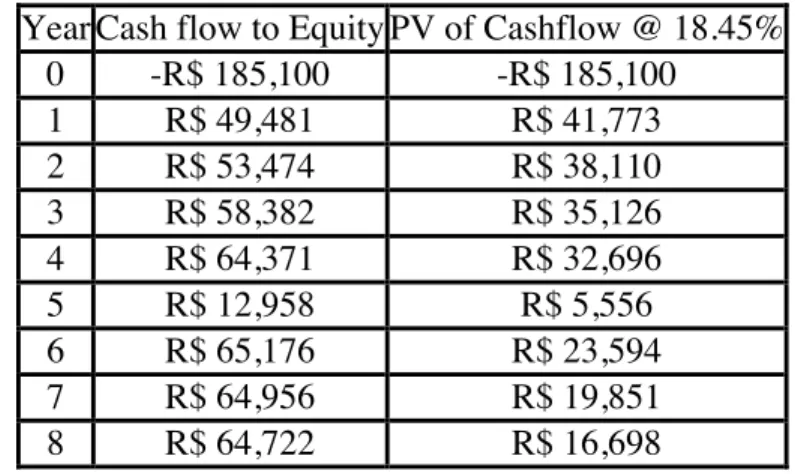
Illustration 5.6: Estimating Cash Flows to Equity for a New Plant: Aracruz
Aracruz Celulose is considering a plan to build a state-of-the-art plant to manufacture linerboard. The plant is expected to have a capacity of 750,000 tons and will have the following characteristics:
1. It will require an initial investment of 250 million BR. At the end of the fifth year, an additional investment of 50 million BR will be needed to update the plant.
2. Aracruz plans to borrow 100 million BR at a real interest rate of 6.3725%, using a ten-year term loan (where the loan will be paid off in equal annual increments). 3. The plant will have a life of ten years. During that period, the depreciable portion of
the plant (and the additional investment in year five), not including salvage value, will be depreciated using double declining balance depreciation, with a life of ten years.6 At the end of the tenth year, the plant is expected to be sold for its salvage value of 75 million BR.
4. The plant will be partly in commission in a couple of months but will have a capacity of only 650,000 tons in the first year and 700,000 tons in the second year before getting to its full capacity of 750,000 tons in the third year.
5. The capacity utilization rate will be 90% for the first three years and rise to 95% after that.
6. The price per ton of linerboard is currently $400 and is expected to keep pace with inflation for the life of the plant.
7. The variable cost of production, primarily labor and material, is expected to be 45% of total revenues; there is a fixed cost of 50 million BR, which will grow at the inflation rate.
8. The working capital requirements are estimated to be 15% of total revenues, and the investments have to be made at the beginning of each year. At the end of the tenth year, it is anticipated that the entire working capital will be salvaged.
9. Aracruz’s corporate tax rate of 34% will apply to this project as well.
6With double declining balance depreciation, we double the straight line rate (which would be 10 percent a
year, in this case with a ten-year life) and apply that rate to the remaining depreciable book value. We apply this rate to the investment in year five as well. We switch to straight line depreciation in the 6th year