Development and Application of a
Finite Volume Method for the Computation
of Flows Around Moving Bodies on
Unstructured, Overlapping Grids
Vom Promotionsausschuss der
Technischen Universit¨at Hamburg-Harburg
zur Erlangung des akademischen Grades
Doktor-Ingenieur
genehmigte Dissertation
von
Hidajet HAD ˇ
ZI ´
C
Bosnien und Herzegowina
Hidajet Hadˇzi´c, 1. Auflage, Hamburg: Arbeitsbereiche Schiffbau, 2006 ISBN 3-89220-633-3
Gutachter: Prof. Dr. Milovan Peri´c Prof. Dr.-Ing. Gerhard Jensen Prof. Dr.-Ing. Heinz Herwig
Tag der m¨undlichen Pr¨ufung: 15.12.2005
c
Arbeitsbereiche Schiffbau
Technische Universit¨at Hamburg-Harburg Schwarzenbergstrasse 95 C
Abstract
In this thesis the development and application of an overlapping grid technique for the nu-merical computation of viscous incompressible flows around moving bodies is presented.
A fully-implicit second-order finite volume method is used to discretize and solve the un-steady fluid-flow equations on unstructured grids composed of cells of arbitrary shape. The computational domain is covered by a number of grids which overlap with each other and can move relative to each other in an arbitrary fashion.
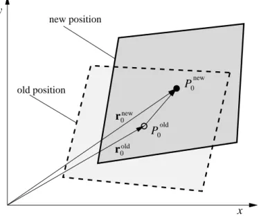
For the treatment of grid movement, besides the standard method which is based on the arbi-trary Lagrangian-Eulerian formulation of the governing equations, a novel method based on the solution of the governing equations in their Eulerian formulation was developed. Thus, instead the computation of grid fluxes, the grid motion is taken into account by appropriate approxima-tion of the local time derivative in the unsteady term of the governing equaapproxima-tions and by adding mass sources/sinks produced by moving walls in the near-wall region. The new method allows the change in grid topology and can be conveniently used with a re-meshing technique.
A special implicit procedure for coupling of the solution on overlapping grids is developed. The interpolation equations used to compute the variable values at interpolation cells distributed along grid interfaces are involved in the global system of linearized equations that arise from discretization. Such a modified linear equation system is solved for the whole domain providing that the solution is obtained on all grids simultaneously. In this way a strong inter-grid coupling characterized by smooth and unique solution in the whole overlapping region and a good con-vergence rate is achieved. The mass conservation, which is violated by interpolation, is enforced by adjusting the interface mass fluxes.
For a successful handling of body motion, the computational cells are allowed to be active or passive, depending on their position relative to the computational domain. The grid cells which are at the current time step outside the computational domain (e.g. covered by a body) are tem-porarily deactivated. These cells are reactivated when they reenter the computational domain. In this way a motion of grid components of arbitrary large scales can be achieved.
The method developed in the present study was verified by applying it to some flows for which either the numerical solution or experimental data were known or the solution could be obtained using another numerical technique available in the commercial software. The accuracy of the method was assessed through the systematical grid refinement. The potential of the pro-posed overlapping grid method and its advantages over other available techniques for handling moving bodies was demonstrated on a number of flows which involve complex and large-scale body motion.
The research for this thesis I performed at Fluid Dynamics and Ship Theory Section of the Tech-nical University Hamburg-Harburg.
I wish to express my gratitude to Professor Milovan Peri´c and Professor Gerhard Jensen for their continuous support, guidance and encouragement throughout this study. I wish also to thank all my colleagues in the Fluid Dynamics and Ship Theory Section with whom I shared many pleas-ant moments and useful discussions, in particular to Muris Torlak and Dr. Eberhard Gerlach. Financial support from the German Academic Exchange Service (DAAD), Technical University Hamburg-Harburg and ICCM GmbH, that made this study possible, is greatly appreciated. My special thanks goes to my family for their love, support and encouragement during all these years.
Contents
1 Introduction 1
1.1 Previous related studies . . . 2
1.2 Present contributions . . . 4
1.3 Outline of the thesis . . . 6
2 Governing Equations 7 2.1 Introduction . . . 7 2.2 Conservation equations . . . 8 2.2.1 Conservation of mass . . . 8 2.2.2 Conservation of momentum . . . 9 2.2.3 Conservation of energy . . . 9
2.3 Generic transport equation . . . 10
2.4 Boundary and initial conditions . . . 11
3 Numerical method 13 3.1 Finite volume method . . . 13
3.2 Discretization procedure . . . 14
3.2.1 Approximation of volume integrals . . . 15
3.2.2 Approximation of surface integrals . . . 15
3.2.3 Convection . . . 16
3.2.4 Diffusion . . . 18
3.2.5 Calculation of gradients at CV center . . . 18
3.2.6 Source terms . . . 20
Treatment of pressure term in momentum equation . . . 20
3.2.7 Integration in time . . . 20
3.2.8 Final form of algebraic equations . . . 22
3.3 Calculation of pressure . . . 23
3.3.1 SIMPLE algorithm . . . 24
Cell-face velocity . . . 24
Predictor stage . . . 24
Corrector stage . . . 25
3.4 Implementation of boundary conditions . . . 26
3.4.1 Inlet boundaries . . . 26 i
3.4.2 Outlet boundaries . . . 27
3.4.3 Symmetry boundaries . . . 27
3.4.4 Wall boundaries . . . 28
3.4.5 Boundary conditions for the pressure-correction equation . . . 28
3.5 Solution procedure . . . 29
3.5.1 Segregated algorithm . . . 29
3.5.2 Under-relaxation . . . 30
3.5.3 Solution of linear equation systems . . . 31
3.5.4 Solution algorithm . . . 31
4 Grid Movement 33 4.1 Introduction . . . 33
4.2 Arbitrary Lagrangian-Eulerian approach . . . 33
4.2.1 Space conservation law . . . 34
4.2.2 Discretization and boundary conditions . . . 36
4.3 Local-time-derivative based approach . . . 37
4.3.1 Near-wall treatment . . . 39
4.4 Assessment of moving grid methods . . . 39
4.4.1 Piston-driven flow in a pipe contraction . . . 40
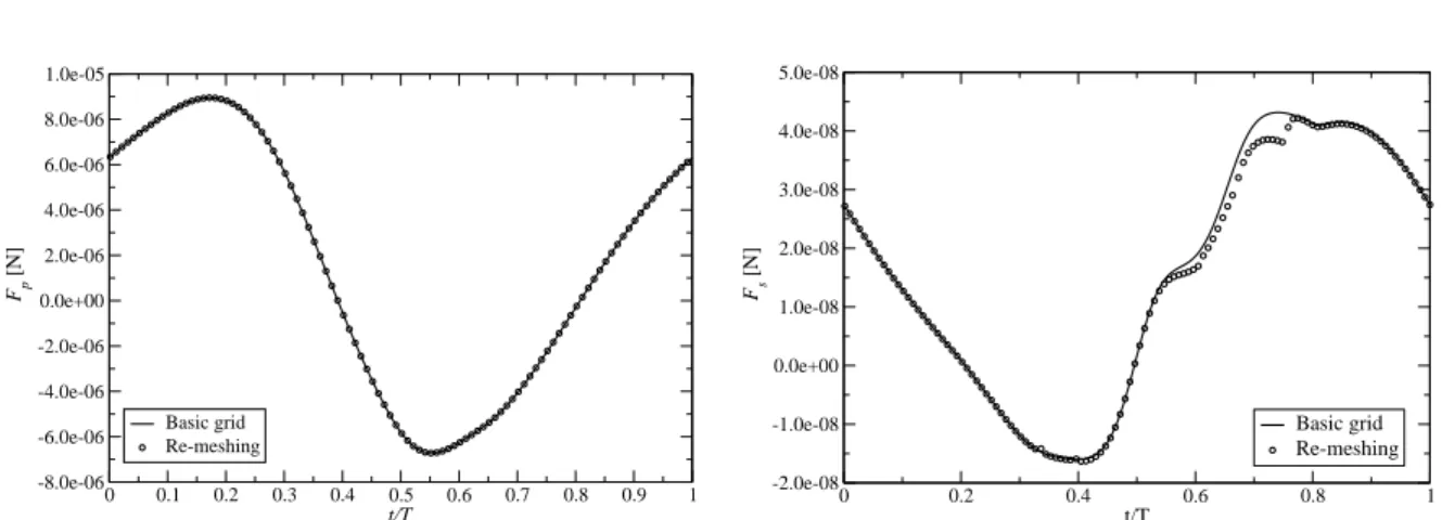
4.4.2 Re-meshing . . . 44
4.5 Concluding remarks . . . 46
5 Overlapping grid technique 53 5.1 Introduction . . . 53
5.2 Outline of overlapping grid methodology . . . 55
5.2.1 Inter-grid communication . . . 56
5.2.2 Accuracy and conservation properties of interpolation . . . 62
5.3 Solving the governing equations on overlapping grids . . . 64
5.3.1 Treatment of inactive cells . . . 64
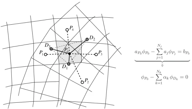
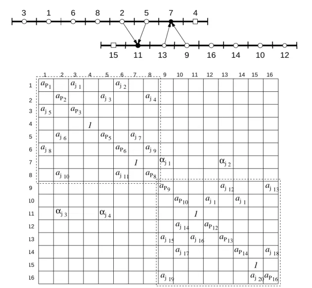
5.3.2 Coupling of the solution on overlapping grids . . . 66
5.3.3 Mass conservation . . . 69
5.3.4 Cell-face values at interfaces . . . 74
5.3.5 Treatment of moving overlapping grids . . . 75
5.4 Solution procedure . . . 75
6 Verification and application of the method 79 6.1 Flow around a circular cylinder in a channel . . . 79
6.1.1 Influence of the cylinder grid . . . 87
6.1.2 Conservation errors . . . 88
6.2 Lid-driven cavity flow . . . 88
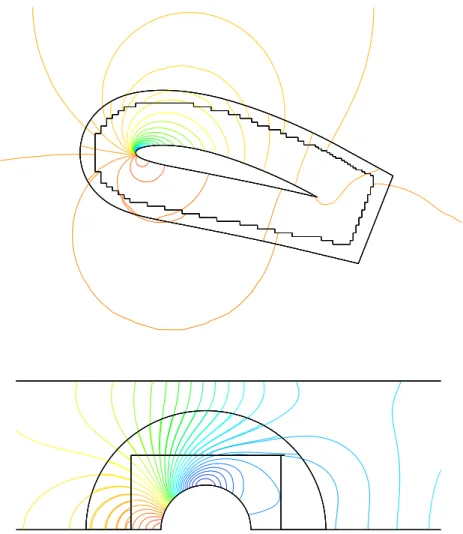
6.3 Flow around a NACA 4412 airfoil . . . 97
6.4 Flow around rotating plate in a channel . . . 100
CONTENTS iii
6.6 Flow in a mixer . . . 108
6.7 Flow around the Voith-Cycloidal-Rudder . . . 111
6.7.1 Problem definition . . . 111
6.7.2 Numerical grid and boundary conditions . . . 112
6.7.3 Results . . . 114
7 Conclusions and outlook 121
A Interpolation functions 125
B SST turbulence model 127
References 129
C
HAPTER
1
Introduction
The numerical solving of the mathematical model which describes the fluid flows, known as Computational Fluid Dynamics (CFD), is nowadays increasingly becoming a design tool in var-ious parts of industrial product development. Numerous examples include flow around a car or a ship or flow in an internal combustion engine etc. This is a field of large expansion mainly due to the progress in computer technologies and the computational algorithms.
Fluid flows involving relative motion between device components is an important class of problems which require advanced computational techniques for their simulation. There are many important applications of this kind such as flying or/and floating bodies, rotating machinery (in particular extruders, mixers, pumps, propellers), approaching/diverting objects (e.g. car overtak-ing), navigation devices (rudders, flapping wings), fluid-solid interaction, etc. These examples cover a wide range of flow regimes and component sizes, and they all have in common the fact that both the flow fields and geometries are complex. Understanding the unique unsteady flow features associated with moving bodies is crucial for design purposes. Therefore, accurate and ef-ficient solution methods for such flows are required. Due to continuous development in computer hardware (increase of both, the speed and the memory) and the progress in CFD techniques, nu-merical simulations of such problems have become feasible. However, the computational costs are still quite considerable because the moving bodies greatly increase the complexity of the problem.
The main characteristic of industrial applications is the geometrical complexity of the solu-tion domain. Therefore, the use of unstructured meshes for computasolu-tional fluid dynamics prob-lems has become widespread. The main reason for this is the ability of unstructured meshes to discretize arbitrarily complex geometrical domains and the ease of local and adaptive grid refine-ment which enhances the efficiency of the solution as well as solution accuracy. In parallel, so-lution algorithms for computing flows on unstructured grids have been continuously developed. Among a number of discretization methods available, the finite volume methods are most widely used for engineering CFD applications. This is mostly due to the inherent conservativeness and ease of understanding, development, and use of such methods. These methods are capable to ac-commodate arbitrary polyhedral grids composed of cells of different topology. Such grids have gained recently popularity because of the improved efficiency and accuracy over pure tetrahedral
grids. For a successful simulation of flows around moving bodies, the discretization in time plays a key role, both from the efficiency and accuracy point of view. Due to prohibitively low time-step limitations of explicit schemes, implicit time-integration algorithms are usually preferred.
To compute flows around moving bodies, the numerical grid needs to be adapted to the mov-ing body and therefore move with it. Special treatment is required for the governmov-ing equations to account for grid movement. The commonly used approach is to use the definition of the gov-erning equations in a moving frame of reference – the so called arbitrary Lagrangian-Eulerian (ALE) formulation. Methods that use moving grids are well established in commercial software. However, there are problems when bodies move relative to each other in an arbitrary manner. Large motion leads inevitably to high grid distortions and, due to pure mesh quality, the use of a single domain-fitted grid of specified topology becomes no longer possible. These problems could be overcome by introducing re-meshing and/or overlapping grids. Commercial codes do not offer such features1.
1.1
Previous related studies
A number of numerical techniques to handle fluid flows involving moving bodies have appeared over the last two decades. The three major ones are: i) the grid deformation approach, ii) the grid re-meshing approach, iii) the overlapping grid approach.
In the grid deformation approach, the computational grid around a moving body is ”adjusted” at each time step such that it conforms to the new position of the body. The grid topology and the total number of control volumes are preserved. It has been used in conjunction with structured grids [21] as well as with unstructured grids [5]. The advantage of this approach is that the flow solver can be easily made fully conservative. The disadvantage of this approach is that the scale of the motion of a moving body cannot be large in comparison to the body size and usually the rotations are not allowed. The scale of the body motion can be increased and the rotation can be achieved by using so called sliding grids. In that case a part of the grid is attached to body and moves with it, while the remaining part of the grid is stationary. Between the fixed and the moving part of the grid there is a sliding interface, which is a predefined surface (usually plain, cylindrical or spherical surface). Combining the grid deformation with sliding grids a higher level of body motion can be achieved [30], but it is still limited by the grid deformation and by sliding interfaces which require a common interface (allow no overlapping) between moving and stationary grid blocks.
In the grid re-meshing approach, the grid near the moving body is regenerated at each time step according to the new position of the body. This approach eliminates the limitation on grid topology and thus grid quality around the moving body can be maintained. Furthermore grid mo-tions of arbitrary scales are possible. The main drawback of this approach is that flow variables
1Only recently, shortly before finishing-up the thesis, one commercial CFD software provider announced the
1.1. Previous related studies 3
must be interpolated from the old to the new grid at each time step and it is not easy to interpolate the flow variables in the conservative manner. Another drawback is that the grid has to be gen-erated many times which is a time consuming and expensive operation. Usually, the re-meshing is combined with the grid deformation so that the grid is deformed while the body moves for a certain distance which is followed by a re-meshing [46]. Another possibility is to consider only a part of the grid in immediate vicinity of the body for the movement and re-meshing, while the rest of the grid remains stationary [94].
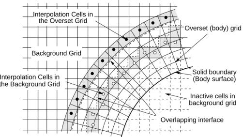
The previous two approaches fall in the category of domain-conforming grid methods, in which a single grid or several grid blocks which do not overlap with each other cover the com-putational domain. In the overlapping grid approach, also called Chimera grid approach, the computational domain is covered by a number of overlapping grids. Grid components associated with moving bodies move with the bodies while the other grid components remain stationary. The component grids are not required to match in any special way, but they have to overlap suf-ficiently to provide the means of coupling the solutions on each of them. This method allows the component grids to move relative to each other in an arbitrary fashion, making them perfect for use in applications with moving bodies. Grid adjustments or grid regeneration are thus not necessary2. The grid components are usually geometrically simple and allow for independent
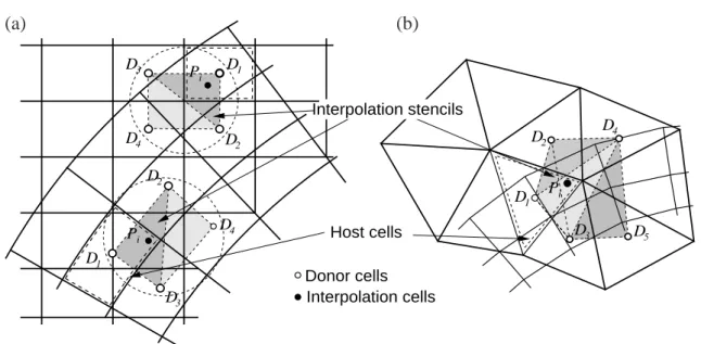
griding of higher quality than would be possible in the case of a single grid. Flow variables are interpolated between the overlapped grids to exchange the information; however, the interpola-tion takes place only in a limited number of cells distributed along grid interfaces rather then in the whole domain, as is the case in re-meshing approaches. The grid interfaces can be placed in regions where the variables vary more smoothly than in the vicinity of the body, thus making interpolation errors smaller. The major drawback of this approach is that it is difficult to ensure conservation of the computed variables/quantities across grid interfaces.
Obviously for applications with bodies moving in an arbitrary fashion and involving large-scale body motion, the first above-mentioned technique is not quite suitable due to limitations imposed on the level of grid deformation and the shape of sliding interfaces. Among other two techniques, the overlapping grid approach offers more flexibility and has the following two im-portant advantages over the re-meshing technique: i) no requirement for grid re-generation, ii) possibility to achieve a better grid quality since the boundary of the overlapping grids can be arbitrarily chosen.
The overlapping grid approach has been used by a number of authors in the past. It has been applied mostly with structured grids. The first overlapping grid computations were performed by Starius who solved elliptic and hyperbolic problems [72, 73]. Steger et al.[75] and Benek
et al.[8] used the overlapping structured grids for computation of flows in complex geometries.
A review article about overlapping grid computations in gas dynamics presenting a number of
2Under assumption that the bodies do not deform. If this is not the case, the grid around the body needs to be
adapted. Usually the deformation of the body is small so that the grid can be adjusted without changing its topology (grid deformation approach).
applications in complex steady geometrical configurations and with multiple moving bodies is given by Steger and Benek [74]. Further applications of the overlapping grids to problems with moving bodies are presented in references [23, 48]. Recently, the overlapping grid techniques have been used also with unstructured grids. A few publications appeared which present the overlapping grid methods for unstructured tetrahedral grids [55, 44]. A more detailed review of publications related to overlapping grid techniques will be given later in chapter 5.
The main objective of the present research was to develop a method for computation of flows around moving bodies using the overlapping grid technique and arbitrary unstructured meshes. The unstructured meshes are preferred due to reasons mentioned above. The limitations of structured grids concerning the grid topology and controlling of the grid resolution can thus be overcome. Although, in general, a set of structured overlapping grids can be used to cover the domains of a high level of complexity, the complexity of such overlapping grid systems in-creases significantly due to the increasing number of component grids required. Combination of unstructured and overlapping grids provides an optimum in the treatment of problems with moving bodies. The highest flexibility can be achieved in both treatment of complex geometry and grid motion, while the complexity of the overlapping grid systems can be kept at low level since the number of overlapping grid components required is much smaller in comparison to structured grids.
When the ALE approach is used for treatment of grid movement, in most instances the ef-fort has to be made to ensure that the grid movement itself does not influence the flow field3. To ensure this the so called space conservation law (SCL) has to be satisfied [20]. On arbitrary polyhedral unstructured grids the enforcement of the space conservation law may become diffi-cult due to complex grid structure. Furthermore, the application of re-meshing is also diffidiffi-cult due to data transfer between two grids of different topology.
Another concern of the present study was to investigate the possibility of the treatment of the grid movement in an alternative way which would be easier for implementation on arbitrary unstructured grids and would facilitate the implementation of the re-meshing technique. The overall method would thus have no restrictions regarding the complexity of solution domains and body motion. For the sake of simplicity but without loss of generality, development has been performed in two spatial dimensions. The extension to three-dimensional flows is straightforward and the necessary steps are explained were appropriate.
1.2
Present contributions
The major contributions of the present work can be summarized as follows:
• A new discretization and solution practice that uses a fully-implicit method and approx-imation of local time derivative in the Eulerian formulation of the governing equations,
3It has to be ensured that no artificial flow appears due to grid motion. A convenient test case is a uniform stream
1.2. Present contributions 5
rather than the space-conservation law and the grid velocity in the arbitrary Lagrangian-Eulerian (ALE) formulation, for the treatment of the grid movement has been developed. It was shown that the treatment of the grid movement in such a way produces results of comparable accuracy as the conventional ALE approach, while offering some advantages over the ALE method, especially on arbitrary unstructured grids. Namely, the variable values at specified points (centers of control volumes), required for approximation of the local time derivative, are much easier to compute and can be computed independently of the grid topology. On the other hand, the computation of grid velocities (enforcement of the space conservation low) for unstructured grids composed of cells with arbitrary num-ber of cell-faces may be very complicated. Another very important feature of this new technique is that it allows the change of the grid topology during the computation, making the method suitable for application with re-meshing technique.
• The re-meshing technique as a special case of the moving grid has been incorporated in the spirit of the new discretization technique. Interpolation of the dependent variables at the control-volume centers from the old to the new grid was shown to be enough for continuation of the computation after re-meshing. The accuracy was also found to be not significantly affected by the data transfer.
• An overlapping grid technique based on a finite volume discretization on arbitrary un-structured grids has been developed. A special implicit technique for the treatment of grid interfaces, based on the simultaneous solution of interpolation equations in the global lin-ear equation system, was developed. It is shown that such a treatment provides a strong inter-grid coupling and smooth and unique solution over the whole computational domain and achieves a convergence rate in the range of comparable single grids. The method is applicable to stationary as well as moving overlapping grids and allows a nearly arbitrary large scale motion between the grid components providing an efficient tool for handling of moving bodies.
• Due to Neumann boundary conditions imposed on the pressure-correction equation when the mass flow rate over the boundaries is given, the strict mass conservation is essential for the solution of this equation. Since the interpolation technique used for the solution cou-pling between overlapping grids is not strictly conservative, additional treatment is neces-sary to fulfill this requirement. Two possible techniques to enforce the mass conservation were examined here, and the strategy based on the global correction of interface fluxes was adopted. It was shown that this global correction also provides the mass conservation on each grid as the converged solution is approached, as expected due to flow field continuity.
• The present method is embodied in a computer program for two-dimensional problems in a general way appropriate for the use of grids of arbitrary topology. The performance and accuracy of the method was first extensively assessed on a number of flows for which the reference solutions exist. The flexibility of the overlapping grid technique was clearly demonstrated on a number of flows which involve moving bodies with large scales of body motion.
1.3
Outline of the thesis
The thesis is subdivided into seven chapters. Chapter 2 summarizes the conservation equations governing the incompressible fluid flow. The equations are given in their integral form suitable for the discretization method used for their solution. A generic transport equation for an arbitrary scalar variable is introduced as a model equation upon which the discretization technique is derived.
The subsequent three chapters consider different aspects of the numerical methodology con-cerning the discretization of the governing equations, treatment of the grid movement and over-lapping grids technique. Chapter 3 presents the second-order finite volume discretization method applicable to unstructured meshes of arbitrary topology. The discretization of the generic trans-port equation for a scalar variable is described term by term. This is followed by the derivation of a pressure-correction equation, which is used for resolving the velocity-pressure coupling and calculation of pressure. Finally, a segregated solution approach for the coupled system of equations along with steps required to obtain the solution is outlined.
In chapter 4 two methods for the grid movement implemented in the present study are de-scribed. First the method based on the Lagrangian-Eulerian formulation of the governing equa-tions and the use of the space conservation law is outlined. Then the novel method based on the approximation of the local time derivative at the fixed location in space is described. The accuracy and performance of both methods is assessed on a piston-driven flow in a pipe contrac-tion. In addition, the new method for grid movement is tested in combination with re-meshing technique.
Chapter 5 presents the overlapping grid technique developed in the present study. First, an outline of the overlapping grid technique is given, followed by description of the algorithms for hole cutting and donor searching adopted in this study. Next the methodology for the solution of governing equations on overlapping grids is explained, with special emphases on inter-grid cou-pling. An implicit method is developed, which provides strong inter-grid coupling and smooth and unique solution across overlapping interfaces. The necessity of the mass conservation is also discussed and two possible approaches to enforce the mass conservation on overlapping grids are described.
In chapter 6 the present method is assessed on a number of examples for which either bench-mark numerical solutions or experimental data are available or the solution could be obtained with another technique available in the commercial software. Special attention is paid to the assessment of the overall accuracy, grid coupling and conservation errors caused by inter-polation of the solution between overlapping grids. In addition predictions are given of some complex flows involving multiple moving bodies for which no experimental or numerical data are available. These computations are shown in order to demonstrate the flexibility and the range of applicability of the overlapping grid method in computation of flows around moving bodies.
Finally, conclusions drown from the studies performed in this thesis and suggestions for future work are given in chapter 7.
A CD-ROM with a number of animations presenting the results of computation of flows around moving bodies is attached.
C
HAPTER
2
Governing Equations
This chapter contains an overview of the equations governing the incompressible Newtonian fluid flow. The conservation equations for mass, momentum and energy are used in their integral form as the mathematical basis for the numerical method adopted in this study. The conservation equations are given in the coordinate-free form and the momentum equation is resolved in terms of Cartesian vector components. A generic conservation equation for an arbitrary scalar variable is introduced as a model equation upon which the discretization procedure is derived. Finally, the boundary and initial conditions necessary for completion of the mathematical model are discussed.
2.1
Introduction
The derivation of basic equations of fluid dynamics is based on the fact that the dynamical be-havior of a fluid is determined by the conservation laws of mass, momentum and energy. The conservation of a certain flow quantity means that its variation inside an arbitrary control vol-ume can be expressed as the net effect of the amount of the quantity being transported across the boundary by convection and diffusion and any sources or sinks within the control volume. The fluid is regarded as continuum, which assumes that the matter is continuously distributed in space. The concept of continuum enables us to define velocity, pressure, temperature, density and other important quantities as continuous functions of space and time. In addition, special mathe-matical tools (such as field theory) for the analysis of the problems of continuum mechanics can be used.
In the derivation of the governing equations of fluid dynamics the Eulerian or control
vol-ume approach is conveniently used, rather then Lagrangian or material approach. The formal
derivation of equations follows from the Reynolds’ transport theorem1 [92] which facilitates the implementation of laws and principles concerning the behavior of a system (made of the same fluid particles) in an arbitrary control volume.
1Also called the generalized transport theorem [70].
2.2
Conservation equations
In this section the conservation equations of mass, momentum and energy for an arbitrary control volumeV fixed in space2bounded by a closed surfaceS, (see figure 2.1), will be presented.
x y z S rP V d s P
Figure 2.1: Arbitrary control volumeV.
2.2.1
Conservation of mass
The conservation equation for mass or the continuity equation, for a control volume states that the rate of change of the mass inside the control volume V is equal to the difference between inflow and outflow mass fluxes across the volume surface S. In integral form the continuity equation reads: ∂ ∂t Z V ρdV + I S ρv·ds= 0, (2.1)
where, ρ is the fluid density and v is the fluid velocity. Note that if the fluid is regarded as incompressible, which is the case in this study, the first term on the left-hand side in equation (2.1) is zero since the density is constant. However, for problems with moving grids, which involve changes of the control volume, this term might be considered depending on the numerical method employed (see chapter 4).
2The equations for a moving control volume in conjunction with different solution methods are considered in
2.2. Conservation equations 9
2.2.2
Conservation of momentum
The conservation equation for momentum states that the total variation of momentum, repre-sented by the time variation of momentum within the control volume and the transfer of momen-tum across the boundary of the control volume by fluid motion (called convection or advection), is caused by the net force acting on the fluid in the control volume. In the integral coordinate-free form this equation reads:
∂ ∂t Z V ρvdV + I S ρvv·ds= I S σ·ds+ Z V ρfbdV , (2.2)
whereσ is the stress tensor representing the surface forces and fb represents the vector of body
forces acting on the fluid. The stress tensor can be expressed in terms of basic dependent vari-ables and for Newtonian incompressible fluids is defined as:
σ =µ hgrad v+ (grad v)Ti−pI, (2.3)
wherepis the pressure,µis the dynamic viscosity of the fluid and I is the unit tensor.
In order to be solved, the vector equation (2.2) has to be resolved into specific directions resulting in three equations in terms of vector components. In this study the Cartesian coordi-nate system is used, resulting in the simplest form of momentum equations and insuring strong conservation of momentum components [18, 59]. Substituting equation (2.3) into equation (2.2) and taking dot product with the Cartesian base vector ii, the corresponding equation for the ith
Cartesian component is obtained:
∂ ∂t Z V ρuidV + I S ρ uiv·ds = I S µgradui·ds+ I S µhii·(grad v)T i ·ds − I S pii·ds+ Z V ρfbidV , (2.4)
where ui stands for the ith velocity component and fbi stands for ith component of the body
force.
2.2.3
Conservation of energy
The underlying principle upon which the energy equation is derived, is the first law of thermo-dynamics. It states that any changes in time of the total energy inside control volume are caused by the rate of work of forces acting on the volume and by the net heat flux into it. This equation in its most general form contains a large number of influences whose importance depends on the problem considered. For most engineering flows the energy equation can be written in term of specific enthalpy as:
∂ ∂t Z V ρhdV + I S ρhv·ds= I S q·ds+ Z V (σ :grad v+qT) dV , (2.5)
wherehis the specific enthalpy, q is the heat flux vector andqT is the heat source or sink. If the
fluid is considered to be thermally perfect, specific enthalpy depends only on temperature via the following relation:
h=cpT , (2.6)
where,cpis the specific heat at constant pressure andT is the temperature. The heat flux vector
is related to the temperature gradient by the Fourier’s law:
q=−kgradT , (2.7)
where the proportionality coefficientkis the thermal conductivity of the fluid.
Introducing equations (2.6) and (2.7) into equation (2.5), the energy equation can be re-written in term of temperature as:
∂ ∂t Z V ρcpT dV + I S ρcpT v·ds= I S q·ds+ Z V (σ :grad v+qT) dV . (2.8)
2.3
Generic transport equation
Conservation equations presented above describe the laminar flow of an incompressible New-tonian fluid. In some situations additional processes take place and besides the basic equations some additional transport equations have to be solved. An example is the Reynolds-averaged modeling of turbulent flows, where a number of additional transport equations for turbulent quan-tities have to be solved3. The turbulent quantities may even have vector or tensor character but
can be expressed via a certain number of non-zero components. In addition, equations describing transport of chemical species may be introduced. In general, such equations for the transport of a generic scalar variableφcan be written in the following form:
∂ ∂t Z V ρφdV + I S ρφv·ds= I S Γφgradφ·ds+ I S qφS ·ds+ Z V qφV , (2.9)
whereφstands for the transported variable,Γφis the diffusion coefficient andQφSandQφV stand
for the surface exchange terms and volume sources, respectively. It is important to note that the momentum and energy equations can also be written in the form of equation (2.9). This fact significantly facilitates the numerical procedure since, from the numerical point of view, only one equation has to be discretized4. Equation (2.9) is therefore used as the generic equation for
deriving the numerical procedure described in the next chapter.
3Depending on the model used, additional terms appear in the Navier-Stokes equations. 4For a segregated solution algorithm, which is also adopted in this study.
2.4. Boundary and initial conditions 11
2.4
Boundary and initial conditions
In order to obtain the solution of the governing equations, the initial and boundary conditions have to be specified. Boundary conditions in fluid flow problems are conveniently divided ac-cording to the physical meaning of boundaries like wall, inflow, outflow, symmetry etc. Whatever boundaries appear in a specified problem, the initial and boundary conditions have to be selected so that the problem to be solved is well posed, i.e. the solution exists and depends continuously upon them.
Due to the parabolic nature of the unsteady equations, one set of initial conditions has to be specified. An initial distribution of all dependent variables at the initial instant of time, t =t0,
have to be prescribed in the whole computational domainV:
φ(r, t0) = φ0(r), r
∈V . (2.10)
The governing equations have an elliptic character in space. Therefore, boundary conditions have to be specified at all times and at all domain boundariesSB. Different type of boundaries
require different boundary conditions to be applied. All of them can be classified into two groups:
• Dirichlet boundary condition, when the value of a dependent variable at the portion of the boundarySD
B of the solution domain is specified, e.g.
φ(rB, t) = fj(t), rB ∈SBD. (2.11)
• Neumann boundary condition, when the gradient of a dependent variable at the portion of the boundary of the solution domainSN
B is specified, e.g.
gradφ(rB, t) =fj(t), rB ∈SBN . (2.12)
The implementation of boundary conditions within the numerical method adopted in this study is described in detail in the next chapter.
C
HAPTER
3
Numerical method
In this chapter the finite volume method (FVM) adopted in the present study for solving the con-servation equations presented in the previous chapter is described. It is based on a second-order accurate spatial discretization which accommodates unstructured meshes with cells of arbitrary shape. In addition a fully implicit integration in time is used for the solution of unsteady prob-lems. Computational points are located in the cell center and a collocated variable arrangement is used. A segregated solution procedure is employed to solve the resulting set of non-linear algebraic equations. It leads to a decoupled system of linear algebraic equations for each de-pendent variable. The linearized equation systems are solved using a conjugate gradient solver. The SIMPLE algorithm, leading to an equation for the pressure correction, is used to establish the pressure-velocity coupling and calculate the pressure. Finally the implementation of various boundary conditions is discussed and solution algorithm is outlined.
3.1
Finite volume method
There exists a vast number of methods for the numerical solution of the governing equations. Most of them follow closely the path consisting of the following three steps:
• Space discretization, consisting of defining a numerical grid, which replaces the
contin-uous space with a finite number of discrete elements with computational points at their centroids. At those points the solution of dependent variables are computed. This process is termed grid generation.
• Time discretization, which assumes the division of the entire time interval into a finite
number of small subintervals, called time steps.
• Equation discretization, which is the replacement of the individual terms in the governing
equations by algebraic expressions connecting the variable values at computational points in the grid.
In the present study the finite volume method of discretization is adopted. It utilizes directly the conservation laws, i.e. the governing equations are discretized starting from their integral
form. The solution domain is discretized by an unstructured mesh composed of a finite number of contiguous control volumes (CVs) or cells. Each control volume is bounded by a number of cell faces which compose the CV-surface and the computational points are placed at the center of each control volume. There is no restriction in the shape that the control volumes may have, i.e. an arbitrary polyhedral shape is allowed (see figure 3.1). This is achieved by a special data structure based on cell faces, which provides the data connectivity between the cells sharing the same cell face. It makes the flow solver capable to deal with meshes consisting of cells of different topology (e.g. hybrid meshes) since the number of cell faces per CV can vary arbitrarily from one CV to another. The same data structure supports also the local (cell-wise) grid refinement since only the list of cell faces needs to be updated. The interface between refined and non-refined cells can, thus, be treated fully conservatively. All this provides a great flexibility regarding the numerical mesh that can be used.
The collocated (non-staggered) variable arrangement, which is suitable for the arbitrary un-structured meshes, is used. It assumes that all dependent variables share the same control volume. Equations are solved in a Cartesian coordinate system, providing the strong conservation form of the momentum equations [18] and making the method insensitive to the grid non-smoothness [59]. The system of conservation equations is treated in the segregated way, meaning that they are solved one at a time, with the inter-equation coupling treated in the explicit manner. Before solving, each equation is linearized and the non-linear terms are lagged. An iteration procedure is employed to handle the non-linearity and inter-equation coupling.
P P P z x y 0 P s1 1 j n sn sj rP 0 dj
Figure 3.1: A general control volume of arbitrary shape.
3.2
Discretization procedure
The discretization procedure will be demonstrated for a generic transport equation (2.9). The same procedure is followed to obtain the discrete counterparts of all governing equations. Only
3.2. Discretization procedure 15
the discretization of the continuity equation is described separately. In the present method, the continuity equation is utilized to compute the pressure. The derivation of a pressure-correction equation, used to obtain the pressure, and its discretization is described in section 3.3.
When equation (2.9) is integrated over a CV shown in figure 3.1, it attains the following form: ∂ ∂t Z ∆V ρφdV | {z } Rate of change + N X j=1 Z Sj ρφv·ds | {z } Convection = N X j=1 Z Sj Γφgradφ·ds | {z } Diffusion + N X j=1 Z Sj qφS ·ds | {z } Surface source + Z ∆V qφV dV | {z } Volume source .(3.1)
The surface integrals in equation (2.9) are here represented as a sum of integrals over a number of cell faces defining the cellP0. Equation (3.1) has four distinct parts: rate of change (transient
or unsteady term), convection, diffusion and sources. The discretization of each particular term in equation (3.1) is described in the following subsections.
3.2.1
Approximation of volume integrals
The volume integrals in equation (3.1) are approximated by the mid-point rule, which is second-order accurate for any CV shape. The mean value of the integrated variable is approximated by the value of the function at the CV centerP0,
ΨP0 = Z
∆V
ψdV =ψ ∆V ≈ψP0 ∆VP0. (3.2)
Since the variable value at the CV center, needed for the calculation of the integral, is readily available (variables are stored at CV centers), no additional approximations are required.
3.2.2
Approximation of surface integrals
The surface integrals are also approximated by mid-point rule, thus
Fj =
Z
Sj
f ·ds≈fj ·sj, (3.3)
whereFj represents the flux of the transported variable across the cell facej andf is the flux
vector, see equation (3.1). Unlike in volume integrals, the variable values at cell-face center required for the calculation of surface integrals are not directly available. They have to be evalu-ated using additional approximations. In order to retain second-order accuracy of mid-point rule approximation for integrals, the cell-face value has to be evaluated with at least a second-order accuracy.
3.2.3
Convection
Using the mid-point rule, the convective flux through the cell facej is approximated as
Fc
j =
Z
Sj
ρφv·ds≈φjm˙j, (3.4)
whereφjis the value of the variableφat the cell-face center andm˙j is the mass flux through the
cell facej. The later is assumed known, it is computed using values from the previous iteration according to the simple Picard-linearization procedure [26]. The value ofφat the cell-face center has to be computed by interpolation from cell-center values. The methods used in this study are described below.
Central differencing scheme (CDS)
There are many possibilities to interpolate variables at cell-face center. One of the simplest is the linear interpolation, which provides the second-order accuracy. Using linear interpolation the value at pointj′ (figure 3.2), which lies at the line connecting two cell centers, is obtained as:
φj′ =φPjλj+φP0(1−λj) , (3.5)
whereλj is the interpolation factor calculated as
λj =
(rj−rP0)·dj dj ·dj
. (3.6)
Here dj = rPj − rP0 is the vector connecting the point P0 with its neighboring point Pj (see figure 3.2). This approximation is second-order accurate at the locationj′. Ifφ
j′ is used instead of
φj in equation (3.4) a first order error term is introduced which depends on the distance between
j andj′. If pointj′lies close to the pointj, the first order error term is small and the accuracy of the integral approximation will not be affected significantly. On the other hand, ifj′ is far from cell-face centerj, the accuracy of the integral approximation may be impaired. In such a case, the second-order accuracy can be recovered by applying a correction as follows (see figure 3.2):
φj =φ′j+ (gradφ)j′(rj −rj′). (3.7)
The gradient atj′ is obtained by interpolating the gradients from the two CV centers according to equation (3.5). The gradients at CV center have to be calculated anyway for the evaluation of diffusive fluxes through CV faces and also in some cases to compute source terms.
Linear interpolation described here is usually referred to as central-differencing scheme (CDS), since it leads to the same results as the use of central differences for the first derivatives in finite-difference methods.
Although the CDS is very simple and has the desired accuracy (second-order accurate) it may, in certain circumstances (e.g. high value of the local Peclet number or in computations of turbulent flows [28]), produce non-physical oscillatory solutions. Therefore, a method that provides necessary stability is required.
3.2. Discretization procedure 17 P 0 P sj dj j j j’
Figure 3.2: Linear interpolation at cell-face center.
Upwind differencing scheme (UDS)
A widely used scheme, which guarantees bounded (non-oscillatory) solutions is the upwind
differencing scheme (UDS). It assumes zero order polynomial approximation between the two
neighboring cells. The value ofφ at cell-face center is approximated by the value at CV center on the upwind side of the face, i.e.
φj =
(
φP0 if m˙j ≥0,
φPj if m˙j <0.
(3.8) UDS is bounded and unconditionally stable, i.e it will never produce oscillatory solutions. How-ever, these properties have been achieved by sacrifying accuracy. Since it is only first-order accurate, UDS was found to be numerically diffusive, requiring a very fine grid resolution to achieve acceptable accuracy.
Blending of two schemes
To recover the lost accuracy and at the same time to maintain the boundedness, the second-order CDS approximationφcdsj can be blended with some amount of the first-order UDS approximation
φudsj . The value at the cell face is then calculated as:
φj =φudsj +γ φcds j −φ uds j old , (3.9)
whereγ is the blending factor with a value between zero and unity. The amount of CDS scheme can be controlled by choosing an appropriate value of the blending factor. In some cases it may be necessary to use some lower values ofγ in order to suppress oscillations near discontinuities or peaks in profiles when the grid is too coarse. On the other hand, more upwind, i.e. lower value
of blending factor may impair the accuracy [56]. It is, therefore, recommended to use the values of the blending factor as close to unity as possible. One can seek an optimum between stability and accuracy.
Equation (3.9) is implemented using the so called deferred correction approach [59]. Only the first term on the right hand side in equation (3.9), which comes from UDS, contributes to the coefficient matrix, ensuring that the contributions to the coefficients are unconditionally positive (see section 3.2.8). The second term which presents the difference between CDS and UDS approximation is treated explicitly. This term is calculated using the values from the previous iteration. Many other possibilities to computeφj exist; see reference [26] for further details.
3.2.4
Diffusion
Using the mid-point rule, the diffusive fluxFD
j through the cell facejcan be calculated as:
FD j = Z Sj Γφgradφ·ds≈Γφj (gradφ)∗j ·sj = Γφj ∂φ ∂n ! j Sj, (3.10)
where Γφ is the diffusion coefficient and Sj is the area of cell face. In order to calculate the
diffusion flux, an approximation of the derivative at the CV face in the direction normal to the cell face is required. This quantity could be computed by interpolation of cell-center gradients to the cell-face center. Cell-center gradients are calculated explicitly using one of the approximations described in section 3.2.5. Since the simple interpolation may lead to oscillations (see [26] for details), another approximation suggested by Muzaferija [54], which prevents oscillations and retains second-order accuracy, is used:
∂φ ∂n ! j ≈ φPj−φP0 |dj| − (gradφ)old j · dj |dj| − sj |sj| ! , (3.11)
where the value of(gradφ)old
j is calculated by interpolation using equation (3.5). The first term
on the right-hand side represents a central-difference approximation of the derivative in the di-rection ξ of a straight line connecting nodes P0 and Pj (see figure 3.2). This term is treated
implicitly, i.e. it contributes to the matrix coefficients. The second term which corrects the error due to the fact that we need the derivative in the direction of cell-face normal n (figure 3.2) is calculated using previous values of the variables and treated explicitly, i.e. added to the source term.
3.2.5
Calculation of gradients at CV center
The gradient at CV-center can be easily calculated using Gauß’ theorem and mid-point rule approximation as follows: Z V gradφdV = I S φds ⇒ (gradφ)P0 ≈ P jφj sj ∆VP0 . (3.12)
3.2. Discretization procedure 19
This approximation is second-order accurate and is applicable to cells of arbitrary shape, which makes it useful in conjunction with unstructured grids.
Another possibility to calculate gradients at the CV center with second-order accuracy is based on linear shape functions. Assumption of a linear variation of the dependent variableφin the neighborhood of pointP0(including pointsPj) leads to the following set of equations:
dj·(gradφ)P0 =φPj−φP0 (j = 1, ..., Nj), (3.13)
where dj = rPj −rP0 is the vector connecting point P0 with its neighborPj (see figure 3.2). The unknown gradient vector is obtained by solving this system of equations which is over-determined since the number of neighboring points Pj involved in equation (3.13)1 is always
grater then the number of the unknown vector components2. The system (3.13) is solved by
means of a least-squares method and the unknown gradient vector is computed as:
(gradφ)P0 =D −1X
j
dTj(φPj −φP0), (3.14)
where matrixDis calculated as
D=X
j
dTjdj. (3.15)
Note that the matrixDis symmetric3and its coefficients depend solely on the grid geometrical
properties and hence a single evaluation ofD−1 is necessary for a given grid.
In this study both methods have been incorporated and tested. It was found that, on irregular grids with strong non orthogonality (like e.g. triangular grids), the second method based on shape functions produces more accurate results. If the method based on Gauß’ theorem is used on such grids, cell-face values in equation (3.12) should be calculated using equation (3.7). This, however, requires iterations since the values of gradients needed for interpolation are still not available and have to be computed. Numerical tests have shown that a few iterations (typically 3-5) are enough to recover the accuracy. But the least-squares method still remains more accurate and, therefore, may be recommended to be used for calculation of gradients. One, however, needs to be careful, since the least square method does not perform well in computations with complex turbulence models (like Reynolds’ stress models). In such cases it may even cause serious convergence problems [29]. Our experience has also shown that the least-square method may lead to divergence on grids with a high aspect ratio, which evolve e.g. in the near-wall region in computations with low-Returbulence models. This may be put in touch with explanation in [53] that on strongly distorted grids matrixDin equation (3.15) can become singular and thus lead to divergence of the solution process.
1The number of points is equal to the number of cell faces enclosing the cellP
0. For boundary faces, points
which lie at the boundary are included in equation (3.13).
2Minimal number of cell faces surrounding a CV is3in 2-D and4in 3-D. 3Dis a3
×3matrix in3-D and2×2in2-D problems. Due to symmetry only 6 coefficients in3-D versus 3 in 2-D have to be stored.
3.2.6
Source terms
The volume source term is obtained by integrating the specific sourceqφV of variableφover the
control volume∆VP0. Making use of equation (3.2), the volume source is approximated as:
QφV =
Z
VP
qφV dV ≈(qφV)P0∆VP0 . (3.16)
Since the value of the functionqφV at pointP0is known (either given or computed), no additional
approximations are necessary.
Similarly, the surface source is obtained by integrating the specific source qφS over the control volume surfaceSP0: QφS = I S qφS ·ds= Nj X j=1 Z Sj qφS ·ds≈ Nj X j=1 qφS j ·sj. (3.17)
The value of function qφSat cell-face centerj is computed by interpolation using equation (3.7). Treatment of pressure term in momentum equation
The term involving pressure in the momentum equation can be treated in two ways. The first way is to calculate the contribution from the pressure by calculating and summing the pressure forces over cell faces. Another possibility is to transform the surface integral into a volume integral and calculate the contribution of the pressure as a volume source. Making use of Gauß’ theorem, the following volume source which involves the pressure gradient is obtained:
I S pI·ds= Z V gradpdV . (3.18)
Although the first approach ensures the fully conservative treatment of the pressure term, the second approach is adopted in this study. It is also conservative if the pressure gradient at the CV center is calculated using equation (3.12) which is equivalent to the equation (3.18).
3.2.7
Integration in time
For unsteady flows the integration of equation (3.1) needs also to be performed in time. Before doing this, we rearrange the equation (3.1) into the following form:
∂Ψ
∂t =f(t, φ) , where Ψ =
Z
V
ρφdV ≈ρφP0∆VP0, and φ=φ(r, t) . (3.19)
Time-stepping schemes may be divided into explicit and implicit methods. Explicit methods are easy to implement (no linear equation systems have to be solved) and alow for an arbitrary order
3.2. Discretization procedure 21
of temporal accuracy. However, due to stability reasons, explicit schemes usually require very small time step (much smaller than it would be required for the sake of accuracy) making them inefficient for many practical computations. On the other hand, implicit schemes are formally unconditionally stable and allow arbitrary time step, which is governed only by the accuracy considerations. In present study two implicit methods were considered: first-order Euler method and second-order three-time-levels (TTL) scheme.
The Euler scheme is obtained by integrating the equation (3.19) over the time interval ∆t
placed between previous time step tn−1 and current time step tn, leading to the following
ap-proximation: 1 ∆t tn Z tn−1 ∂Ψ ∂t ! dt≈ Ψ n P0 −Ψ n−1 P0 ∆t =f n. (3.20)
For the sake of convenience the equation (3.19) is divided by ∆t before the integrating. The right-hand side of equation (3.19) is evaluated in terms of the unknown variable values at the current time step, providing the first-order accuracy. Euler scheme is unconditionally stable and very simple. However, due to numerical diffusion, this scheme may lead to strong damping of unsteady flow features (see [41]).
In order to improve the accuracy, in some situations a higher-order scheme is necessary (see [41]). In this work the second-order three-time-levels implicit scheme is used in such situations. This scheme involves variable values from three time levels and performs the integration of equation (3.19) over a time interval ∆t centered around the current time level tn, i.e. from
tn −∆t/2 to tn + ∆t/2. The right-hand side of equation (3.19) is evaluated at time leveltn,
which is a centered approximation with respect to time. Multiplying it by∆t is a second-order mid-point rule approximation of the time-integral. A second-order approximation of the time derivative at time level tn is achieved by fitting a parabola through the solution at three time
levels, thus 1 ∆t tn+ 1 2 Z t n−12 ∂Ψ ∂t ! dt≈ 3Ψ n P0 −4Ψ n−1 P0 + Ψ n−2 P0 2∆t =f n. (3.21)
Note that the three-time-levels scheme is marginally more complex than the Euler scheme (only solutions of one more time level have to be stored) but is second-order accurate.
Both schemes presented above are the so called fully-implicit schemes, since the fluxes and the source terms on the right hand side of the equation (3.19) are approximated at the current time level.
An important parameter in unsteady simulations is the so called Courant-number defined as:
Co = u∆t
where uis the local velocity in the flow direction, ∆t is the time step andδx is the local grid spacing in the flow direction. This number describes how far a fluid particle travels during one time step relative to mesh size. Courant-number is usually used as a parameter to assess the accuracy and in many cases it is required to be of the order of unity or smaller.
3.2.8
Final form of algebraic equations
By summing the approximations of all terms in equation (3.1), an algebraic equation for each CV is obtained which relates the value of dependent variableφat the CV center to the values at neighboring CVs. This equation can be written in the following form:
aP0φφP0 −
Nj
X
j=1
ajφPj =bP0, (3.23)
where the index j runs over the range of neighbor nodes involved in the implicit approxima-tion of integrals4, and b
P0 contains source terms, contributions from the transient term, parts of convection and diffusion fluxes which are treated explicitly in a deferred correction manner and contributions from boundary cell faces. The values of the coefficients aP0φ andaj and source termbP0 follow directly from the approximations involved for each term of equation (3.1)
5: aj = Γφ| sj| |dj| − min( ˙mj,0) , aP0φ = a t P0 + Nj X j=1 aj, (3.24) bP0 = QφV +QφS +b t P0 − γnm˙jφCDSj − h max( ˙mj,0)φP0 −min( ˙mj,0)φPj io + Γφ(gradφ)j· sj − | sj| |dj| dj ! + X B aBφB, whereat P0andb t
P0stand for the contributions from the transient term which depend on the scheme used for time integration (see section 3.2.7) and their values are given in table 3.1. Coefficient
aBmultiplies the variable valueφBat the boundary and indexB runs over the range of boundary
cell faces surrounding the cellP0if it lies next to the boundary. Coefficients and source term in
equation (3.24) are evaluated using the values of dependent variables from the previous iteration which is in accordance with the Picard iteration scheme.
4For the adopted approximation it is equal to the number of inner cell faces surrounding the cellP
0.
5UDS contribution is extracted from equation (3.8) which for this purpose was rearranged into:
˙
mjφ
uds
3.3. Calculation of pressure 23
Table 3.1: Meaning of the coefficientsatP0 andb
t
P0 in equation (3.24). Coefficient Euler implicit scheme Three time levels scheme
at P0 ρ∆VP0 ∆t 3ρ∆VP0 2∆t bt P0 ρ∆VP0φ n−1 P0 ∆t 4ρ∆VP0φ n−1 P0 −ρ∆VP0φ n−2 P0 2∆t
3.3
Calculation of pressure
The discretization procedure considered up to now is applicable to the momentum and other transport equations for scalar quantities which can be represented in the form of the generic transport equation (2.9). Thus, by solving a given equation the field of the corresponding depen-dent variable is obtained. The problem that remains to be solved is the calculation of pressure, which via the source term in the momentum equation (2.2) influences the velocity field. The main difficulty is that there is no equation which contains the pressure as a dominant variable and as such could be solved to obtain the pressure field. For compressible flows the density may be considered as a dependent variable which can be computed from the continuity equa-tion, while the pressure can be obtained from an equation of state. This approach is, however, not applicable to incompressible flows since in that case the density remains constant and the continuity equation can no longer be regarded as a dynamic equation. On the other hand, the pressure does not feature in the continuity equation which therefore cannot be directly used as an equation for pressure. The continuity equation is actually only an additional constraint on the velocity field which can be satisfied only by adjusting the pressure field. However, it is not obvi-ous how this adjustment of pressure needs to be performed. A possible way around this problem is to solve the momentum and continuity equations simultaneously in a coupled manner. An explicit derivation of an equation for pressure can thus be avoided. However, even this approach requires special treatment since the continuity equation delivers zero elements on the diagonal of the coefficient matrix (since it does not contain the pressure). The problem can be solved by a special preconditioning, see Weiss et al.[91]. The approach requires four time more memory then the alternative used here and does not bring advantages when unsteady flows are computed. In the present study a sequential solution procedure, which has been successfully applied to a broad range of problems involving incompressible flow, is favored. The strategy adopted here to resolve the pressure-velocity coupling is based on the SIMPLE algorithm [58].
3.3.1
SIMPLE algorithm
This method is based on an iterative procedure in which the linearized momentum equations are solved first, using a current pressure estimate (usually from the previous non-linear iteration or previous time step). The obtained velocity field is then used to discretize the continuity equation. Since the current velocity field does not satisfy the continuity equation, a mass imbalance will be produced. This imbalance is then used to calculate the pressure-correction field such that the corrected velocities satisfy the continuity equation. An appropriate link between the velocity and pressure corrections is derived from the discretized momentum equation. After the pressure-correction is calculated, the velocities and pressure are corrected. The new estimated velocities do not satisfy momentum equation, so that the iterative procedure is continued until both the momentum and the continuity equations are satisfied. In what follows the procedure for the calculation of pressure on collocated grids is described.
Cell-face velocity
For the calculation of mass fluxes in the discretized continuity equation, the velocities at cell-face centers have to be calculated. When a collocated variable arrangement is used, a simple linear interpolation of velocity can lead to oscillations in the pressure field as explained in [58] and [59]. In order to avoid oscillations, a special interpolation practice which implies that the cell-face velocity depends not only on the velocity field but also on the pressure field was proposed by Rhie and Chaw [62] (see also [59]). This influence of pressure field on the velocity field can be expressed in the following manner [19, 26]:
v⋆j =vj− ∆VP0 av P0 ! j " pPj −pP0 |dj| − gradp·dj |dj| # |dj|sj dj ·sj , (3.25)
where vj is the spatially interpolated velocity defined by equation (3.5) and overbar denotes
the arithmetic average of the values at nodesP0 and Pj. The term in square brackets acts as a
correction of the interpolated velocity. This term is small for a smooth pressure distribution and tends to zero as the grid is refined; it is proportional to the third derivative of pressure in the direction of vector dj and the square of distance betweenP0andPj [26]. The role of this term is
to smooth out oscillations if they develop during iterations.
Predictor stage
When the cell-face velocities are computed, the mass fluxes can be calculated asm˙∗
j = ρv∗j ·sj
and the discretized continuity equation, which is in general not satisfied, leads then to:
Nj
X
j=1
˙
m⋆j = ∆ ˙m , (3.26)
where∆ ˙mis the mass imbalance which should be zero. The velocities have to be corrected so that mass conservation is satisfied in each CV. By employing the SIMPLE algorithm [26], the
3.3. Calculation of pressure 25
correction of the mass flux through the cell facej can be expressed in term of the gradient of the pressure correction6; see equation (3.25):
˙ m′j =ρv ′ j ·sj =−ρ|sj| ∆VP0 av P0 ! j ∂p′ ∂n ! j ≈ −ρ|sj| ∆VP0 av P0 ! j p′ Pj −p ′ P0 dj ·sj | sj|. (3.27)
The requirement that the corrected mass fluxes satisfy the continuity equation can be expressed as: Nj X j=1 ˙ m′ j + ∆ ˙m= 0. (3.28)
Substituting equation (3.27) into (3.28), the following pressure-correction equation is obtained:
Nj X j=1 −ρ sj ·sj dj·sj ∆VP0 av P0 ! j p′Pj −p ′ P0 =−∆ ˙m , (3.29)
which can be rewritten in the following form:
ap′ Pp ′ P0 − Nj X j=1 ap′ jp ′ Pj =bp′, (3.30) with coefficients: ap′ j =ρ sj ·sj dj·sj ∆VP0 av P0 ! j , ap′ P = Nj X j=1 ap′ j , bp′ =−∆ ˙m=− Nj X j=1 ˙ m⋆j. (3.31)
Corrector stage
After equation (3.30) is solved, the pressure-correction so obtained is used to correct pressure and velocity fields and mass fluxes. According to equations (3.28), (3.29) and (3.31), the mass fluxes can be corrected via:
˙ mj = ˙m⋆j +ap′ j p′ Pj−p ′ P0 . (3.32)
Corrected mass fluxes now satisfy the continuity equation and are used to calculate convective fluxes in the next iteration. Velocities at CV center are corrected using the following equation, which follows from equation (3.27) when written for the CV center:
vP0 =v pred P0 +v ′ P0 =v pred P0 − ∆VP0 av P0 (gradp′)P0 , (3.33)
6More details about the derivation of pressure correction equation according to the SIMPLE algorithm can be
where superscript pred means predicted value. Finally, the pressure is updated by adding the pressure-correction to the pressure:
pP0 =p
pred
P0 +αpp
′
P0, (3.34)
where αp is an under-relaxation factor, which is necessary because the calculated
pressure-correction is usually overestimated due to simplifications made in deriving equation (3.27) – neglecting the effect of velocity corrections at neighbor nodes and non-alignment of vectors dj
and nj. Typical values of under-relaxation factor are αp = 0.1−0.3for steady problems. In
unsteady problems higher values forαp (up to1) can be chosen.
3.4
Implementation of boundary conditions
For the closure of the algebraic equation systems that arise from the discretization, the boundary conditions have to be implemented. The boundary values are specified at the boundary cell faces which are related to only one cell (see figure 3.3). Therefore, a special attention has to be paid to implementation of boundary conditions, which depend on their type. In what follows, the boundary conditions used in this study and their implementation into the discretization procedure are described. B n ξ 0 B B
Near boundary cell
s Boundary cell−face
d P
P
Figure 3.3: Near-boundary cell with definitions and notation.
3.4.1
Inlet boundaries
At inlet boundaries the values of all variables are usually known. This implies the Dirichlet boundary conditions and simplifies implementation. All convective fluxes can be calculated using given boundary values and diffusion fluxes can be approximated using given boundary values and one-sided finite differences in approximations of diffusive fluxes.