MODELLING AND SIMULATION OF A NEUROPHYSIOLOGICAL EXPERIMENT BY SPATIO-TEMPORAL POINT PROCESSES

MODELLING AND SIMULATION OF A NEUROPHYSIOLOGICAL

EXPERIMENT BY SPATIO-TEMPORAL POINT PROCESSES

V

B

ˇ

B

ˇ

F

´

Charles University, Faculty of Mathematics and Physics, Department of Probability and Mathematical Statistics, Sokolovsk´a 83, 18675 Praha 8, Czech Republic

e-mail: [email protected], [email protected] (Accepted February 14, 2008)

ABSTRACT

We present a stochastic model of an experiment monitoring the spiking activity of a place cell of hippocampus of an experimental animal moving in an arena. Doubly stochastic spatio-temporal point process is used to model and quantify overdispersion. Stochastic intensity is modelled by a L´evy based random field while the animal path is simplified to a discrete random walk. In a simulation study first a method suggested previously is used. Then it is shown that a solution of the filtering problem yields the desired inference to the random intensity. Two approaches are suggested and the new one based on finite point process density is applied. Using Markov chain Monte Carlo we obtain numerical results from the simulated model. The methodology is discussed.

Keywords: filtering, overdispersion, spatio-temporal point process, spike train.

INTRODUCTION

The spiking activity of the place cells of hippocampus varies with the position of an experimental rat in its arena (Fenton and Muller, 1998). In this process overdispersion takes place, which means the variability is higher than that of a Poisson process. In this case a doubly stochastic Poisson process is a suitable model, see L´ansk ´y and Vaillant (2000). In the present paper the aim is to develop stochastic modelling and present new computational methods for the estimation of the spiking intensity characteristics. A simulation study enables to demonstrate the suggested approaches.

The stochastic point process theory (Daley and Vere-Jones, 1988) enables to model the neurophysiological experiment in at least two ways. A spatio-temporal point process of events in three-dimensional space considers two dimensions for the arena area and simultaneously the third dimension for the time. A slightly different model is a temporal marked point process with spatial marks. Here times of spikes are marked by the instantenous location of the rat. We will study the spatio-temporal point processes here, see Schoenberg et al. (2002) for more references.Another approach based on the conditional intensity modelling of a temporal point process was developed in Eden et al. (2004).

The Poisson process in the d-dimensional Euclidean space Rd is such that in each bounded measurable set B ⊂ Rd the number of events has Poisson distribution with mean λm(B), where λm

is the intensity measure. Moreover the numbers of events in disjoint sets are stochastically independent. Overdispersion is modelled by the Cox process X in Rd (Møller and Waagepetersen, 2003) with random driving measureΛmsuch that conditionally X|Λm=λ

is a Poisson process with intensity measure λ. For the Cox process, denoting X(B)the random counting measure (number of events in B), we have the overdispersion formula,

var X(B)

EX(B) =1+

var[Λm(B)]

E[Λm(B)]

,

which is a quantity equal to 1 just for the Poisson process (deterministicΛm) and bigger else.

STOCHASTIC MODELS

INTENSITY AND OVERDISPERSION

Consider a bounded arena A⊂R2and a stochastic process Y = {Yt, t ≥0} in A which describes the

position y of a rat at time t. Realisation of Y is almost surely a rectifiable curve y = {yt, t ≥ 0}.

Further consider a driving random intensity function

Λ(u,t), u ∈ A, t ≥ 0 where the driving measure is

Λm(D) =

R

DΛ(u,t)d u d t for a measurable set D⊂

A×R+.

Then we define a doubly stochastic Poisson process X with driving measureΛmand path Y so that

conditionally givenΛ=λ and Yt =yt,the number of

spikes on y from time 0 to T is Poisson distributed with meanR₀Tλ(yt,t)d t.

Following L´ansk ´y and Vaillant (2000), the mean number of spikes during [0,T] fired in B⊂A given intensityΛand path Y is

E(X(B)|Λ,Y) =

Z T

0

1B(yt)Λ(yt,t)d t,

and considering further in this subsection all quantities conditioned by Y (omitting this symbol in conditioning) it holds

var(X(B)) =E(var(X(B)|Λ)) +var(E(X(B)|Λ))

=E(X(B)) +var

Z T

0

1B(yt)Λ(yt,t)d t

.

The Fano factor, (Fano, 1947), is then

F=1+

var

_R

T

0 1B(yt)Λ(yt,t)d t

RT

0 1B(yt)EΛ(yt,t)d t

, (1)

which is the event number variance to mean ratio, equal to 1 for homogeneous Poisson process.

In experiments Λ is often homogeneous in time and inhomogeneous in space, i.e., E(Λ(x,t)) =µxand

var(Λ(x,t)) =σ2

x, x∈A,do not depend on t.Assume

that A is divided in l boxes where µx is piecewise

constant and denote µi intensity mean in i-th box.

Consider experimental data in a form (Fenton and Muller, 1998)(ti j,ni j),i=1, . . . ,l; j=1, . . . ,ki,where

ti jis the duration of j-th stay of the rat in i-th box and

ni j is the number of spikes during this stay. A natural

estimator of the expected intensityµi is then

ˆ

µi=

∑jni j

∑jti j

. (2)

SPACE-TIME INTENSITY MODELS

A broad class of spatio-temporal models of the driving intensity function Λ is that used for L´evy driven Cox processes (LCP), cf. Prokeˇsov´a et al. (2006). Here

Λ(x,t) =

Z

At(x)

f(x,t)(y,s)Z(d(y,s)), (3)

where measurable At(x) ⊂ R3 is called an ambit

set, it determines the part of domain of Z which influences the behaviour of Λ at the point (x,t). Further f₍x,t)(y,s) are deterministic functions and Z

is a L´evy basis, an independently scattered random measure, infinitely divisible, see Barndorff-Nielsen and Schmiegel (2004). It must be chosen so thatΛis almost surely nonnegative and locally integrable. The class of LCP has useful properties, e.g. if X is LCP then XC is LCP where XC(B) =X(B×[0,T]) is the cumulative spatial point process.

A special case of LCP is OUCP (Cox process driven by Ornstein-Uhlenbeck type process), see Lechnerov´a et al. (2008), with driving intensity

Λ(u,t) =

Z t

−∞e

s−t_Z(B

s−t(u)×d s). (4)

Here Bs(u) ={x∈R2;χ(x,u)≤ −s},s≤0,χis a

metric, Z a L´evy basis. The class of OUCP is related to shot noise Cox processes (Møller and Waagepetersen, 2003) and its generating functional is obtained in a closed form.

Further we will consider the driving intensity (Eq. 4) of Ornstein-Uhlenbeck type with Poisson basis Z (Barndorff-Nielsen and Schmiegel, 2004). Poisson basis is a L´evy basis such that for measurable bounded sets B ⊂R3 the random variable Z(B) has Poisson distribution, the random measure Z has a density which is a jump process.

A numerical evaluation of the model is thus relatively simple which suggests to investigate it.

SIMULATION AND COMPUTATION

SIMULATION OF THE MODEL

To simulate the model we will evaluate Λ in a bounded window W =A×[0,T]. To do it we need to consider a larger region. The shape of this region is derived from the form of sets Bsin Eq. 4, where−∞in

Typically W is a parallelepiped divided in cubes, each(i,j,k)-th cube is represented by its central point. We put in Eq. 4,

Bs(x1,x2) = [x1+s,x1−s]×[x2+s,x2−s],s≤0,

(5) to get an approximation

e

Λ(i,j,k) =

k+n

∑

r=k

e(k−r)△

i+r−k

∑

l=i−r+k

j+r−k

∑

q=j−r+k

e

Z(r,l,q), (6)

where Ze(r,l,q) are independent Poisson distributed random variables with mean equal to a constant multiple of the volume of a cube. If this constant is a>0 we have the n-th term in Eq. 6 of mean value

(2n−1)2_a△3_e−n△_{, (7)}

which should be small relative to evaluatedΛvalues.

To simulate an inhomogeneous Λ we may vary the parameter of the Poisson distribution in cubes. A simple model of the rat path Y is considered on a discrete square arena A={1, . . . ,m}2 _{putting Y}

t a

symmetric random walk on A with reflecting walls. The animal starts from the position(m+1_/2,m+1_{/2), m}

odd, with constant speed in each time interval moves a step△in a random direction on the square grid with equal probability1_{/4. Y is here independent of}Λ_.

For the evaluation of Fano factor in Eq. 1, we get an approximation

Z T

0 1B

(yt)Λ(yt,t)d t≈ △ M

∑

q=1

1B(yq)Λ(e yq,q), (8)

where yq is the location at time q. Empirical mean,

variance is substituted in Eq. 1, obtained from N realisations ofΛ,respectively.

Finally we simulate the spatio-temporal doubly stochastic Poisson point process X of spikes. GivenΛ,

the number of spikes during time q,q+△is Poisson distributed with mean△Λ(e yq,q).

NUMERICAL EXAMPLE

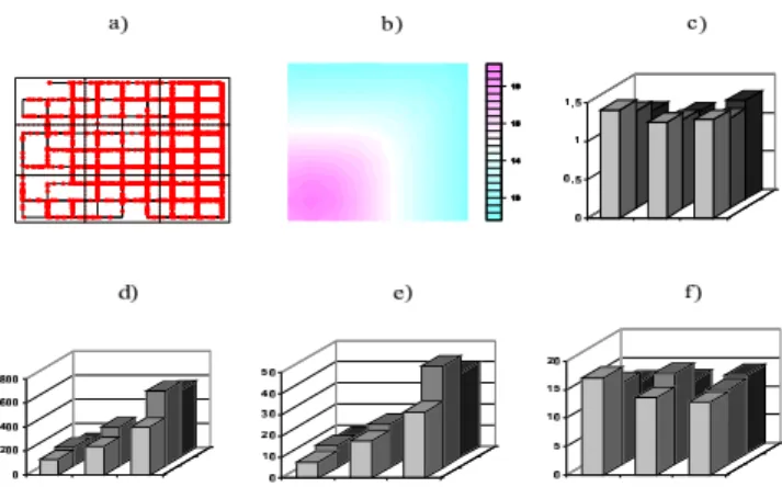
We present numerical results of the simulation for the grid size m=9. The grid A is subdivided onto boxes Ai j,i,j=1, . . . ,3, see the thick lines in Fig. 1a.

Further parameters are N=20 (number of realisations of Λ), M =1000 (number of time steps), △=0.1, n=65 in Eq. 6. We thus obtain the term (Eq. 7) equal to 0.025a. We choose a equal to 100 in the lower left box A31 and equal to 1 elsewhere to obtain an

inhomogeneous ˜Λ. Thus the n-th term in Eq. 6 has mean value 0.02636, which is small in comparison to

˜

Λvalues in Fig. 1b.

Fig. 1. 3×3 grid of boxes, a) simulated random walk with spikes, b) a simulated inhomogeneous intensity, c) Fano factors, d) histogram of the numbers of spikes, e) histogram of time units spent in a box, f) estimated expected intensity.

The data and results (estimation of Fano factor and conditional intensity) are in Fig. 1. The histograms in d) and e) are naturally of a similar shape resulting from a). The Fano factors estimated in c) are clearly above 1. Using Eq. 2 the estimated expected intensity in f) corresponds to the theoretical intensity in b). Unfortunately for further characteristics estimation, e.g., for the variance of the driving intensity, there are no simple estimators available. Therefore we proceed using the filtering techniques.

FILTERING

BACKGROUND AND DISCRETIZATION

Another rigorous approach to the problem of the inference of the driving intensity Λ and its characteristics is the filtering (Fishman and Snyder, 1976; Lechnerov´a et al., 2008). Given a realisation of a spatio-temporal point process X of spikes and given a trajectory of the path Y, the solution of the nonlinear filtering problem is the conditional expectation E[Λ|X,Y]which is not explicitly available. Here the Bayes formula for probability densities is useful

f(λ|x,y)∝ f(x|λ,y)f(λ|y),

since from the definition of the doubly stochastic Poisson process f(x|λ,y) is a density of an inhomogeneous Poisson process with intensity functionλ. We will assume in the following thatΛ,Y are stochastically independent. Then,

and the aim is to simulate a sample from the density f(λ|x) which enables to solve the filtering problem and estimate empirically any characteristics of Λ including the overdispersion. Simulation is possible using Markov chain Monte Carlo (MCMC) techniques by means of one of the following approaches: the use of a) discrete grid, b) point process densities w.r.t. unit Poisson process.

Consider a parallelepiped W⊂R3. In the approach a) we consider a spatio-temporal grid of cubes with centroids {ci jk} ⊂ W as above and denote λi jk =

Λ(ci jk). Let ni jk be the counts of spikes in each cube.

Then for the joint conditional densities it holds

f({λi jk}|{ni jk})

∝ f({ni jk} | {λi jk})f({λi jk}) ≈

∏

i jk

f(ni jk|λi jk)

∏

f({λi jk,i,j} | {λi j,k−1,i,j}).

In the right hand side of the last formula there is a product of marginal Poisson probabilities f(ni jk |

λi jk) (because of independence property of the Cox

process given intensity) and a second product of transition densities (from the Markov property in time of a spatio-temporal OU process, see Barndorff-Nielsen and Schmiegel, 2004). In this second product

{λi jk,i,j} is the set of all λi jk where i,j vary along

the index set, but k is fixed (while in{λi jk}all indexes

vary).

The use of MCMC requires a closed formula for the transition densities, which may have atoms and are hard to evaluate . The algorithm was demonstrated for a different model of spatio-temporal log-Gaussian Cox process in Brix and Diggle (2001). The approximation works well if the intensity varies slowly w.r.t. the grid step size which is not the case for the jump model (Eq. 4). Therefore we look for another method.

POINT PROCESS APPROACH TO FILTERING

Because of the jump character of the model (Eq. 4) with Poisson basis, the second approach to filtering, based on the point process of jumps of Z is available. Let W =A×[0,T], denote the data x={τj} where

each τj reflects time and location of a spike on y. In

Eq. 9, we have now

f(x|λ,y)∝exp

−

Z T

0 λ

(yt,t)d t

∏

τi∈x

λ(τi),

with the proportionality constant independent of both x andλ. It is a density (w.r.t. a unit Poisson process) of an inhomogeneous spatio-temporal Poisson process

with intensity function λ. For the driving intensity function we have from Eq. 4 a representation,

Λ(v,t) =

∑

tj≤t

etj−t ₁

B_{t j}−t(v)(ξj), (10)

where {ξj,tj}, ξj ∈ R2 locations, tj ∈ R times, are

events of the auxiliary spatio-temporal Poisson point process corresponding to the Poisson basis Z.

In comparison with Eq. 6 instead of simulating Poisson counts here we shall simulate each individual jump of Z. The region W0 where these points are

simulated is shown in Fig.2.

A

W

0 T

W0

Fig. 2. The enlarged window W0 of W, where A is the arena and [0,T] the time interval. The points

{ξj,tj} of the auxiliary process are simulated in W0. Points outside this region should have no or very little contribution to the driving intensity (Eq. 10) using similar reasoning as in Eq. 7.

The unconditional density

f(λ) = f {ξj,tj}nj=1

_∝

αn_{, n variable,}

in Eq. 9 is a density (w.r.t. unit Poisson process in W ) of the auxiliary point process {ξj,tj} of jumps

(considered homogeneous here) with intensityα>0,

which representsΛ.

The Metropolis-Hastings birth-death algorithm (Møller and Waagepetersen, 2003) can be used to simulate the MCMC chain {ξj,tj}(l), l = 0, . . . ,J,

ESTIMATION OF CONDITIONAL INTENSITY CHARACTERISTICS

Using the MCMC iterations of the auxiliary point process we evaluate the l-th iteration Λ(l)(v,t) from Eq. 10. Let 0<K <J be the burn-in of the chain, k=J−K,and let a single realisation of Y,X be given. Analogously to Eq. 1, we pay attention here to time averaged characteristics, but any quantity derived from

Λcan be obtained. For the discrete random walk with M time steps let

ˆ

Λ(l)_{(v) =} 1

M

M−1

∑

q=0

Λ(l)_(v,q△),

we get the conditional expectation of intensity estimated as,

c

EΛ(v) =1

k

J

∑

l=K+1

ˆ

Λ(l)_{(v), (11)}

and the conditional variance of intensity estimated as

d

varΛ(v) = 1

k−1

J

∑

l=K+1

ˆ

Λ(l)_{(v)−EcΛ(v)}2_{. (12)}

From N independent realisations of Y,X by evaluating corresponding N MCMC chains as above and averaging over realisations we can obtain estimates of unconditional quantities E[Λ(v,t)],var[Λ(v,t)].

NUMERICAL RESULTS AND

CONCLUSIONS

We simulated an experiment Y,X with homogeneous intensityΛ and used the point process approach to the filtering. A grid of 2×2 boxes was used with 20 time steps, m=2,△=1,α =1 and Bs(x1,x2) = [x1+_us,x1−_us]×[x2+_us,x2−s_u], s≤0,

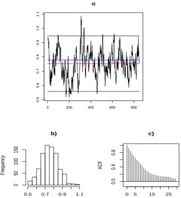
where u= 5. The MCMC chain of time averaged conditional intensity is in Fig. 3 together with its characteristics. We can observe an approximately Gaussian character in b) of the chain in a) and its slow mixing (decrease of autocorrelation function) in c). Denote Ei jthe mean in Eq. 11 andσii the standard

deviation (square root of Eq. 12). The results obtained on the grid are

Ei j=

0.746 0.758 0.768 0.714

, (13)

σi j=

0.097 0.099 0.101 0.104

. (14)

0 200 400 600 800

0.5

0.6

0.7

0.8

0.9

1.0

1.1

a)

b)

Frequency

0.5 0.7 0.9 1.1

0

50

100

150

0 5 15 25

0.0

0.4

0.8

c)

ACF

Fig. 3. 85×103iterations of MCMC chain in the first of 4 boxes, a) the conditional expectation of intensity and its b) histogram, c) autocorrelation function. The horizontal axes in a) and c) correspond to number of iterations times 100. The horizontal axis in b) and the vertical axis in a) correspond to conditional expectation of intensity values. The blue line level in a) is the time averaged realisation of Eq. 10 at the corresponding grid point, used for the simulation of data X . The red line is the resulting level E11=0.746 in Eq. 13. The bounds in a) correspond to E11±2σ11 whereσ11=0.097 is the standard deviation in Eq. 14.

In the paper we discussed the stochastic modelling and simulation of an action consisting of random events which appear in time and space, with a similarity to a neurophysiological experiment. We developed the filtering approach to the estimation of conditional characteristics of the driving intensity of the spatio-temporal Cox process model. From the two approaches to filtering the one based on discretization is analytically and algorithmically demanding, since the transition distribution is hard to evaluate. On the other hand the presented point process approach is only computationally demanding, which does not make serious problems.

ACKNOWLEDGEMENT

The research was supported by the projects MSM0021620839, IAA101120604 and GA ˇCR201/05/ H007.

REFERENCES

Barndorff-Nielsen O, Schmiegel J (2004). L´evy based tempo-spatial modelling; with applications to turbulence. Usp Mat Nauk 159:63–90.

Brix A, Diggle P (2001). Spatio-temporal prediction for log-Gaussian Cox processes. J Royal Statist Soc B 63:823– 41.

Daley DJ, Vere-Jones D (1988). An introduction to the theory of point processes. New York: Springer.

Eden UT, Frank LM, Barbieri R, Solo V, Brown EN (2004). Dynamic analyses of information encoding by neural ensembles. Neural Comput 19, 5:971–98.

Fano U (1947). Ionization yields radiations. II. The fluctuations of the number of ions. Phys Rev 72:26–9. Fenton AA, Muller RU (1998). Place cell discharge is

extremely variable during individual passes of the rat through the firing field. Proc Nat Acad Sci USA 95:3182–7.

Fishman PM, Snyder D (1976). The statistical analysis of space-time point processes. IEEE Trans Inf Theory 22:257–74.

L´ansk ´y P, Vaillant J (2000). Stochastic model of the overdispersion in the place cell discharge. Biosystems 58:27–32.

Lechnerov´a R, Helisov´a K, Beneˇs V (2008). Cox point processes driven by Ornstein-Uhlenbeck type processes. Methodol Comput Appl Probab, in print. DOI: 10.1007/s11009-007-9055-1

Møller J, Waagepetersen R (2003). Statistics and simulations of spatial point processes. Singapore: World Sci.

Prokeˇsov´a M, Hellmund G, Vedel Jensen E (2006). On spatio-temporal L´evy based Cox processes. In: Lechnerov´a R, Saxl I, Beneˇs V, eds. S4G. Proceedings of the International Conference on Spatial Statistics, Stereology, Stochastic Geometry. Praha: J ˇCMF, 112–7. Schoenberg FP, Brillinger DR, Guttorp PM (2002).