ADAPTIVE PARAMETER SELECTION FOR GRAPH-CUT BASED
SEGMENTATION ON CELL IMAGES
K
AZEEMO. O
YEBODEB
ANDJ
ULESR. T
APAMOSchool of Engineering, Howard College Campus, University of KwaZulu-Natal, Durban, 4041, South Africa e-mail: [email protected]; [email protected]
(Received May 9, 2015; revised August 14, 2015; revised November 24, 2015; accepted December 15, 2015)
ABSTRACT
Graph cut segmentation approach provides a platform for segmenting images in a globally optimised fashion. The graph cut energy function includes a parameter that adjusts its data term and smoothness term relative to each other. However, one of the key challenges in graph cut segmentation is finding a suitable parameter value that suits a given segmentation. A suitable parameter value is desirable in order to avoid image over-segmentation or under-over-segmentation. To address the problem of trial and error in manual parameter selection, we propose an intuitive and adaptive parameter selection for cell segmentation using graph cut. The greyscale image of the cell is logarithmically transformed to shrink the dynamic range of foreground pixels in order to extract the boundaries of cells. The extracted cell boundary dynamically adjusts and contextualises the parameter value of the graph cut, countering its shrink bias. Experiments suggest that the proposed model outperforms previous cell segmentation approaches.
Keywords: cell segmentation, energy function, graph cut, parameter selection.
INTRODUCTION
Cell segmentation provides an opportunity for experts in the medical sciences to diagnose medical conditions of cancer or tuberculosis with a clear perspective. This suggests that to achieve a fast and objective diagnosis, a reliable and robust segmentation framework is essential. Graph cut provides this platform leveraging a globally optimised segmentation strategy. However, one of the key challenges of graph cut is the selection of a suitable parameter value. The parameter value plays a key role in the segmentation of images by ensuring that important parts of cells such as edges are revealed after segmentation. These parts are often lost when segmenting elongated cells (Vicente et al., 2008).
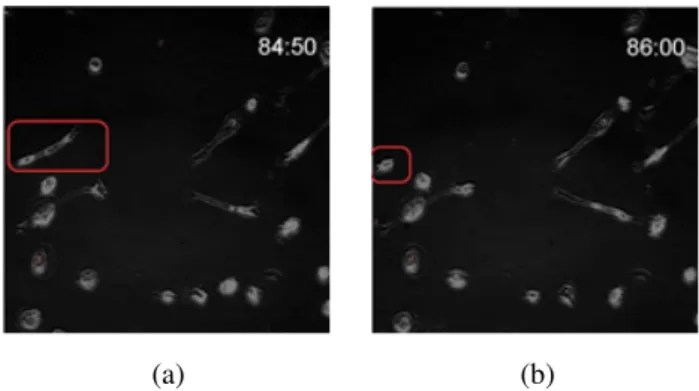
Segmentation of cell images provides a platform to monitor closely cell mobility relative to the cells’ existence and interaction with other surrounding bodies. This process provides the basis for medical diagnoses through observation of shapes and forms of segmented region. However, cells often suffer from non-uniform illumination, with blurry cell boundaries delineating them from their background. In addition, live cells possess dynamic shapes and over selected time frames, they take on different shapes like oval, elongated or irregular. This makes segmentation difficult when using techniques based on cell shapes. Consider the highlighted cell in Fig. 1a at time 84.50 and its position in Fig. 1b at time 86:00; it is clear that the shape of the cells has changed over the time interval. Accurate monitoring or tracking of these cell shapes over a given time frame is therefore crucial
for discovery of abnormalities such as cancerous cells (Bengtsson, 1999).
(a) (b)
Fig. 1. Cell images. (a) Original position of highlighted cell. (b) Final position of highlighted cell from (a).
Based on the aforementioned facts, the objective of this work is to develop a robust graph cut algorithm that regularises graph cut data term as well as its smoothness term by dynamically altering its parameter value. Several cell segmentation approaches have been proposed in literature leveraging graph cut. For example, a two-stage cell segmentation approach is proposed by Danˇek et al. (2009). The first stage segments isolated cells from their background, while the second stage deals with touching cells or cell clusters using shape priors.
Fig. 2. Illustration showing the compromise between data term and smoothness term. (a) Original image. (b) Segmentation with small parameter value, ensuring a smoothened segmentation while, however, ignoring cell details such as boundaries after segmentation. (c) Segmentation with large parameter value, retaining some cell edges after segmentation; however, image is noisy. (d) Optimal segmentation with some edges still missing.
(a) (b)
Fig. 3.(a) Ground truth. (b) Graph cut taking shorter route (red boundaries) for segmentation in place of longer route (green boundaries) as seen in (a).
Al-Kofahi et al. (2010) presented an automatic cell segmentation where an image is segmented into foreground and background using graph cut, then a second graph cut segmentation follows to delineate touching cells. Chen et al. (2008) adopted a graph cut based active contour (GCBAC) where the active contour constrains graph cut segmentation to areas of interest. Qi (2014) proposed a method for segmenting clustered cells through graph cut. The isolation of cell clusters is carried out based on the knowledge that cells are spherical in shape. In addition, a merging algorithm for object segmentation is proposed by Lin et al. (2003) where images are split into units, then a merging algorithm assembles neighbouring units together based on homogeneity criteria. The merging algorithm is explored for cell segmentation by Coelhoet al.(2009) and also for object segmentation by Roy and Biswas (2015). Lastly, a supervised cell segmentation based on cell shape and texture properties is proposed by Chenet al.(2013).
While the above approaches give good segmentation results, some of them are not robust in terms of cell over-segmentation. For example, the method proposed by Al-Kofahiet al.(2010) may not perform well when confronted with elongated cells because their approach is based on blob shape priors. Similarly, the GCBAC technique (Chen et al., 2008) may result in under-segmentation, because cells have varying intensity levels.
Our observation of the shrink bias of graph cut and the poor segmentation results of non-uniform illuminated cell images with unclear boundaries also motivates this research. We therefore propose a cell segmentation method that extracts cell boundaries and can be used to adjust dynamically the relative importance of graph cut data term to the smoothness term. The main difference between the proposed approach and the previous graph cut cell segmentation is that instead of using a static regularisaation parameter for graph cut segmentation, the proposed approach uses knowledge about extracted cell boundaries to adjust dynamically graph cut parameter value. This model ensures that cell boundaries are not reduced by graph cut during segmentation. Furthermore, the proposed model saves segmentation time since manual tuning of graph cut parameter value is unnecessary.
RELATED WORKS
for graph cut parameter selection; they developed an algorithm that selects a good segmentation based on an array of graph cut parameter values. The selection of best segmented image is based on texture and homogeneity characteristics. Peng and Veksler (2008) model uses a single parameter value throughout the whole image for segmentation. However, over-segmentation or under-over-segmentation may occur due to the fact that some portions of the image may require less smoothening than others (for example, object with blurry boundary) (Candemir and Akgul, 2010).
Furthermore, in Candemir and Akgul (2010) an adaptive parameter selection is introduced for object segmentation. In this approach, the boundary of the object of interest is carved by a canny edge detector (Canny, 1986). Then the result is used to regularise the parameter value of graph cut. However, for non-homogeneous cell images, cell boundary may not be extracted sufficiently, giving rise to over-segmentation or under-over-segmentation. Vicente et al. (2008) incorporated a connectivity prior in their graph cut algorithm. Although their algorithm improves graph cut segmentation, users are required to inscribe additional scribbles during the process. This approach is susceptible to time wasting.
Graph cut with shape prior has also been researched in literature for object segmentation (Freedman and Zhang, 2005). However, a limitation of this method is the choice of an appropriate graph cut parameter value (λ; Langet al., 2009; Wanget al., 2013).
PAPER ORGANISATION
The rest of the paper is organised as follows: related works with respect to graph cut parameter selection are reviewed, followed by the introduction of proposed model. In the next section, proposed model is evaluated on public and private datasets with discussions put forward. Future improvements on proposed model are discussed in the conclusion.
MATERIAL AND METHODS
The proposed model takes advantage of image logarithmic transform. This is necessary because of the high variability of foreground pixel values and provides a way to shrink the range of foreground pixel values. Foreground pixels having low values are compressed logarithmically and transformed into high values to enhance the distinctive categorisation of foreground pixels into boundary pixels and non-boundary pixels. This transformation is important in order to adjust and contextualise graph cut parameter value across the distinctive categorisation of foreground pixels. Invariably, weights of pixels found
in cell boundary are adjusted. An image smoothening processs begins the model.
IMAGE SMOOTHING
In order to reduce noise, cell image is smoothened using the 2D Gaussian filter defined as follows:
F(a,b) = 1
2π σ2 exp
−a 2+b2
2σ2
, (1)
whereσdetermines the smoothening degree. Given an imageI(x,y), an enhancement with the Gaussian filter F(a,b) of size m×n is obtained by performing the convolution ofF(a,b)withI(x,y)defined by Eq. 2:
IG(x,y) =
m−1
∑
a=0
n−1
∑
b=0
F(a,b)I(x−a,y−b). (2)
IG(x,y)is the smoothened version of imageI(x,y).
CELL BOUNDARY EXTRACTION
Cell images have varying degrees of intensity levels; hence they do not always have homogeneous structure (Chen et al., 2008). Furthermore, cells possess weak boundaries, which makes it difficult to identify or isolate individual cells in an image frame by visual analysis (Al-Kofahi et al., 2010). In this work, cell boundaries are revealed by shrinking the dynamic range of foreground pixel values in the image. The reason for this is to ensure that the foreground pixel values are compressed into a minimum value range. Another justification for shrinking the dynamic range of cell images is that they are of low quality and appear to fade into the background. As a result, we transform their foreground pixel values from a low pixel value to a high pixel value. Hence it is important to reveal cells at the point at which they begin to fade and blend with the background. The logarithmic function is defined in Eq. 3:
IL(x,y) =c∗IG(x,y)α, (3)
where IG(x,y) is the intensity value of pixel at the location(x,y)of the smoothened input image.IL(x,y)
indicates the intensity value of pixel at location(x,y)of the output image.α (alpha) controls the level of pixel shrinkage, andcis the scaling factor.
Algorithm 1 Cell Boundary Extraction
Require: I, . Original Image
Ensure: Ib . Extracted cell boundary image
1: Iis Guassian-filtered using Eq. 2 and result saved inIG
2: Logarithmically enhanceIGusing Eq. 3, save result inIL
3: BinariseILusing Otsu thresholding, save result inIo
4: Define a structuring elementBof ones, of size 7 by 7 5: UseBto erodeIo, save result inIErode(IErode= (Io B))
6: SubtractIErodefromIo, save result inIb(Ib=Io−IErode)
end
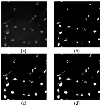
Fig. 4. Cell boundary extraction process. (a)
Smoothened images (IG). (b) Logarithmically
transformed images (IL). (c) Binarised cell images using Otsu thresholding (Io). (d) Cell boundary extraction (Ib).
GRAPH CUT ENERGY FUNCTION DERIVATION
An image is represented using a graphG= (V,E), where the graph nodesV correspond to image pixels (a,b,d,e,f,g in Fig. 5) and graph edges E are links between nodes (examples of edges in Fig. 5 are O−
a,C−a,a−b,b−d, anda−e), corresponding to links between pixels in the image context. Additionally, nodes OandCare in the setV representing terminal links. The objective is to assign a labelL∈ {0,1}to pixels in the segmented image where 0 and 1 represent background and foreground respectively. A Bayesian framework is used to model image segmentation. Let K be the segmentation of a given image whileI is the measured brightness function, then we have
P(K|I) =P(I|K)P(K)
P(I) . (4)
Suppose pixel positions in a cell image i =
0,1, . . .n, then the intensity values of these pixels which depend on K are given as I(0),I(1), . . . ,I(n), where each intensity value is independent of the other. A joint probability of their intensity values is given as
Fig. 5.Representation of an image in graph context.
P(I|K) =P(I(1)|K)P(I(2)|K). . .P(I(n)|K) =
n
∏
i=0
P(I(i)|K). (5)
In Eq. 5, P(I|K) gives the likelihood function. It emphasises the cell image creation process, that is, the probability of quantifying I(i) when K is given. In Eq. 4,P(K),P(I)are the prior probabilities; P(K) describes the partitioning of grey values of image pixels into ones and zeros whileP(I)describes their intensity distribution. The maximum a posteriori (MAP) estimation (Boykov and Jolly, 2001) for image segmentation is defined as in Eq. 6:
KMAP=arg max K
P(I|K)P(K)
P(I) . (6)
P(I) is a constant and the estimation can then be rewritten as
KMAP=arg max
K P(I|K)P(K). (7) The negative logarithm of the posterior probability can be minimised yielding Eq. 8:
E(K) =−log n
∏
i=1
P(I(i)|K)−logP(K). (8)
The negative logarithm of the probability gives the energy function E(K). Since the logarithm of a product is equal to the sum of logarithms of terms of the product, hence the energy function is rewritten in Eq. 9:
E(K) =
n
∑
i=1
−log(P(I(i)|K))−logP(K). (9)
(Greiget al., 1989; Boykov and Jolly, 2001), which is given as
B(K) =−logP(K), (10)
=
∑
(i,j)∈N exp
−|I(i)−I(j)| 2
2σ2
· 1
ed(i,j) .
In the right-hand-side of Eq. 10, N is the set of neighbouring pixels (iand j) in a given image.ed(i,j)
provides the Euclidean distance between i and j (Boykov and Jolly, 2001).B(K)favours neighbouring pixels (i and j) having similar greyscale intensities. B(K) has a low value when neighbouring pixels (i and j) have different greyscale intensities. Hence the behaviour ofB(K)suggests a cut when neighbouring pixels have different intensity values.σ describes how much we are concerned about pixel similarity. Then, Eq. 11 becomes the energy function,
E(K) =λR(K) +B(K), (11)
where
R(K) =−
n
∑
i=1
log(P(I(i)|K)).
Within the context of a graph (Fig. 5) the data termR(K)gives weight to each of the graph edges, for example, edgesO−a,C−a,O−b,O−e,O−f,O−
g,C−e,C− f and C−b in Fig. 5. The weight of these edges is determined by the negative logarithm of the probability of a pixel being a foreground or background pixel, considering sample pixels selected by user. B(K) provides weight to node edges, for example, edges a−b,b−d and a−e in Fig. 5. The energy function in Eq. 11 is similar to the graph cut energy function introduced by Boykov and Jolly (2001); the first term gives the data term while the second term gives the smoothness term. λ regulates the relative importance of the data term versus the smoothness term.
GRAPH CUTS ENERGY FUNCTION MODIFICATION
We seek to adjust the parameter value λ dynamically in the graph cut energy function. This dynamic adjustment is motivated by Ib as discussed earlier. Ib increases the weights of pixels at cell boundaries in order to survive a cut. Thus, the graph cut energy function may be rewritten as follows:
E(K) =λˆ R(K) +B(K). (12)
where ˆλ =λ(βIb+Inb), Ibis boundary pixel, and Inb is non-boundary pixel.
In Eq. 12,β(β =2,3,4, . . .)defines the weighting factor around cell boundaries. Eq. 12 shows that the weights on cell boundary pixels via the data term are increased. This development makes the parameter value adaptive. Putting the boundary pixel weights above other foreground pixel weights gives an assurance that cell boundaries can survive the graph cut shrink bias. The Max-Flow Min-Cut algorithm proposed by Boykov and Kolmogorov (2004) has been used for segmentation. Algorithm 2 summarises the cell segmentation process.
Algorithm 2 Segmentation of cell image using logarithmic transform and graph cut
Require: I, . Greyscale image Ensure: IS . Segmented image
1: Iis Gaussian-filtered using Eq. 2 and the result is saved in
IG
2: FindIbforIusing Algorithm 1
3: Construct the graphGfromIG
4: foreach pixel (x,y) ofIGfor the data termdo
5: ifIG(x,y) ==Ib(x,y)then
6: Ib=1,Inb=0, ˆλ=β λ
7: AddweightλˆR(K)toIG(x,y)inGto form a weight
link with terminal nodeO
8: Addweight0 toIG(x,y)inGto form a weight link
with terminal nodeC
9: else
10: Ib=0,Inb=1, ˆλ=λ
11: AddweightλˆR(K)toIG(x,y)inGto form weight
links with terminal nodesOandC
12: end if
13: end for
14: foreach pixel(x,y)ofIGfor smoothness termdo
15: Add weightB(K)to the link that connects(x,y)to its adjacent neighbours
16: end for
17: Store the Minimum Cut Maximum flow ofGinIS
end
RESULTS
DATASET
are manually constructed. In order to strengthen the evaluation process further, public available dataset U2OS (Coelho et al., 2009) containing 48 images was also used to test the performance of the proposed model. Each image has an average of 40 cells.
EVALUATION
The performance of the proposed model is measured using the Rand Index (RI), Hausdorff distance (H) and Sensitivity (ST) metrics (Coelho et al., 2009). High values ofRIandST and a low value of H are indicative of good segmentation. The Rand Index (RI) is defined in Eq. 13:
RI(%) = (TP+TN)
(TP+TN+FP+FN) , (13)
where true positive (TP) defines the total number of foreground pixels in the segmented image S (binary) that overlap foreground pixels in the ground truth G (binary). True negative (TN) gives the total number of background pixels in the segmented image S that overlap background pixels in the ground truthG. False positive (FP) defines the total number of foreground pixels in the segmented image S that are referenced as background pixels in the ground truth G. False negative (FN) defines the total number of background pixels in the segmented image S that are referenced as foreground pixels in the ground truthG. Hausdorff distance (H) is defined in Eq. 14 as
H(G,S) =max{V(l):Sl6=Gl}, (14) wherel indicate co-ordinates of considered pixel pair in S and G. V(l) gives the distance between the considered pixel pair inSandG. The sensitivity (ST) formula is obtained by:
ST(%) = TP
TP+FN . (15)
PARAMETER SELECTION
In this experiment, the weight factorβ as well as λ, the graph cut parameter, are both set to 20. For optimal image enhancement (Eq. 3), the value of c is set to two. This value is used for both public and private dataset. However, α is set to 0.45 for public dataset and 0.50 for the private dataset. For parameters with respect to Gaussian smoothening indicated in
Eq. 2, we reflect on all potential combinations ofσand the Gaussian kernel size m×n {σ,m,n}={2,3,3},
{2,5,5}, {2,10,10}, {3,3,3}, {3,5,5}, {3,5,5} and
{2,10,10}. The parameter{2,10,10}minimises noise better than other combinations, hence it is adopted for proposed model.
RESULTS DESCRIPTION
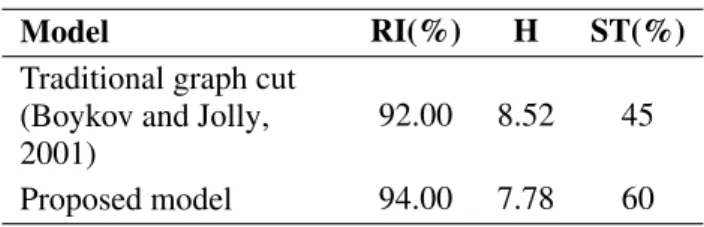
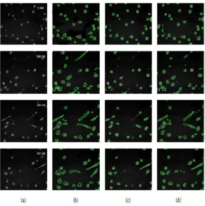
Some results of the application of proposed model on cell images are presented. The proposed model shows improved performance over other models while considering metricsH,ST andRI as seen in Tables 1 and 2 and Figs. 6 and 7. These results (Fig. 6 and Table 1) demonstrate that elongated cells are segmented to a reasonable degree. However, in extreme cases, where cell boundaries are not visible, poor results are obtained. Table 1 also indicates that the shrink bias of graph cut is reasonably minimised by proposed model; this is evident in the metrics ST and RI. In these metrics, the contribution ofFNis reduced as compared to the traditional graph cut.
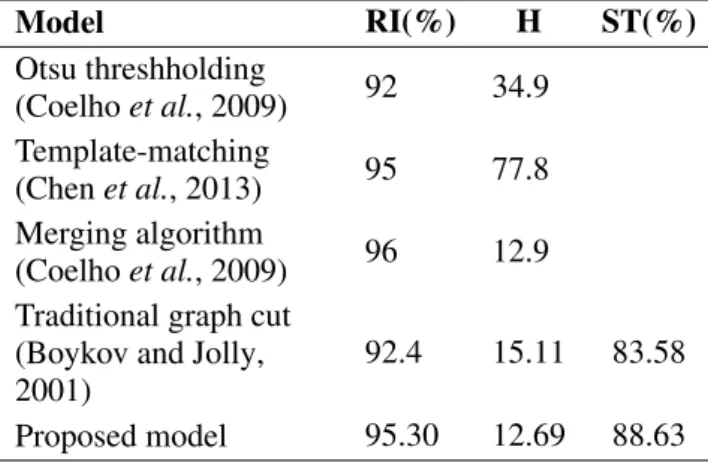
This analysis (shrink bias) also holds for the public dataset as seen in Table 2, in terms of metricsH and RI; proposed model performs better as compared to other cell segmentation models. However, in terms of the RI, proposed model is the second best. This can be attributed to the fact that some extracted boundaries via Algorithm 1 may not be actual cell boundaries, but noise. Since boundaries of noise may have been extracted, the FP component in the RI metric is invariably increased. This obviously degrades the performance of the proposed model. This shows that a more sophisticated filtering method should be adopted in order to reduce noise significantly. The merging algorithm (Table 2) performs better with respect to minimising its FP component of the RI metric. The template-matching algorithm also shows good performance with respect toRI; however, its H value is the highest.
Table 1. RI, H and ST evaluation of proposed model and traditional graph cut on private dataset.
Model RI(%) H ST(%)
Traditional graph cut (Boykov and Jolly, 2001)
92.00 8.52 45
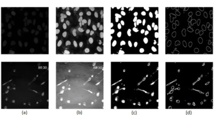
Fig. 6. Visual results of segmentation of four samples of cell images from private dataset. (a) Original images. (b) Ground truth. (c) Traditional graph cut. (d) Proposed model.
Table 2. RI, H and ST evaluation of proposed model and traditional graph cut on public dataset.
Model RI(%) H ST(%)
Otsu threshholding
(Coelhoet al., 2009) 92 34.9 Template-matching
(Chenet al., 2013) 95 77.8 Merging algorithm
(Coelhoet al., 2009) 96 12.9 Traditional graph cut
(Boykov and Jolly, 2001)
92.4 15.11 83.58
Proposed model 95.30 12.69 88.63
DISCUSSION
One contributing factor to the improved performance of proposed model is the incorporation of cell boundary into graph cut. By giving more weight to pixels at cell boundaries, the shrink bias of graph cut is mitigated. The contributing factor to the poor performance of traditional graph cut which is obvious in Fig. 6 is the inability to adjust its parameter (λ) value adaptively; hence the shrink bias of graph cut comes into play.
However, when images contain touching cells or dense cells, there is a reduction in the performance of the model. For example, the model cannot draw boundary lines to separate touching cells. The model sees touching cells as a single cell. For future work, one may investigate the possibility of incorporating the segmentation of cell clusters. Our approach is an interactive cell segmentation process where user selects sample foreground and background pixels. The automation of foreground and background sample pixel selection may further improve the performance of proposed model. In addition, a more robust approach that is immune to noise for boundary extraction is suggested for better performance.
CONCLUSION
This work has explored adaptive graph cut parameter selection. This is achieved by cell boundary extraction and fusing this into the graph cut parameter value, thereby providing an avenue to alter dynamically pixel weights in the graph formulation. This development reasonably counters the shrink bias of graph cut. The proposed model has been tested on 78 cell images with an average running time of 19
seconds per image on a Windows 7, Core i5 processor, and experiment results indicate a better segmented output. This model provides a basis for objective diagnosis of diseases such as tuberculosis or cancer by medical experts.
ACKNOWLEDGMENT
The authors would like to thank Dr Alex Sigal of the KwaZulu-Natal Research Institute for Tuberculosis and HIV (K-RITH), for providing the private dataset used in this research.
REFERENCES
Al-Kofahi Y, Lassoued W, Lee W, Roysam B (2010). Improved automatic detection and segmentation of cell nuclei in histopathology images. IEEE T Bio Med Eng 57:841–52.
Bengtsson E (1999). Fifty years of attempts to automate screening for cervical cancer. Med Imaging Technol 17:203–10.
Boykov Y, Jolly MP (2001). Interactive graph cuts for optimal boundary and region segmentation of objects in n-d images. In: Proc 8th IEEE Int Conf Comput Vision (ICCV 2001) 1:105–12.
Boykov Y, Kolmogorov V (2004). An experimental comparison of min-cut/max- flow algorithms for energy minimization in vision. IEEE T Pattern Anal 26:1124– 37.
Candemir S, Akgul YS (2010). Adaptive regularization parameter for graph cut segmentation. In: Campilho A, Kamel M, eds. Proc 7th Int Conf Image Anal Recogn (ICIAR). Lect Not Comput Sci 6111:117–26.
Canny J (1986). A computational approach to edge detection. IEEE T Pattern Anal 8:679–98.
Chen C, Li H, Zhou X, Wong ST (2008). Constraint factor graph cut-based active contour method for automated cellular image segmentation in rnai screening. J Microsc 230:177–91.
Chen C, Wang E, Ozolek J, Rohde GK (2013). A flexible and robust approach for segmenting cell nuclei from 2d microscopy images using supervised learning and template matching. Cytometry A 83:495–507.
Coelho LP, Shariff A, Murphy R (2009). Nuclear segmentation in microscope cell images: A hand-segmented dataset and comparison of algorithms. In: Proc IEEE Int Symp Biomed Imaging (ISBI ’09) 518– 21.
Freedman D, Zhang T (2005). Interactive graph cut based segmentation with shape priors. In: Proc IEEE Int Conf Comput Vision Pattern Recogn (CVPR 2005) 755–62. Greig D, Porteous B, Seheult A (1989). Exact maximum a
posteriori estimation for binary images. J R Stat Soc B Met 51:271–9.
Lang X, Zhu F, Hao Y, Wu Q (2009). Automatic image segmentation incorporating shape priors via graph cuts. In: Proc Int Conf Inform Autom (ICIA ’09) 192–5. Lin X, Adiga U, Olson K, Guzowski J, Barnes C,
Roysam B (2003). A hybrid 3d watershed algorithm incorporating gradient cues and object models for automatic segmentation of nuclei in confocal image stacks. Cytometry A 56A:23–36.
Peng B, Veksler O (2008). Parameter selection for graph cut based image segmentation. In: Everingham M,
Needham C, eds. Proc Brit Mach Vision Conf (BMVC). 16.1–10
Qi J (2014). Dense nuclei segmentation based on graph cut and convexity concavity analysis. J Microsc 253:42–53. Roy P, Biswas P (2015). A parallel legion algorithm and cell-based architecture for real time split and merge video segmentation. J Real Time Image Process (in press).
Vicente S, Kolmogorov V, Rother C (2008). Graph cut based image segmentation with connectivity priors. In: Proc IEEE Int Conf Comput Vision Pattern Recogn (CVPR 2008) 1–8.