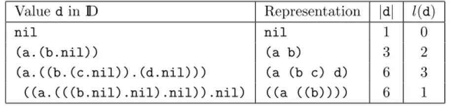
Complexity Issues in VLSI: Optimal Layouts for the Shuffle-Exchange Graph and Other Networks, Frank Thomson Leighton, 1983
Equational Logic as a Programming Language, Michael J. O’Donnell, 1985 General Theory of Deductive Systems and Its Applications, S. Yu Maslov, 1987
Resource Allocation Problems: Algorithmic Approaches, Toshihide Ibaraki and Naoki Katoh, 1988
Algebraic Theory of Processes, Matthew Hennessy, 1988
PX: A Computational Logic, Susumu Hayashi and Hiroshi Nakano, 1989
The Stable Marriage Problem: Structure and Algorithms, Dan Gusfield and Robert Irving, 1989
Realistic Compiler Generation, Peter Lee, 1989
Single-Layer Wire Routing and Compaction, F. Miller Maley, 1990 Basic Category Theory for Computer Scientists, Benjamin C. Pierce, 1991
Categories, Types, and Structures: An Introduction to Category Theory for the Working Computer Scientist, Andrea Asperti and Giuseppe Longo, 1991
Semantics of Programming Languages: Structures and Techniques, Carl A. Gunter, 1992 The Formal Semantics of Programming Languages: An Introduction, Glynn Winskel, 1993 Hilbert’s Tenth Problem, Yuri V. Matiyasevich, 1993
Exploring Interior-Point Linear Programming: Algorithms and Software, Ami Arbel, 1993 Theoretical Aspects of Object-Oriented Programming: Types, Semantics, and Language Design, edited by Carl A. Gunter and John C. Mitchell, 1994
From Logic to Logic Programming, Kees Doets, 1994
The Structure of Typed Programming Languages, David A. Schmidt, 1994 Logic and Information Flow, edited by Jan van Eijck and Albert Visser, 1994 Circuit Complexity and Neural Networks, Ian Parberry, 1994
Control Flow Semantics, Jaco de Bakker and Erik de Vink, 1996
Algebraic Semantics of Imperative Programs, Joseph A. Goguen and Grant Malcolm, 1996 Algorithmic Number Theory, Volume I: Efficient Algorithms, Eric Bach and Jeffrey Shallit, 1996
Foundations for Programming Languages, John C. Mitchell, 1996
Neil D. Jones
The MIT Press
All rights reserved. No part of this book may be reproduced in any form by any electronic or mechanical means (including photocopying, recording, or information storage or retrieval) without permission in writing from the publisher.
This book was set in Palatino by the author and was printed and bound in the United States of America.
Library of Congress, Cataloging-in-Publication Data
Jones, Neil D.
Computability and complexity: from a programming perspective / Neil D. Jones.
p. cm. -- (Foundations of computing)
Includes bibliographical references and index. ISBN 0-262-10064-9 (alk. paper)
1. Electronic digital computers -- programming. 2. Computational complexity.
I. Title. II. Series. QA76.6.J6658 1997
005.1301--dc21 96-44043
Series Foreword
vii
Preface
ix
I
Toward the Theory
1
1 Introduction 3
2 The WHILE Language 29
3 Programs as Data Objects 47
II
Introduction to Computability
65
4 Self-interpretation: Universal Programs for WHILE and I 67
5 Elements of Computability Theory 73
6 Metaprogramming, Self-application, and Compiler Generation 87
7 Other Sequential Models of Computation 111
8 Robustness of Computability 127
9 Computability by Functional Languages (partly by T. Æ. Mogensen) 137
10 Some Natural Unsolvable Problems 153
III
Other Aspects of Computability Theory
167
11 Hilbert’s Tenth Problem (by M. H. Sørensen) 169 12 Inference Systems and G¨odel’s Incompleteness Theorem 189
13 Computability Theory Based on Numbers 207
14 More Abstract Approaches to Computability 215
IV
Introduction to Complexity
237
15 Overview of Complexity Theory 239
16 Measuring Time Usage 249
17 Time Usage of Tree-manipulating Programs 261
18 Robustness of Time-bounded Computation 271
19 Linear and Other Time Hierarchies for WHILE Programs 287 20 The Existence of Optimal Algorithms (by A. M. Ben-Amram) 299
21 Space-bounded Computations 317
22 Nondeterministic Computations 335
23 A Structure for Classifying the Complexity of Various Problems 339 24 Characterizations of logspace and ptime byGOTO Programs 353
V
Complete Problems
367
25 Completeness and Reduction of One Problem to Another 369
26 Complete Problems for ptime 387
27 Complete Problems for nptime 401
28 Complete Problems for pspace 409
VI
Appendix
419
A Mathematical Terminology and Concepts 421
Bibliography 449
Theoretical computer science has now undergone several decades of development. The “classical” topics of automata theory, formal languages, and computational complexity have become firmly established, and their importance to other theoretical work and to practice is widely recognized. Stimulated by technological advances, theoreticians have been rapidly expanding the areas under study, and the time delay between theoreti-cal progress and its practitheoreti-cal impact has been decreasing dramatitheoreti-cally. Much publicity has been given recently to breakthroughs in cryptography and linear programming, and steady progress is being made on programming language semantics, computational ge-ometry, and efficient data structures. Newer, more speculative, areas of study include relational databases, VLSI theory, and parallel and distributed computation. As this list of topics continues expanding, it is becoming more and more difficult to stay abreast of the progress that is being made and increasingly important that the most significant work be distilled and communicated in a manner that will facilitate further research and application of this work. By publishing comprehensive books and specialized monographs on the theoretical aspects of computer science, the series on Foundations of Computing provides a forum in which important research topics can be presented in their entirety and placed in perspective for researchers, students, and practitioners alike.
This book is a general introduction to computability and complexity theory. It should be of interest to beginning programming language researchers who are interested in com-putability and complexity theory, or vice versa.
The view from Olympus
Unlike most fields within computer science, computability and complexity theory deals with analysis as much as with synthesis and with some concepts of an apparently ab-solute nature. Work in logic and recursive function theory spanning nearly the whole century has quite precisely delineated the concepts and nature of effective procedures, and decidable and semi-decidable problems, and has established them to be essentially invariant with respect to the computational device or logical theory used.
Surprisingly, a few similarly invariant concepts have also arisen with respect to com-putations within bounded resources: polynomial time (as a function of a decision prob-lem’s input size), polynomial storage, computation with or without nondeterminism: the ability to “guess,” and computation with “read-only” data access.
Computability and complexity theory is, and should be, of central concern for practi-tioners as well as theorists. For example, “lower complexity bounds” play a role analogous to channel capacity in engineering: No matter how clever a coding (in either sense of the word) is used, the bound cannot be overcome.
Unfortunately, the field is well-known for impenetrable fundamental definitions, proofs of theorems, and even statements of theorems and definitions of problems. In my opinion this owes to some extent to the history of the field, and that a shift away from the Turing machine- and G¨odel number-oriented classical approaches toward a greater use of concepts familiar from programming languages will render classical computability and complexity results more accessible to the average computer scientist, and can make its very strong theorems more visible and applicable to practical problems.
This book covers classical models of computation and central results in computability and complexity theory. However, it differs from traditional texts in two respects:
tech-niques and motivated by programming language theory.1
2. It relieves some tensions long felt between certain results in complexity theory and daily programming practice. A better fit is achieved by using a novel model of computation, differing from traditional ones in certain crucial respects.
Further, many of the sometimes baroque constructions of the classical theory become markedly simpler in a programming context, and sometimes even lead to stronger theo-rems. A side effect is that many constructions that are normally only sketched in a loose way can be done more precisely and convincingly.
The perspective of the book
For those already familiar with computability and complexity theory, the two points above can be somewhat elaborated.
As for the first point, I introduce a simple imperative programming language called WHILE, in essence a small subset of Pascal or LISP. The WHILE language seems to have just the right mix of expressive power and simplicity. Expressive poweris important when dealing with programs as data objects. The data structures of WHILE are particularly well suited to this, since they avoid the need for nearly all the technically messy tasks of assigningG¨odel numbersto encode program texts and fragments (used in most if not all earlier texts), and of devising code to build and decompose G¨odel numbers. Simplicityis also essential to prove theorems about programs and their behavior. This rules out the use of larger, more powerful languages, since proofs about them would be too complex to be easily understood.
More generally, I maintain that each of the fields of computability and complexity theory, and programming languages and semantics has much to offer the other. In the one direction, computability and complexity theory has a breadth, depth, and generality not often seen in programming languages, and a tradition for posing precisely defined and widely knownopen problemsof community-wide interest. Also, questions concerning theintrinsicimpossibility or infeasibility of programs solving certain problems regarding programs should be of interest to programming language researchers. For instance, many problems that turn up in the field of analysis and transformation of programs turn out to be undecidable or of intractably high complexity.
1Dana Scott was an early proponent of programming approach to automata [161], but it has not yet
In the other direction, the programming language community has a firm grasp of algorithm design, presentation and implementation, and several well-developed frame-works for making precise semantic concepts over a wide range of programming language concepts, e.g., functional, logic, and imperative programming, control operators, com-munication and concurrency, and object-orientation. Moreover programming languages constitute computation models some of which are more realistic in certain crucial aspects than traditional models.
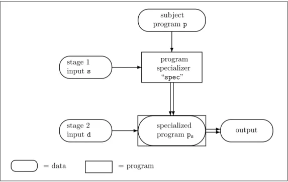
A concrete connection between computability and programming languages: the dry-as-dust “s-m-n theorem” has been known in computability since the 1930s, but seemed only a technical curiosity useful in certain proofs. Nonetheless, and to the surprise of many people, the s-m-n theorem has proven its worth under the aliaspartial evaluationor
program specializationin practice over the past 20 years: when implemented efficiently, it can be used for realistic compiling, and when self-applied it can be used to generate program generatorsas well.
Another cornerstone of computability, the “universal machine,” is nothing but a self-interpreter, well-known in programming languages. Further, the “simulations” seen in introductory computability and complexity texts are mostly achieved by informal com-pilers or, sometimes, interpreters.
As for the second point above, a tension has long been felt between computability and complexity theory on the one hand, and “real computing” on the other. This is at least in part bacause one of the first results proven in complexity is theTuring machine speedup theorem, which asserts a counterintuitive (but true) fact: that any Turing ma-chine program running in superlinear time can be replaced by another running twice as fast in the limit.2 The existence of efficient self-interpreters in programming language theory leads to the opposite result: a hierarchy theorem showing, for a more realistic computing model than the Turing machine, thatconstant time factors do matter. More precisely, given time bound f(n), where n measures the size of a problem input, there are problems solvable in time (1 +ε)f(n) which cannot be solved in time f(n). Thus multiplying the available computing time by a constant properly increases the class of problems that can be solved.
This and other examples using programming language concepts lead (at least for computer scientists) to more understandable statements of theorems and proofs in com-putability and complexity, and to stronger results. Further new results include “intrinsic” characterizations of the well-known problem classeslogspace and ptimeon the basis
2The tension arises because the “trick” used for the Turing machine construction turns out to be
of program syntax alone, without any externally imposed space or time bounds. Finally, a number of old computability and complexity questions take on new life and natural new questions arise. An important class of new questions (not yet fully resolved) is: what is the effect of theprogramming styles we employ, i.e., functional style, imperative style, etc., on theefficiency of the programs we write?
How to read this book
If used as an introduction to computability (recursive function) theory, parts I–III are relevant. If used as an introduction to complexity theory, the relevant parts are I, IV, and V, and chapters 6 through 8. The book contains approximately two semesters’ worth of material which one can “mix and match” to form several courses, for instance:
Introduction to computability (1 semester): chapters 1 through 8, chapter 10, per-haps just skimming chapter 6; and as much of chapters 9, and 11 through 14, as time and interest allow.
Introduction to complexity (1 semester): Quickly through chapters 1, 2, 3, 4, 7, 8; then chapters 15 through 19, chapters 21 through 23, and 25 through 27; and as much of the remainder as time and interest allow.
Computability and complexity (2 semesters): the whole book.
Exercises. Numerous exercises are included, some theoretical and some more oriented toward programming. An asterisk*marks ones that are either difficult or long (or both).
Correction of errors and misprints. Reports of errors and misprints may be sent to the author by e-mail, at [email protected]. A current list may be found at Worldwide Web URLhttp://www.diku.dk/users/neil/.
Goals, and chapters that can be touched lightly on first reading. The book’s overall computability goals are first: to argue that the class of all computably solvable prob-lems is well-defined and independent of the computing devices used to define it, and sec-ond: carefully to explore the boundary zone between computability and uncomputability. Its complexity goals are analogous, given naturally defined classes of problems solvable within time or memory resource bounds.
TheChurch-Turing thesisstates that all natural computation models are of equivalent power. Powerful evidence for it is the fact that any two among a substantial class of computation models can simulate each other. Unfortunately, proving this fact is unavoidably complex since the various computation models must be precisely defined, and constructions must be given to show how an arbitrary program in one model can be simulated by programs in each of the other models.
Chapters 7 and 8 do just this: they argue for the Church-Turing thesis without considering the time or memory required to do the simulations. Chapters 16, 17 and 18 go farther, showing that polynomial time-bounded or space-bounded computability are similarly robust concepts.
Once the Church-Turing thesis has been convincingly demonstrated, a more casual attitude is quite often taken: algorithms are just sketched, using whichever model is most convenient for the task at hand. The reader may wish to anticipate this, and at first encounter may choose only to skim chapters 7, 8, 16, 17 and 18.
Prerequisites
The reader is expected to be at the beginning graduate level having studied some theory, or a student at the senior undergraduate level with good mathematical maturity. Specif-ically, the book uses sets, functions, graphs, induction, and recursive definitions freely. These concepts are all explained in an appendix, but the appendix may be too terse to serve as a first introduction to these notions. Familiarity with some programming language is a necessity; just which language is much less relevant.
Novel aspects, in a nutshell
sets; Kleene’s s-m-n, second recursion, and normal form theorems; recursion by fixpoints; Rogers’ isomorphism theorem; and G¨odel’s incompleteness theorem.
Classical complexity results include study of the hierarchy of classes of problems: logspace, nlogspace, ptime, nptime, pspace; the robustness of ptime, pspaceand logspace; complete problems for all these classes except the smallest; the speedup and gap theorems from Blum’s machine-independent complexity theory.
In contrast with traditional textbooks on computability and complexity, this treat-ment also features:
1. A language of WHILE programs with LISP-like data. Advantages: programming convenience and readability in constructions involving programs as data; and free-dom from storage management problems.
2. Stronger connections with familiar computer science concepts: compilation (sim-ulation), interpretation (universal programs), program specialization (the s-m-n theorem), existence or nonexistence of optimal programs.
3. Relation of self-application to compiler bootstrapping.
4. Program specialization in the form of partial evaluation to speed programs up, or to compile and to generate compilers by specialising interpreters.
5. Speedups from self-application of program specializers.
6. Simpler constructions for “robustness” of fundamental concepts, also including functional languages and the lambda calculus.
7. A construction to prove Kleene’s second recursion theorem that gives more efficient programs than those yielded by the classical proof.
8. Proof that “constant time factorsdomatter” for a computation model more realistic than the Turing machine, by an unusually simple and understandable diagonaliza-tion proof.
9. A new and much more comprehensible proof of Levin’s important result on the existence of optimal algorithms;
10. Intrinsic characterizations of the problem classeslogspaceandptimeby restricted WHILE programs.
11. The use of programs manipulating boolean values to characterize “complete” or hardest problems for the complexity classes mentioned above.
What is not considered
There are numerous things in the enormous realm of complexity and computability theory that I have chosen not to include at all in the present text. A list of some of the most obvious omissions:
• Parallelism. In the present text all computation models aresequentialin the sense that only one operation can be executed at a time. Many models of parallel com-putation have been suggested in the literature; overviews by Karp and Valiant may be found in [96, 171].
• Approximate solutions. Another approach to solving problems whose algorithms have prohibitively long running times, is to devise a quicker algorithm which does not always give the correct answer, but only an approximate solution. Examples include numerous algorithms testing properties of graphs, e.g. by Johnson and Kann [73, 94].
• Stochastic algorithms. Some problems seem only to be solvable by programs that have prohibitively long running times. In some cases, it is possible to derive an algorithm using random numbers which runs faster, but which only returns a cor-rect result with a certain probability more than 0.5, but less than 1. Often the probability of correctness can be increased to 1−ε for any 1> ε >0 by repeat-edly running the program. Such algorithms are called stochasticor probabilistic. Examples include testing whether a given number is a prime, e.g., by Rabin [148].
• Nonuniform complexity, circuits, cell probe models. Lower bounds on computation time or space are often extremely difficult to obtain. Sometimes these can be obtained more easily by abstracting away from the algorithm altogether, and just concentrating on a problem’s combinatorial aspects. In terms of computational models, this amounts to allowing different computational methods (e.g. different circuits) for different sizes of inputs. Progress has been made in this direction, e.g., by H˚astad [66] and by Miltersen [130].
• Computing with real numbers. In the present text all computation models are concerned with countable data structures, but models of computation with real
numbers also exist, e.g., by Blum, Shub and Smale [13].
Acknowledgments
Many have helped with the preparation of the manuscript. Three in particular have made outstanding contributions to its content, style, and editorial and pedagogical matters: Morten Heine Sørensen, Amir Ben-Amram, and Arne John Glenstrup, and Jens Peter Secher and Jakob Grue Simonsen gave invaluable Latex assistance. DIKU (the Computer Science Department at the University of Copenhagen) helped significantly with many practical matters involving secretarial help, computing, and printing facilities. The idea of using list structures with only one atom is due to Klaus Grue [57].
This book is aboutcomputability theory andcomplexity theory. In this first chapter we try to convey what the scope and techniques of computability and complexity theory are. We are deliberately informal in this chapter; in some cases we will even introduce a definition or a proposition which is not rigorous, relying on certain intuitive notions.
The symbol “3” will be used to mark these definitions or propositions. All such definitions and propositions will be reintroduced in a rigorous manner in the subsequent chapters before they occur in any development.
Section 1.1 explains the scope and goals of computability theory. Sections 1.2–1.3 concern questions that arise in that connection, and Section 1.4 gives examples of tech-niques and results of computability theory. Section 1.5 describes the scope and goals of complexity theory. Section 1.6 reviews the historical origins of the two research fields. Section 1.6 contains exercises; in general the reader is encouraged to try all the exercises. Section 1.6 gives more references to background material.
A small synopsis like this appears in the beginning of every chapter, but from now on we will not mention the two sections containing exercises and references.
1.1
The scope and goals of computability theory
Computability theory asks questions such as: do there existproblemsunsolvable by any
effective procedure — unsolvable by any program in any conceivable programming lan-guage on any computer?
Our programming intuitions may indicate anoanswer, based on the experience that once a problem is made precise in the form of a specification, it is a more or less routine task to write a program to satisfy the specification. Indeed, a related intuition predomi-nated the work of Hilbert on the foundations of mathematics, as explained in section 1.6: they conjectured that all of mathematics could be axiomatized. However, we shall see that both of these intuitions are disastrously wrong. There are certain problems that cannot be solved by effective procedures.
different formalizations might lead to different theories of computability. However, one of the great insights of computability theory was the gradual realization in the 1930’s that any reasonable choice of formalization of the notion of effective procedure leads, in a certain sense, to the same theory. This has been called theChurch-Turing thesis, since Alonzo Church and Alan M. Turing first formulated and substantiated versions of this insight. Explaining why different formalizations lead to the same theory is itself one of the topics of computability theory; we thus devote considerable effort to the matter.
Granted precise definitions of the notions of problem and effective procedure, com-putability theory is concerned with the boundary between comcom-putability and uncom-putability, and addresses questions such as:
• Can every precisely stated problem be solved by some effective procedure?
• What is the class of problems that can be solved by effective procedures and its basic properties?
• What is the relationship between various problems that cannot be solved by effec-tive procedures?
If a problem can be solved by an effective procedure we shall say that is effectively solvable, or sometimes justsolvable. The result that a certain computational problem is
unsolvableis not a purely negative fact; for instance, it conveys the important knowledge that searching for an effective procedure to solve the problem is futile. This may indicate that one should try to find an approximate, solvable, solution to the problem at hand instead of trying to solve the exact, but unsolvable, problem.
In the next two sections we discuss formalization of the notions of effective proce-dure and problem. After this, we present, informally, some of the elementary results of computability theory, including two precisely stated problems which are unsolvable.
1.2
What is an effective procedure?
There are various strategies one can employ in formalizing the notion of effective proce-dure. Of course, we are free to define notions as we please, but the definitions should capture the intuitive notion of effective procedure; for example, it should not be the case that some problem is unsolvable according to our theory, but nevertheless can be solved on a real-world computer.
1.2.1
Alan Turing’s analysis of computation
Alan Turing’s analysis attempting to formalize the class of all effective procedures was carried out in 1936 [170], resulting in the notion of aTuring machine. Its importance is that it was the first really general analysis to understand how it is that computation takes place, and that it led to a convincing and widely accepted abstraction of the concept of effective procedure.
It is worth noting that Turing’s analysis was done before any computers more powerful than desk calculators had been invented. His insights led, more or less directly, to John von Neumann’s invention in the 1940’s of the stored program digital computer, a machine with essentially the same underlying architecture as today’s computers.
We give the floor to Turing. Note that by a “computer” Turing means a human who is solving a computational problem in a mechanical way, not a machine.
Computing is normally done by writing certain symbols on paper. We may suppose this paper is divided into squares like a child’s arithemetic book. In elementary arithmetic the two-dimensional character of the paper is sometimes used. But such a use is always avoidable, and I think that it will be agreed that the two-dimen-sional character of paper is no essential of computation. I assume then that the computation is carried out on one-dimensional paper, i.e., on a tape divided into squares. I shall also suppose that the number of symbols which may be printed is finite. If we were to allow an infinity of symbols, then there would be symbols differing to an arbitrarily small extent1. The effect of this restriction of the number of symbols is not very serious. It is always possible to use sequences of symbols in the place of single symbols. Thus an Arabic numeral such as 17 or 999999999999999 is normally treated as a single symbol. Similarly in any European language words are treated as single symbols (Chinese, however, attempts to have an enumerable infinity of symbols). The differences from our point of view between the single and compound symbols is that the compound symbols, if they are too lengthy, cannot be observed at one glance. This is in accordance with experience. We cannot tell at a glance whether 9999999999999999 and 999999999999999 are the same. The behaviour of the computer at any moment is determined by the symbols which
1If we regard a symbol as literally printed on a square we may suppose that the square is 0≤x≤
the paper was very long, we might reach Theorem 157767733443477; then, further on in the paper, we might find “... hence (applying Theorem 157767733443477) we have ...” In order to make sure which was the relevant theorem we should have to compare the two numbers figure by figure, possible ticking the figures off in pencil to make sure of their not being counted twice. If in spite of this it is still thought that there are other “immediately recognizable” squares, it does not upset my con-tention so long as these squares can be found by some process of which my type of machine is capable.
The simple operations must therefore include:
(a) Changes of the symbol on one of the observed squares.
(b) Changes of one of the squares observed to another square withinLsquares of one of the previously observed squares.
It may be that some of these changes necessarily involve a change of state of mind. The most general single operation must therefore be taken to be one of the following: (A) A possible change (a) of symbol together with a possible change of state of
mind.
(B) A possible change (b) of observed squares, together with a possible change of state of mind.
The operation actually performed is determined, as has been suggested [above] by the state of mind of the computer and the observed symbols. In particular, they determine the state of mind of the computer after the operation.
1.2.2
The Church-Turing thesis
The machines mentioned in Turing’s analysis are called Turing machines. The wide-ranging identification of the intuitive notion of effective procedure with the mathematical concept of Turing machine (and related identifications) has become well-known as the
Church-Turing thesis, named after Church and Turing, two pioneers of computability [170, 22, 23].
The thesis is not amenable to mathematical proof since it identifies an intuitive no-tion with a mathematical concept; however we shall provide various kinds of evidence supporting it. In one direction this is easy: the Turing machine (as well as other computa-tional models we will introduce) is sufficiently simple that its computations are certainly effective in any reasonable sense. In the other direction, Turing’s analysis is a rather convincing argument for the Turing machine’s generality.
There are many other notions of effective procedure than Turing machines, e.g.,
• Recursive functions as defined by Kleene [98]
• Thelambda calculus approach to function definitions due to Church [22, 23].
• Random access machines [163]
• Markov algorithms [115]
Despite considerable differences in formalism, some common characteristics of these no-tions are [155]:
1. An effective procedure is given by means of a set of instructions of finite size. There are only finitely many different instructions.
2. The computation is carried out in a discrete stepwise fashion, without the use of continuous methods or analogue devices.
3. The computation is carried out deterministically, without resort to random methods or devices, e.g., dice.
4. There is noa priori fixed bound on the amount of “memory” storage space or time available, although a terminating computation must not rely on an infinite amount of space or time.
5. Each computational step involves only a finite amount of data.
All of the above notions of effective procedure have turned out to be equivalent. In view of this, the Church-Turing thesis is sometimes expressed in the following form:
2. Turing machine computability is a reasonable formalization of effective computabil-ity.
In support of this, later chapters will consider a number of formalizations and prove them equivalent. For the remainder of this chapter the notion of an effective procedure, oralgorithm, will remain intuitive.
1.2.3
Are algorithms hardware or software?
Discussions of the question whether algorithms are hardware of software resemble those of whether the chicken or the egg came first, but are nonetheless worthwhile since much literature on computability, and especially on complexity theory, is implicitly biased toward one or the other viewpoint. For example, the phrase “Turing machine” carries overtones of hardware, and the “states of mind” of Turing’s argument seem to correspond to machine states.
The hardware viewpoint states that an algorithm is a piece of machinery to realize the desired computations. The “set of instructions” is a specification of its architec-ture. At any one point in time a total machine state comprises the instruction it is currently executing and its memory state. Larger algorithms correspond to larger pieces of hardware.
The problem of not limiting the amount of storage can be handled several ways:
• Assume given an infinite separate storage unit, e.g., Turing’s “tape”;
• Assume an idealized hardware which is indefinitely expandable, though always finite at any one point in time; or
• Work with an infinite family of finite machines M1, M2, . . ., so larger input data is processed by larger machines.
The last way corresponds to what is often calledcircuit complexity. One usually requires the sequenceM1, M2, . . .to beuniform, so progressively larger data are not processed by completely disparate machines.
current storage state. Larger algorithms correspond to larger interpreted programs, but the interpreter itself remains fixed, either as a machine or as a program.
The first fully automatic computer was von Neumann’s “stored program” machine. It consisted of a piece of hardware, the central processing unit (CPU), specifically designed to interpret the program stored in its memory; and this memory was physically decoupled from the CPU. Thus the software viewpoint was present from hardware’s first days and characterizes most of today’s computers. Nonetheless the distinction is becoming yet less clear because today’s “chip” technology allows relatively easy construction of special-purpose digital hardware for rather complex problems, something which was impractical only a few years ago. Further, even though Turing’s machine is described in hardware terms, it was Alan Turing himself who proved the existence of a “universal machine”: a single Turing machine capable of simulating any arbitrary Turing machine, when given its input data and an encoding of its instruction set.
This book mostly takes the viewpoint of algorithm as software, though the “random access machine” model will come closer to hardware.
1.3
What is a problem?
By a problem we have in mind some uniform, in general unbounded, class of questions each of which can be given a definite, finite answer. Thus we consider two concrete instances of the abstract notion of solving a problem: computing a function anddeciding membership in a set.
1.3.1
Effectively computable functions
In this book, a total function is writtenf:A→B. A partial function is writteng:A→
B⊥. Fora∈A, ifg(a) is defined orconvergentwe writeg(a)↓, and ifg(a) is undefined or
divergent we write g(a)↑ org(a) =⊥. Relation 'denotes equivalence of partial values, see Subsection A.3.5. Thusf(a)'g(a) holds if either both off(a) andg(a) are defined and equal, or if both are undefined. Total and partial functions are explained in greater detail in Subsections A.3.1–A.3.4 in Appendix A.
Definition 1.3.13Let D, E be sets. A partial mathematical function f :D→E⊥ is
effectively computable if there is an effective procedure such that for anyx∈D: 1. The procedure eventually halts, yielding f(x)∈E, iff(x) is defined;
The function f :IN×IN →IN where f(x, y) =x+y is effectively computable by the effective procedure, known from elementary school, for digit-by-digit addition, assuming x, y, and x+y are expressed in decimal notation. As another example, the function gcd:IN×IN→IN which maps two natural numbers into their greatest common divisor can be computed by Euclid’s algorithm.
The effective procedure for computingfmust give the correct answer to each question which is within its set of applicabilityD. In particular, iffis total, the effective procedure must halt for all arguments inD. Its behavior when applied to questions outside this set is not of interest; it may fail to terminate, or may terminate in a nonstandard way. For instance, Euclid’s algorithm can fail to terminate when applied to negative numbers.
1.3.2
On data representation
It might seem that the definition of an effectively computable function depends on the notation used to represent the arguments. For instance, the addition procedure above uses the decimal representation of natural numbers.
However, this makes no difference as long as there is an effective procedure that translates from one notation to another and back. Suppose we have an effective procedure pwhich will computef if the argument is expressed in notationB. The following effective procedure will then computef in notationA:
1. Given xin notationA, translate it into notationB, yieldingy. 2. Apply procedure pto y, givingz=f(y), in notationB. 3. Translatez back into notationA, giving the result.
In the remainder of this chapter we shall be informal about data representations.
1.3.3
Algorithms versus functions
We stress the important distinction between an algorithm and the mathematical function it computes. A mathematical function is aset. For instance, the unary number-theoretic function which returns its argument doubled is:
{(1,2),(2,4),(3,6), . . .}
computed1.
On the other hand, an algorithm is a text, giving instructions on how to proceed from inputs to result. We can write algorithms which, when fed a representation of a number as input, will compute the representation of another number as output, and the connection between input and output can be described by a mathematical function. For instance, an algorithmpmay, from the representation ofn, compute the representation of 2n. In this case we say thatpcomputesthe functionf(n) = 2n, and we write [[p]] =f. We pronounce [[p]] “the meaning of p.”
Given a formalization of effective procedure, that is, given a programming language L, we may ask: what mathematical functions can be computed by algorithms in the lan-guage? We say that the programming languagedefinesthe class of all such mathematical functions:
{[[p]]|pis anL-program}
The relationship between algorithms and functions is a bit subtle. Consider, for instance, the functionf:IN→IN, defined by:
f(n) =
(
0 if Goldbach’s conjecture is true 1 otherwise
(Goldbach’s conjecture states that every even number greater than 2 is the sum of two prime numbers. Whether the conjecture is true, is not known [155]). There is an algo-rithm computingf; either it is the algorithm which always return the representation of 0, or it is the algorithm which always returns the representation of 1 —but we do not know which of the two yet it is.
Thus there are functions for which it is has been proved that an algorithm exists, and yet no concrete algorithm computing the function is known2. There are also examples of functions where it is not yet known whether corresponding algorithms exist at all, and there are functions for which it is known that there definitely do not exist any algorithms that compute them. We shall soon see an example of the last kind of function.
1If the reader is not comfortable with the notion of a function simply being a certain set,
Subsec-tion A.3.1 may be consulted.
2This can only happen if the proof is by classical logic; in intuitionistic logic proofs of existence are
1.3.4
Effectively decidable and enumerable sets
How can we apply the idea of an effective procedure to the problem of definition of sets? For example the set of prime numbers seems intuitively effective, in that given an arbitrary number we can decide whether or not it is a prime.
Definition 1.3.23Given a setD, and a subsetS⊆D. S iseffectively decidable iff there is an effective procedure which, when given an objectx∈D, will eventually answer “yes” ifx∈S, and will eventually answer “no” ifx6∈S. 2 Note that the procedure eventually halts for any inputx.
The problem of deciding some set S can sometimes equally naturally be phrased as the problem of computing a certain function, and vice versa, as we shall see later on. An alternative notion is to call a set effective if its elements can be listed in an effective way. Definition 1.3.33Given a set D, and a subset S⊆D. S is effectively enumerable iff there is an effective procedure which, when given an objectx∈D, will eventually answer “yes” ifx∈S, and will answer “no” or never terminate ifx6∈S. 2 The collection of all subsets of any infinite set (for exampleIN) is not countable (Exercise 1.3). This can be proven by diagonalization as introduced in the next section.
On the other hand, the collections of all effectively decidable (or effectively enumer-able) subsets ofIN are each countable, since for each nonempty set there exists a program computing a function that decides it (enumerates it), and there is only one empty set.
We will see that there exist effectively enumerable sets which are not effectively de-cidable. This, too, can be proven by diagonalization; a formal version will be seen later, as Corollary 5.6.2.
1.4
A taste of computability theory
In this section we review some of the basic results and techniques of computability in an informal manner.
1.4.1
Countable sets and enumeration functions
A setSiscountable ifS is empty or there is a sequences0, s1, . . .containing all and only all the elements ofS, i.e., for all s∈S there is an i such that s=si. This sequence is
The sequences0, s1, . . .is actually a function3 f:IN→S defined by f(i) =si. Thus
a set is countable if and only if it is empty, or there is a surjective4 total function from IN toS. Such a function is said toenumerate S.
Note that the sequence above is allowed to have repetitions. This amounts to saying thatf is allowed to be non-injective. Examples include:
1. The set IN is countable; an obvious sequence mentioning all elements is 0,1,2, . . .. In other words, the required surjective function is the functionf:IN→IN , f(i) =i. 2. The set of all integers is countable; a sequence is: 0,1,−1,2,−2,3, . . ..
3. IN×IN is countable; a sequence is: (0,0), (0,1), (1,0), (0,2), (1,1), (2,0), (0,3), (1,2), (2,1), (3,0), . . ..
The preceding terminology in particular applies to sets of functions, partial or total. Let A andB be sets and letS be a non-empty set of partial functions fromA into B, i.e., S⊆A→B⊥. Then S is countable iff there is a sequence f0, f1, . . .so thatg∈S if and only ifg'fi for somei.
1.4.2
The diagonal method and uncountable sets
Proposition 1.4.1 The set of all total functionsf:IN →IN is uncountable. 2
Proof. We use Cantor’s well-knowndiagonal argument. Suppose the set of all functions f:IN→IN were countable. Then there would be an enumerationf0, f1, f2, . . .such that for any total functionf:IN→IN, there is anisuch thatfi=f, i.e.,fi(x) =f(x) for all
x∈IN.
Consider the functiong defined by:
g(x) =fx(x) + 1
This is certainly a total function fromIN toIN. Thereforegmust befi for somei. But
this is impossible, as it implies, in particular, that
fi(i) =g(i) =fi(i) + 1 (1.1)
and so 0 = 1 which is impossible.5 2
3More details appear in Subsection A.3.2.
4Surjective and injective functions are explained in Subsection A.3.9.
5Remark the similarity between this argument and Russell’s Paradox: The class U ={A|
Ais a set andA /∈A} is not a set. The reasoning is that if U were a set, we would have U ∈ U iff
The proof technique above, calleddiagonalization, has many applications in computabil-ity and complexcomputabil-ity theory. To understand the name of the technique, imagine the values of countably many functions f0, f1, f2, . . .listed in an “infinite table” for the arguments 0,1,2, . . .:
n f0(n) f1(n) f2(n) · · · 0 f0(0) f1(0) f2(0) · · · 1 f0(1) f1(1) f2(1) · · · 2 f0(2) f1(2) f2(2) · · · ..
. ... ... ... . ..
For instance, the first column definesf0. Given a countable set of total functions fromIN toIN, the diagonal method constructs a new function which differs from theith function on the argument iin the diagonal. Thus from any enumeration of total functions from IN toIN, at least one total function from IN toIN must be absent.
Note that diagonalization does not directly imply the uncountability of the set of
partial functions fromIN to IN, since the analog of (1.1) for partial functions is nota contradiction in casefi(i) is undefined.
Corollary 1.4.2 The following sets are also uncountable: 1. All partial functionsf :IN →IN⊥.
2. All total functionsf:IN→ {0,1}.
3. All total functionsf :A→B whereAis infinite and B has at least two elements.
2
Proof. See the Exercises. 2
1.4.3
Existence of effectively uncomputable functions
Proposition 1.4.33 The set of all effectively computable partial functions fromIN to
IN is countable. 2
symbols. The set of all finite strings over any finite alphabet is countable, so the set of all Turing machines is countable; hence the set of all effectively computable functions
must be countable as well. 2
Corollary 1.4.43 The set of all effectively computable total functions from IN to IN
is countable. 2
Proof. A subset of a countable set is countable. 2
Corollary 1.4.53
1. There exists an effectively uncomputable total function fromIN toIN.
2. There exists an effectively uncomputable partial function fromIN toIN. 2
Proof. By Corollary 1.4.2 there are uncountably many total and partial functions, but by Proposition 1.4.3 and Corollary 1.4.4 only countably many of these are effectively computable. IfS is a countable subset of an uncountable set T thenT\S6=∅. 2 It follows from this that the set of computable functions is small indeed, and that there are uncountably many uncomputable functions.
The next two subsections gives more examples.
1.4.4
Unsolvability of the halting problem
The argument in the preceding subsection shows theexistenceof uncomputable functions, but not in a constructive way, as no explicit well-defined but uncomputable function was exhibited.
We now give a concrete example of an unsolvable problem: It is impossible effectively to decide, given an arbitrary program p and input d, whether or not the computation resulting from applying p to d halts. The following proof may be carried out in any reasonable programming language. Assumptions:
1. Any programphas the formread X1,...,Xn; C; write Y.
2. Any programpdenotes a partial mathematical function [[p]] :Vn→V
⊥for somen,
as sketched in subsection 1.3.3.
4. There is an effective procedure that, given any programpand input value dfrom V, will executepondand deliver the resulting output (the value of output variable Y.)6.
Proposition 1.4.63The total function halt(p,d) =
(
true if [[p]](d)↓ programpterminates ond
false if [[p]](d) =⊥ programpdoes not terminate ond
is not computed by any program. 2
Proof. Supposehaltwere computed by some programq, i.e., for any programpand input valued
[[q]](p,d) =
(
true if [[p]](d)↓
false if [[p]](d) =⊥
By assumption this has the form: q=read P,D; C; write Y. Now consider the follow-ing programr, built fromq:
read X;
Apply program q to input (X,X); (* Does program X stop on input X? *) if Y then
while Y do Y := Y; (* Loop if X stops on input X *) write Y (* Terminate if X does not stop on X *)
Now let us see what happens if we giveras input to the program just built, i.e., apply rto itself: X=r.
Clearly one or the other of the two assertions [[r]](r)↓ or [[r]](r) =⊥must be true. If [[r]](r)↓, then programqwill yieldY=trueon input (r,r). HoweverY=true im-plies that programr, when it reaches commandwhile Y do Y := Y;, willnotterminate on inputr, a contradiction.
Conclusion: [[r]](r) =⊥ must be true. But this implies that program qwill yield Y =falseon input (r,r). Thus commandwhile Y do Y := Y;exits without looping, so programrwillterminate on inputr, another contradiction.
Thus every possibility leads to a contradiction. The only unjustified assumption above was the existence of a programqthat computeshalt, so this must be false.7 2
6A consequence is that all programs may be represented as elements ofV.
7This argument is closely related to the paradoxes of mathematical logic. An informal but essentially
1.4.5
The Busy Beaver problem: an explicit uncomputable
function
Thebusy beaver function below, due to Rado [149] and related to the Richard paradox [152], is mathematically well-defined. It is just as concrete as the halting problem just seen, and is in a sense more elementary. Based on certain reasonable assumptions about the language used to express computation, we will show that there is no algorithm which computes it.
Assumptions: Any programpdenotes a partial mathematical function [[p]] :IN→IN⊥,
as sketched in subsection 1.3.3. Any program p has a length |p| ∈IN: the number of symbols required to write p. For any n, there are only finitely many programs with length not exceedingn.
We use programs in a small subset of Pascal [72, 174] with the following notation. Programs have the form read X; C; write Y, where X, Y are variables. Commands C can be either of V:=n, V:=W+1, V:=W-1, where V, W are variables andn is a number in decimal representation (similar constructions can be carried through with unary and other representations). Commands of the forms C;Cand while X>0 do begin C end have the usual meanings.
Observation: |p| ≥19 for any programp=read X;C;write Y. Proposition 1.4.7 The total function
BB(n) =max{[[p]](0) | pis a program with |p| ≤n, and [[p]](0)↓}
is computed by no program.8 2
Proof. Suppose for the sake of contradiction that some programqcomputesBB:
readX;C;writeY
The proof uses a form of diagonalization. We present the idea in three small steps.
Step 1. The idea in deriving a contradiction is to find a number K and a programr such that|r| ≤K and [[r]](0) = [[q]](K) + 1. This implies
[[q]](K) = BB(K) SinceqcomputesBB.
≥ [[r]](0) Since|r| ≤K and [[r]](0)↓
= [[q]](K) + 1 By definition ofr which is a contradiction.
Step 2. How to determine r and K? Well, since we are to compute [[q]](K) + 1, it seems sensible to useqin the construction ofr. Since|r|must be less thanKthis forces K to be at least |q|. As a first try, let K=|q| and and r be the following program computing [[q]](K) + 1:
read X; X:=c; C; Y:=Y+1; write Y
where c is a numerical constant representing the number |q|. This program does not quite meet the requirements of Step 1, sinceqis part of it and so|r|> K=|q|. In other words, the size of programris too large compared to the input to the commandC.
Step 3. As a second try, we increase the input to command C, i.e., the value of X, without increasing the size of programr by the same amount. Let K= 3|q| and let r be the program above slightly modified, where cis again the decimal representation of number|q|:
read X; X:=3*c; C; Y:=Y+1; write Y
Clearly programrconsists of the symbols to writeq(i.e.,read X;C;write Y), plus the symbols required to write the constantc, plus (count for yourself) 13 additional symbols. Since c is the decimal representation of the number |q|, it follows that |c| ≤ |q|. Further, any program is at least 19 symbols long, so it follows that
|r| = 13 +|c|+|q| By construction ofr
≤ |q|+|q|+|q| Since 19≤ |q|and|c| ≤ |q|
= 3|q|=K
Hence, with K= 3|q|, we have |r| ≤K and [[r]](0) = [[q]](K) + 1, as required for the argument seen earlier. (The constant 3 can be replaced by any larger value.) 2
1.4.6
Unsolvability of the halting problem
It is not hard to write programs in the small subset of Pascal of the previous section which do not halt, e.g.,
The following is another proof that it is impossible effectively to decide the halting problem.
Corollary 1.4.83The total function
halt(p, n) =
(
1 if [[p]](n)↓
0 otherwise
is computed by no effective procedure. 2
Proof. Suppose, for the sake of contradiction, that such a procedure does exist. Then BB can also be computed by the following procedure:
1. Readn. 2. Setmax= 0.
3. Construct{p1, . . .pk}={p | pis a program and |p| ≤n}.
4. Fori= 1,2, . . . , kdo: if [[p]]i(n)↓ andmax <[[pi]](0), then reassignmax:= [[pi]](0).
5. Writemax.
Step 3 is effective since there are only finitely many programs of any given size, and step 4 is effective by assumption. By the Church-Turing thesis one can turn this procedure into a program in our subset of Pascal. The conclusion that BB is computable by a program in this language is in contradiction with Proposition 1.4.7, so the (unjustified)
assumption thatqexists must be false. 2
1.4.7
Consequences of unsolvability of the halting problem
We have just argued informally that the halting problem is not decidable by any program of the same sort. This is analogous to the classical impossibility proofs, for example that the circle cannot be squared using tools consisting of an unmarked ruler and a compass. Such classical impossibility proofs, however, merely point out the need for stronger tools, for instance a marked ruler, to solve the named problems.
1.5
The scope and goals of complexity theory
Recall that computability theory is concerned with questions such as whether a prob-lem is solvable at all, assuming one is given unlimited amounts of space and time. In contrast, complexity theory is concerned with questions such as whether a problem can be solved within certain limited computing resources, typically space or time. Whereas computability theory is concerned with unsolvable problems and the boundary between solvable and unsolvable problems, complexity theory analyzes the set of solvable prob-lems.
To address such questions, one must have a precise definition of space and time costs. Granted that, complexity theory asks questions such as:
• Which problems can be solved within a certain limit of time or space, and which cannot?
• Are there resource limits within which a known combinatorial problem definitely cannot be solved?
• Are there problems which inherently need more resources than others?
• What characteristics of problems cause the need for certain amounts of resources?
• What is the class of problems solvable within certain resource limits, and what are the basic properties of this class?
• Given a problem, what is the complexity of its best algorithm?
• Do best algorithms always exist?
• Does adding more resources allow one to solve more problems?
1.5.1
Polynomial time
Similarly to the situation in computability theory, one might fear that one single definition of resource accounting would not suffice, and in fact different models exist giving rise to different theories of complexity. Specifically, the class of problems solvable within certain sharp limits may vary from model to model.
However, we will see that many computation models define precisely the same class ptimeof problems decidable within time bounded by some polynomial function of the length of the input. Many researchers identify the class of computationally tractable
1. All reasonable formalizations of the intuitive notion of tractable computability are equivalent (they can simulate each other within a polynomially bounded overhead in time);
2. Polynomial-time Turing machine computability is a reasonable formalization of tractable computability.
Note the close similarity with the Church-Turing thesis: “Turing machine computability” has been replaced by “polynomial time Turing machine computability,” and “effectively computable” by “tractable computability.” A stronger form of the first part is sometimes called theInvariance Thesis [15].
Cook’s thesis is a useful working assumption but should not be taken as being as solidly founded as the Church-Turing thesis, which concerns computability in a world of unlimited resources. Reasons for a certain skepticism about Cook’s thesis include the facts that an algorithm running in time |x|100, where |x| is the length of the input to the algorithm, can hardly be regarded as computationally tractable; and that there are algorithms (for instance as used in factorizing large integers) that run in a superpolyno-mial time bound such as|x|log log|x|, but with constant factors that are small enough for practical use.
1.5.2
Complexity hierarchies and complete problems
Ideally, one would like to be able to make statements such as “the XXX problem can be solved in time O(n3) (as a function of its input size); and it cannot be solved in time O(n3−ε) for anyε >0.” Alas, such definitive statements can only rarely be proven. There
are a few problems whose exact complexity can be identified, but very few.
Because of this, a major goal of complexity theory is classification of problems by difficulty. This naturally leads to a division of all problems into hierarchies of problem
classes. Standard classes of problems include: logspace, nlogspace, ptime,
np-time, pspace. Each class is characterized by certaincomputational resource bounds. For example, problems inlogspace can be solved with very little storage; those in ptime can be solved with unlimited storage, but only by algorithms running in polynomial time; and those innptimecan be solved by polynomial time algorithms with an extra feature: they are allowed to “guess” from time to time during their computations.
Various combinations of these resources lead to a widely encompassing “backbone” hierarchy:
Surprisingly, it is not known whether any one of the inclusions above is proper: for example, the question ptime = nptime?, often expressed as P = NP?, has been open for decades.
Nonetheless, this hierarchy has proven itself useful for classifying problems. A great many problems have been precisely localised in this hierarchy. A typical example is SAT, the problem of deciding whether a Boolean expression can be made true by assigning truth values to the variables appearing in it. This problem is complete for nptime, meaning the following. First, SAT is innptime: There is a nondeterministic algorithm that solves it and runs in polynomial time. Second, it is “hardest” among all problems in nptime: Ifit were the case that SAT could be solved by aptime algorithm, thenevery problem innptimewould have a deterministic polynomial time solution, andptime = nptimewould be true. This means that two stages of the hierarchy would “collapse.”
The last four chapters of this book concern complete problems for the various com-plexity classes.
1.6
Historical background
At the Paris Conference in 1900 D. Hilbert gave a lecture which was to have profound consequences for the development of Mathematics, particularly Mathematical Logic, and the not yet existing field of Computer Science. Hilbert’s ambitions were high and his belief in the power of mathematical methods was strong, as indicated by the following quote from his lecture:
must necessarily be susceptible to an exact settlement, either in the form of an exact answer, or by proof of the impossibility of its solution and therewith the necessary failure of all attempts9.
At the conference Hilbert presented 23 unsolved mathematical problems. One of these, theEntscheidungsproblem (decision problem), was described as follows:10
The Entscheidungsproblem is solved if one knows a procedure which will permit one to decide, using a finite number of operations, on the validity, respectively the satisfiability of a given logical expression.
This problem was part of Hilbert’s program which included an endeavour to formalize number theory in a first-order deductive system. It was hoped that the provable theorems of the system would be precisely the true number-theoretic propositions, and that one could devise a procedure to decide whether or not a given proposition were a theorem of the system.
A negative answer to the Entscheidungsproblem, i.e., a proof that no such procedure exists, must necessarily be grounded in a precise definition of the notion of procedure. However, Hilbert and his school believed that such a universal decision procedure existed, and so had no reason to formalize the notion of a procedure in general terms.
In 1931 G¨odel showed his celebrated Incompleteness Theorem[54] stating, roughly, that for any consistent, sufficiently strong formalization of number theory, there are true propositions which cannot be proved in that formalization. To the experts this result made it seem highly unlikely that the Entscheidungsproblem could have a positive solution.
In 1936 it was shown independently by Church [22, 23] and Turing [170] that the Entscheidungsproblem does not have a positive solution. Further, and just as im-portant in the long run, each author gave a formalization of the notion of procedure (via λ-expressions and Turing machines, respectively), and derived the unsolvability of the Entscheidungsproblem from unsolvability of the Halting problem, which they both showed for their respective formalisms. Similar work on other formalizations, also in 1936, was done by Kleene [98] and Post [141]. Gandy [51] describes this astonishing “confluence of ideas in 1936.”
It is a remarkable fact that the different formalisms all define the same class of number-theoretic functions, the so-called partial recursive functions, and equivalences between
9Our italics; not present in the original.
various formalisms were soon proved by Kleene, Turing, and others. In fact, one can write compilers that turn a program in one formalism into a program in one of the other formalisms that computes the same function, supporting what we have previously called the Church-Turing thesis. It should be noted that this correspondence between the
algorithmsin the various formalisms is a stronger result than the fact that the various formalisms define the same class offunctions.
The initial work in complexity theory in the late 1920’s and early 1930’s was concerned with subclasses of the effectively computable functions, e.g., the primitive recursive func-tions studied by Hilbert [69], Ackermann [1], and others. Subclasses of primitive recursive functions were studied by Kalmar [92] and Grzegorczyk [58]. More programing language oriented versions of these classes were later introduced by Meyer and Ritchie [125].
With the appearance of actual physical computers in the 1950’s, an increasing interest emerged in the resource requirements for algorithms solving various problems, and the field of complexity as it is known today, began around 1960. One of the first to consider the question as to how difficult it is to compute some function was Rabin [145, 146]. Later, Blum [14] introduced a general theory of complexity independent of any specific model of computation.
The first systematic investigation of time and space hierachies is due to Hartmanis, Lewis, and Stearns [65, 64, 109] in the 1960’s, who coined the term “computational complexity” for what we call complexity theory in this book.
Important results concerning the classes of problems solvable in polynomial time and non-deterministic polynomial time were established by Cook [26] and Karp [95] who were among the first to realize the importance of these concepts.
Exercises
1.1 Consider the set of all Turing machine programs. Does Turing argue that the tape symbol alphabets of different programs should be uniformly bounded in size, or may different machines each have their own alphabets, without any uniform size bound? 2
1.2 Again, consider the set of all Turing machine programs, and assume that the tape symbol alphabets of different programs are uniformly bounded in size.
Could one reasonably argue that the set of “states of mind” should be uniformly bounded as well? Hint: What would be the effect of bounding both of these on the
1.3 Prove that P(IN), the set of all subsets of IN, is uncountable, using the diagonal method. Hint: if all ofP(IN) could be listedS1, S2, . . ., then one can find a new subset
ofIN not in this list. 2
1.4 Prove that the set of all total functionsIN→ {0,1}is not countable. 2 1.5 LetA andB be sets and letS be a non-empty set of partial functions fromA into B, i.e.,S⊆A→B⊥. Show that the following conditions are equivalent.
1. S is countable.
2. There is a sequencef0, f1, . . .so thatg∈S if and only if g'fi for somei.
3. There is a surjective functionu:IN→S.
4. There is a function u:IN →(A→B⊥) such thatg∈S if and only ifg'u(i) for
some i.
5. There is a partial function u: (IN×A)→B⊥ such thatg∈S if and only if there
is ani∈IN such thatg(a)'u(i, a) for allainA.
The reader should note that thef’s,g’s, etc. above arefunctions, and that these are not
necessarily computed by anyalgorithms. 2
1.6 Consider a language like the subset of Pascal in Subsection 1.4.5, but with the following modification. Instead of commands of form
whileX>0dobeginCend
there are only commands of form
forX:=1tondobeginCend
wherenis a numerical constant, with the usual meaning. (It terminates immediately if n<1.) VariableXmay not be re-assigned within command C.
Use a construction similar to the one in Subsection 1.4.5 to show that there is a function which is not computable in this language. Is the function effectively computable
at all? 2
1.7 * Change the language of the previous exercise by expanding the iteration state-ment’s syntax to
forX:=E1toE2dobeginCend
Semantics 1: equivalent to the following, where Temis a new variable. X := E1; Tem := E2;
1: if X > Tem then goto 2 C
X := X + 1 goto 1 2:
Semantics 2: equivalent to the following. X := E1;
1: if X > E2 then goto 2 C
X := X + 1 goto 1 2:
Show that every program terminates under semantics 1, but that some may loop under
semantics 2. 2
References
For more on the historical development of computability theory, in particular fuller dis-cussions of the Church-Turing Thesis, see Gandy’s paper [51] or Kleene’s classical book [100]. A number of early papers on computability are reprinted in Davis’ book [34] with comments. This includes an English translation of G¨odel’s paper. Presentations of G¨odel’s results for non-specialists appear in the books by Nagel and Newman [135] and Hofstaedter [70].
The notions of the introductory chapter, e.g., “effectively computable,” were imprecise, because they relied on an intuitive understanding of the notion “effective procedure.” We now present a model of computation, or programming language, called WHILE, which is used throughout the book. In subsequent chapters we define the intuitive notions of the preceding chapter precisely, by identifying “effective procedure” with “WHILE program.”
It may seem that we avoid the vagueness of intuitive argumentation by going to the opposite extreme of choosing one model of computation which is too simple to model realistic computing. Later chapters will argue that this is not the case, by proving the equivalence of WHILE with a variety of other computation models.
The WHILE language has just the right mix of expressive power and simplicity.
Expressive power is important because we will be presenting many algorithms, some
rather complex, that deal withprograms as data objects. The data structures of WHILE are particularly well suited to this, and are far more convenient than the natural numbers used in most theory of computation texts. Simplicityis essential since we will be proving many theorems about programs and their behaviour. This rules out the use of larger, more powerful languages, since proofs about them would necessarily be too complex to be easily understood.
Section 2.1 describes the WHILE syntax and informally describes the semantics of programs. Section 2.2 precisely describes the semantics. Section 2.3 shows that equality tests may without loss of generality be restricted to atomic values, each taking constant time. This will be relevant later, when discussing time-bounded computations.
2.1
Syntax of
WHILE
data and programs
2.1.1
Binary trees as data values
Recall the idealized subset of Pascal that we used in Subsection 1.4.5 in which one can compute with numbers.1 It has commands to assign an arbitrary number to a variable, and to increment and decrement a variable by one.
The language WHILE is very similar but with one very important difference: instead of computing withnumbers, the language computes with certaintreesbuilt from a finite set. For instance,aand(a.c)as well as(a.(b.c))are trees built from the set{a,b,c}. The objectsa,b,care calledatoms (definition) because, unlike for instance (a.c), they cannot be divided further into subparts. The reason we call these objects “trees” is that they can be represented in a graphical form as trees with atoms as leaf labels, see Figure 2.1. d a c b e @ @ @ R @
@@R @ @ @ R @ @ @ R ((a.((b.e).c)).d) a d e b c e @ @ @ R @ @@R
@ @ R @ @ @ R @ @ @ R (a.((b.(c.e)).(d.e)))
Figure 2.1: Two trees in linear and graphical notatation.
On the number of atoms. In Turing’s analysis of computation, all computing is based on manipulation of symbols from an alphabet. Further, he argued against the use of an infinitely large symbol alphabet, as this would lead to symbols that differed by an arbitrarily small extent. A conclusion is that we should not allow an unbounded number of atoms in WHILE programs.
In fact, it suffices to haveonly one atom, that we will henceforth callnil. The reason is that any computation using, say, the three atoms a, b, c could just as well be done
1The reason we call it “idealized” is that it has representations ofallnatural numbers 0,1,2, . . ., and