SYNTHESIS, PHYSICAL CHARACTERIZATION, AND CHROMATOGRAPHIC PERFORMANCE OF 1.7 m AND 1.1 m SUPERFICIALLY POROUS PARTICLES
PACKED IN CAPILLARY COLUMNS FOR LIQUID CHROMATOGRAPHY
Laura E. Blue
A dissertation submitted to the faculty of the University of North Carolina at Chapel Hill in partial fulfillment of the requirements for the degree of Doctor of Philosophy in the
department of Chemistry (Analytical Chemistry).
Chapel Hill 2012
Approved by:
Dr. James W. Jorgenson Dr. Mark H. Schoenfisch
Dr. Royce W. Murray Dr. Michel Gagne
2012 Laura E. Blue
ABSTRACT
LAURA E. BLUE: Synthesis, Physical Characterization, and Chromatographic Performance of 1.7 m and 1.1 m Superficially Porous Particles Packed in Capillary Columns for Liquid
Chromatography
(Under the direction of James W. Jorgenson)
The predicted advantages of superficially porous particles over totally porous particles are decreased eddy dispersion, longitudinal diffusion, and resistance to mass transfer contributions to the theoretical plate height. These potential advantages arise from the effect of the inherently narrow particle size distribution on column packing and reduced diffusion volume due to the thin porous layer. While superficially porous particles are commercially available, further improvements in performance are predicted by decreasing the particle diameter, increasing the pore diameter, and decreasing the porous layer thickness. Both 1.7 m and 1.1 m superficially porous particles with a value greater than 0.83 have been synthesized using a layer-by-layer method tuned for production of smaller diameter particles of varying pore diameter. Example synthesis parameters include type of
It is believed that the column packing process plays a critical role in the sub-par column performance. To determine if column performance could be predicted by solvent-particle interactions, in-solution microscopy, sedimentation velocity, and dynamic light scattering of particles in various slurry solvents were investigated and compared to column performance. Aggregating slurry solvents and high slurry concentrations were found to produce columns with increased efficiency but still have not reached theoretical values.
Due to the predicted advantages of superficially porous particles for slowly diffusing analytes, particles of varying pore diameter were synthesized by altering the diameter of the colloidal silica used to produce the porous layer. Particles with pores ranging from 87 Å to 248 Å were produced. The performance of these particles was assessed using small
ACKNOWLEDGEMENTS
There are many people that have contributed to where I am and who I am today. First and foremost, I would like to thank my family for their unconditional support and words of encouragement. Even when I thought I could not succeed they motivated me to push harder and to never give up. Specifically I would like to thank Eric for always being there for me, being my calm and collected half, and for supporting me in every decision I have made along the way.
TABLE OF CONTENTS
LIST OF TABLES ... xiii
LIST OF FIGURES ... xvi
LIST OF ABBREVIATIONS ... xxvii
CHAPTER 1: INTRODUCTION...1
1.1 SUPERFICIALLY POROUS PARTICLES... 1
1.1.1 Historical Background ... 1
1.1.2 Synthesis Methods ... 2
1.1.3 Commercially Available Products ... 3
1.2 VAN DEEMTER EQUATION ... 5
1.2.1 A-term Comparison ... 6
1.2.2 B-term Comparison... 12
1.2.3 C-term Comparison... 15
1.3 POROUS LAYER THICKNESS CONSIDERATIONS... 19
1.3.1 Theoretical Porous Layer Thickness Based on Analyte Molecular Weight ... 20
1.3.2 Chromatographic Considerations... 21
1.4 PARTICLE DIAMETER CONSIDERATIONS ... 22
1.4.1 Theoretical Advantages of Decreasing Particle Diameter ... 22
1.5.1 Relationship Between Pore Size and Molecular Weight ... 24
1.6 THESIS OVERVIEW... 24
1.7 REFERENCES ... 26
1.8 TABLES ... 29
1.9 FIGURES... 30
CHAPTER 2: SYNTHESIS AND CHROMATOGRAPHIC EVALUATION OF 1.7 m SUPERFICIALLY POROUS PARTICLES ...42
2.1 INTRODUCTION ... 42
2.1.1 Previous Developments ... 42
2.1.2 Desirable Particle Characteristics ... 43
2.1.3 Historical Challenges ... 45
2.1.4 Particle Characterization... 47
2.1.5 Chromatographic Performance Assessment ... 49
2.2 MATERIALS AND METHODS... 51
2.2.1 Initial Synthesis... 51
2.2.2 Polyelectrolyte Layer ... 51
2.2.3 Colloidal Silica Layer ... 53
2.2.4 Solution Mixing Method... 53
2.2.5 Drying Method... 54
2.2.6 Sintering Temperature ... 54
2.2.7 Particle Mechanical Strength Study... 54
2.2.8 Particle Characterization... 55
2.2.9 Particle Bonding and Endcapping... 55
2.2.11 Column Packing... 57
2.2.12 Column Evaluation ... 58
2.3 RESULTS AND DISCUSSION... 60
2.3.1 SYNTHESIS ... 60
2.3.1.1 Effect of the Number of Coating Steps... 60
2.3.1.2 Effect of Particle Sizing... 62
2.3.1.3 Effect of Polyelectrolyte Molecular Weight ... 64
2.3.1.4 Effect of Polyelectrolyte Concentration... 67
2.3.1.5 Effect of Colloidal Silica Type ... 68
2.3.1.6 Effect of Solution Mixing ... 69
2.3.1.7 Effect of Drying Temperature... 71
2.3.1.8 Effect of Sintering Temperature on Mechanical Stability ... 72
2.3.2 COLUMN PERFORMANCE... 73
2.3.2.1 Initial Performance and Particle Degradation... 73
2.3.2.2 Relationship Between Porous Layer Thickness and Capacity Factor ... 76
2.3.3 OPTIMIZED SYNTHESIS PARTICLES ... 79
2.3.3.1 Particle Structure Characterization ... 79
2.3.3.2 Chromatographic Performance ... 81
2.4 CONCLUSIONS ... 83
2.5 REFERENCES ... 85
2.6 TABLES ... 89
3.1 INTRODUCTION ... 138
3.1.1 Initial Developments and Areas for Improvement... 138
3.1.2 Desirable Silica Characteristics ... 139
3.1.3 Particle Functionalization ... 140
3.1.4 Column Efficiency Relationship to Aspect Ratio... 143
3.1.5 Band Broadening Relationship to Capacity Factor... 144
3.2 MATERIALS AND METHODS... 146
3.2.1 NPS Solution pH... 146
3.2.2 Polyelectrolyte Layer ... 146
3.2.3 Colloidal Silica Layer ... 147
3.2.4 Drying Method... 148
3.2.5 Sintering Temperature ... 148
3.2.6 Particle Mechanical Stability Study... 148
3.2.7 Particle Structure Characterization ... 149
3.2.8 Zeta Potential ... 149
3.2.9 Surface Area and Pore Volume Measurements ... 150
3.2.10 Particle Bonding and Endcapping... 150
3.2.11 Column Packing... 151
3.2.12 Column Evaluation ... 153
3.3 RESULTS AND DISCUSSION... 153
3.3.1 Synthesis ... 153
3.3.1.1 Effect of NPS Solution pH... 153
3.3.1.3 Effect of Type of Polyelectrolyte... 155
3.3.1.4 Effect of Polyelectrolyte Concentration... 156
3.3.1.5 Effect of Polyelectrolyte Solution Ionic Strength... 157
3.3.1.6 Effect of Type of Colloidal Silica... 158
3.3.1.7 Effect of Colloidal Silica Solution pH... 158
3.3.1.8 Effect of Drying Method... 159
3.3.1.9 Effect of Sintering Temperature ... 160
3.3.2 Particle Structure Characterization ... 161
3.3.3 Column Performance ... 162
3.3.3.1 Effect of Bonding and Endcapping Method ... 164
3.3.3.2 Effect of Column Inner Diameter ... 166
3.3.3.3 Effect of Packing Solvent ... 167
3.3.3.4 Effect of Packing Pressure ... 170
3.3.3.5 Comparison to Commercial Products ... 171
3.4 CONCLUSIONS ... 172
3.5 REFERENCES ... 173
3.6 TABLES ... 177
3.7 FIGURES... 182
3.7 FIGURES... 183
CHAPTER 4: EFFECT OF COLLOIDAL SILICA DIAMETER ON PARTICLE PORE SIZE AND CHROMATOGRAPHIC PERFORMANCE ...213
4.1 INTRODUCTION ... 213
4.1.3 Desirable Porous Layer Thickness Based on Analyte Size ... 216
4.2 MATERIALS AND METHODS... 217
4.2.1 Synthesis of 1.1 m Superficially Porous Particles... 217
4.2.2 Synthesis of 1.6 m Superficially Porous Particles... 217
4.2.3 Particle Characterization... 218
4.2.4 Particle Bonding and Endcapping... 219
4.2.5 Column Packing... 220
4.2.6 Column Evaluation for Small Molecules... 221
4.2.7 Column Evaluation for Peptides and Proteins ... 222
4.3 RESULTS AND DISCUSSION... 224
4.3.1 Physical Characteristics ... 224
4.3.2 Small Molecule Performance... 228
4.3.3 Peptide Performance ... 231
4.3.4 Protein Performance... 233
4.4 CONCLUSIONS ... 234
4.5 REFERENCES ... 236
4.6 TABLES ... 238
4.7 FIGURES... 244
CHAPTER 5: EFFECT OF COLUMN PACKING CONDITIONS ON CHROMATOGRAPHIC PERFORMANCE...267
5.1 INTRODUCTION ... 267
5.1.1 Role of Column Packing on Performance ... 267
5.1.2 Historical Challenges with Column Packing ... 269
5.1.4 Previous Methods for Predicting Suitable Slurry Solvent ... 271
5.2 MATERIALS AND METHODS... 273
5.2.1 In-Solution Microscopy ... 273
5.2.2 Sedimentation Velocity... 274
5.2.3 Dynamic Light Scattering ... 275
5.2.4 Stationary Phase Surface Coverage ... 276
5.2.5 Column Packing... 276
5.2.6 Column Evaluation ... 277
5.3 RESULTS AND DISCUSSION ... 278
5.3.1 Particle Behavior at Atmospheric Pressure... 278
5.3.1.1 In-Solution Microscopy ... 278
5.3.1.2 Sedimentation Velocity and Effective Particle Size ... 281
5.3.1.3 Particle Size by Dynamic Light Scattering... 283
5.3.2 Prediction of Column Performance ... 285
5.3.3 Effect of Slurry Concentration on Performance ... 287
5.3.4 Effect of Surface Roughness on Performance ... 288
5.4 CONCLUSIONS... 289
5.5 TABLES ... 290
5.6 FIGURES... 298
APPENDIX 1: Calculation of Amount of Carbon per Column Volume ...311
APPENDIX 2: Calculation of Surface Area per Column Volume ...312
APPENDIX 3: Sedimentation Velocity Calculations...317
LIST OF TABLES
Table 1-1: Summary of commercially available particles from manufacturers
literature ... 29 Table 2-1: Particle Size and Relative Standard Deviation of 1.4 m core
particles. 1.4 m NPS core (Eprogen), coated with 0.5% (w/w%) HMW
PDDA and 10% (w/w%) Nalco 1034A (20 nm) colloidal silica ... 89 Table 2-2: Size and particle size distribution A) after sizing particles with
reversible flow sieving apparatus. B) after top loading filtration apparatus. 1.4
m NPS core (Eprogen), 10 alternating layers of 0.5% (w/w%) HMW PDDA
and 10% (w/w%) Nalco 1034A colloidal silica... 90 Table 2-3: Comparison of particle diameter, particle size distribution and
growth rate dependence on polyelectrolyte molecular weight. ... 91 Table 2-4: Effect of polyelectrolyte concentration on particle size, particle size
distribution, and growth rate. 1.4 m NPS (Eprogen), coated with three
alternating layers of LMWPDDA and Ludox AS-30 (20 nm) colloidal silica... 92 Table 2-5: Effect of pH on the zeta potential for 10% (w/w%) aqueous Ludox
AS-30 (13 nm) colloidal silica... 93 Table 2-6: Effect of colloidal silica diameter on particle size and growth rate ... 94 Table 2-7: Comparison of the tailing factors for the 10 layer particles packed
in a 30 m i.d. capillary column ... 95 Table 2-8: Comparison of capacity factor between different packing materials.
A) capacity factors and amount of carbon per column volume (30 m i.d. x 25 cm) B) Fold change comparison for the different packing materials. All columns run in 70/30 water/ACN with 0.1% TFA. (*) See Appendix 1 for
example calculation.*[73]... 96 Table 2-9: Physical Characteristics of 1.4 m core particles after 3 coating
steps with revised synthesis parameters determined within this chapter. A)
BET analysis B) Hg intrusion analysis ... 97 Table 2-10: Reduced parameters for hydroquinone for columns packed with
either 5 layer particles or revised synthesis particles. Mobile phase: 70/30
water/ACN with 0.1% TFA ... 98 Table 2-11 Comparison of the 5 layer particles and particles synthesized by
Table 3-1: (A) Effect of molecular weight and type of polyelectrolyte on growth rate and particle size distribution. Layer thickness growth rate
determined from three coating steps. 0.9 m NPS (Fiber Optic Center), 0.5% polyelectrolyte, 10% AS-30 colloidal silica (pH = 3.5). (B) Effect of
polyelectrolyte concentration on growth rate and particle size distribution. Layer thickness growth rate determined from three coating steps. 0.9 m NPS
(Fiber Optic Center), 10% AS-30 colloidal silica (pH = 3.5)... 177 Table 3-2: Effect of the type of colloidal silica. NPS coated with one layer of
LMW PDDA and colloidal silica... 178 Table 3-3: Zeta potential as a function of pH for 10% (w/w%) AS-30 (12 nm)
colloidal silica solution. ... 179 Table 3-4: Effect of sintering temperature on specific surface area, pore
volume, pore diameter, and rigidity. 0.9 m NPS (Fiber Optic Center), 0.5% (w/w%) LMW PDDA, 10% (w/w%) AS-30 (12 nm) colloidal silica (pH = 3.5). Measurements made after three coating steps, drying by lyophilization,
and removal of LMW PDDA by heating at 540C... 180 Table 3-5: Physical characteristics of commercially available superficially
porous particles (*) [57] and superficially porous particles synthesized
in-house. ... 181 Table 3-6: Performance parameter for columns packed in A) different slurry
solvents and B) at different packing pressure ... 182 Table 4-1: Gradient method used for separation of enolase digest and protein
mixture by LC/MS. gradient applied as a linear ramp... 238 Table 4-2: Summary of the results obtained from disc centrifuge analysis for
each diameter colloidal silica coated particle ... 239 Table 4-3: Comparison of the results obtained from disc centrifuge analysis
for 28nm colloidal silica coated particles with washing by centrifugation or
settling... 240 Table 4-4: Physical characteristics of superficially porous particles
synthesized in-house with varying colloidal silica diameter. ... 241 Table 4-5: Chromatographic performance summary of particles of varying
pore size. The width of the m/z 644 peak was calculated at 5% of the peak height maximum. For the calculation of the peak capacity, t was chosen to be the length of the gradient, Rs is the resolution between consecutive peak
resolution was set to one. The width of the myoglobin peak was calculated at
the peak base from the 3D plots... 242 Table 4-6: Comparison of surface area per column of particles with varying
pore size. See Appendix 2 for example calculation... 243 Table 5-1: Solvents used to investigate solution properties of 12 nm and 28
nm colloidal silica coated particles by in-solution microscopy, sedimentation,
and dynamic light scattering. ... 290 Table 5-2: Summary of densities and viscosities used to calculate the
sedimentation rate. ... 291 Table 5-3: Summary of perceived performance of 1.1 m particles coated
with 12 nm colloidal silica by in-solution microscopy... 292 Table 5-4: Summary of perceived performance of 1.1 m (dp,n) particles
coated with 28 nm colloidal silica by in-solution microscopy. ... 293 Table 5-5: Summary of sedimentation rate and effective particle diameter for
1.1 m (dp,n) particles coated with 12 nm colloidal silica. ... 294
Table 5-6: Summary of sedimentation rate and effective particle diameter for
1.1 m (dp,n) particles coated with 28 nm colloidal silica ... 295
Table 5-7: Summary of effective particle size measurements by dynamic light scattering for 1.1 m (dp,n) particles coated with 12 nm colloidal silica in
various slurry solvents ... 296 Table 5-8: Summary of effective particle size measurements by dynamic light
scattering for 1.1 m (dp,n) particles coated with 28 nm colloidal silica in
LIST OF FIGURES
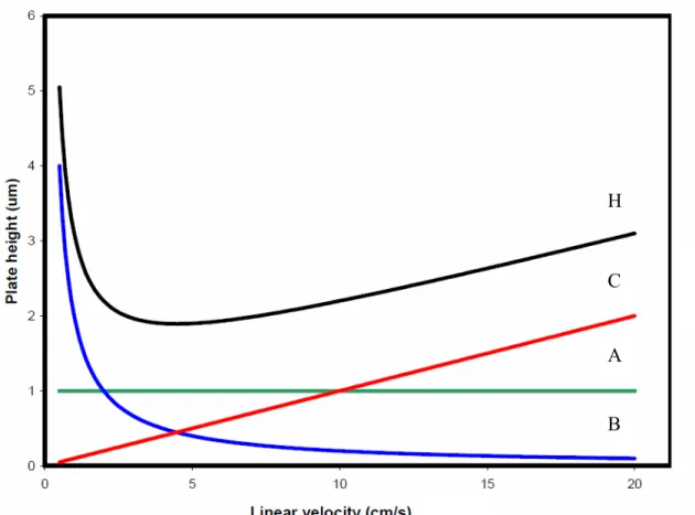
Figure 1-1: Theoretical relationship between the A-, B-, and C-term of the van
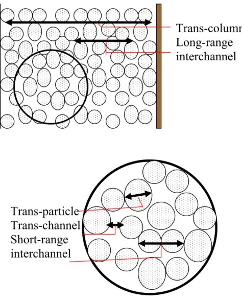
Deemter equation... 30 Figure 1-2: Diagram of the location and distance of the different contributions
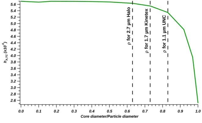
to eddy dispersion in a packed column ... 31 Figure 1-3: Theoretical relationship between the porous layer thickness and
the HA,TC-term. p1/q1 = 8/225, ml = 150,000, mr = 15, *β,c = 1.5%, T = 0.65,
i = 0.40, k’ = 2, r = 0.3 ... 32
Figure 1-4 Theoretical relationship between HA (total) and the porous layer
thickness. p1/q1 = 8/225, ml = 150,000, mr = 15, *β,c = 1.5%, T = 0.65, i =
0.40, k’ = 2, r = 0.3 ... 33
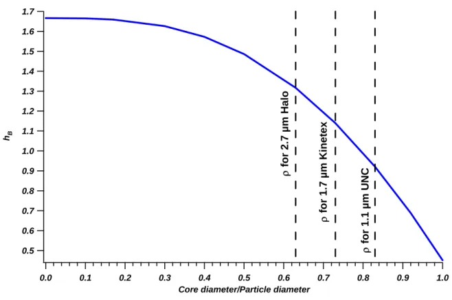
Figure 1-5: Theoretical relationship between the porous layer thickness and
the B-term. i = 0.40, 2 = 0.3277, and = 1 ... 34
Figure 1-6: Theoretical relationship between the trans-particle (porous layer thickness and the liquid stationary phase and stagnant mobile phase)
resistance to mass transfer. K = 0.5, Sh = 10, εi= 0.40, k1 varies as a function
of ... 35 Figure 1-7: Theoretical relationship between the porous layer thickness and
the mobile phase resistance to mass transfer. εi = 0.40 and k1 varies with
porous layer thickness... 36 Figure 1-8: Theoretical relationship between the porous layer thickness and
the theoretical plate height at v = 3 ... 37 Figure 1-9: Theoretical relationship between the theoretical plate height and
linear velocity at varying porous layer thickness for a small molecules analyte
(DM = 1 x 10⁻⁵). dp =1.0 m ... 38
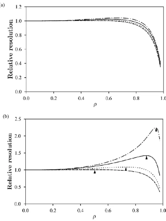
Figure 1-10: Reduced plate heights of compounds having different molecular sizes as a function of reduced velocity, for different porous layer thickness. = 1: solid line, = 0.85: dot-dashed line, = 0.7: dashed line, = 0.5: dotted line, = 0: thick solid line. (a) small molecule; (b) medium-sized peptide; (c)
large peptide; (d) protein.[35] ... 39 Figure 1-11: Resolution of pairs of compounds having different molecular
a column packed with fully porous particles. (a) Resolution calculated at the optimum linear velocity for the analyte of interest (b) Resolution calculated at
the optimum linear velocity for small molecules.[35] ... 40 Figure 1-12: Effect of decreasing particle diameter on efficiency. Dm = 1.0 x
10-5 cm2/sec and dp = 1.0 m ... 41
Figure 2-1: Structure of poly(diallydimethylammonium chloride... 100 Figure 2-2: Diagram of particle sieving device. F1 and F3 are 2 m
polycarbonate membrane filters and F2 is a 3 m polycarbonate membrane
filter.[48] ... 101 Figure 2-3: Images of the coating process. A) NPS, B) 1 full coating step, C)
3 full coating steps, D) 5 full coating steps, E) 10 full coating steps. 1.4 m NPS core (Eprogen), 0.5%(w/w%) HMW PDDA, 10% (w/w%) Nalco 1034A
(20 nm) colloidal silica ... 102 Figure 2-4: Particle size distribution of 1.4 m core particles after 10 coating
steps... 103 Figure 2-5: Comparison of Superficially Porous Particles after A1) wide view
of 10 coating step particles, A2) close view of 10 coating step particles, B1)
wide view of 5 coating step particles, and B2) close view of 5 coating step
particles. 1.4 m NPS core (Eprogen), 0.5% (w/w%) HMW PDDA, 10%
(w/w%) Nalco 1034A (20 nm) colloidal silica ... 104 Figure 2-6: Particle size distribution of 1.4 m core particles after 5 coating
steps... 105 Figure 2-7: Growth Rate Comparison Based on Number of Coating Steps. (
) 5 Coating Step Preparation ( ) 10 Coating Step Preparation ... 106 Figure 2-8: Particle size distribution of the 10 coating layer particles after
sizing using the reversible flow sieving device ... 107 Figure 2-9: Comparison of particles sized with particle filtration apparatus. A)
before filtering, B) within region 3 (2-3 m), C) within region 2 (> 3 m). 1.4
m NPS core (Eprogen), 10 alternating layers of 0.5% (w/w%) HMW PDDA
and 10% (w/w%) Nalco 1034A (20 nm) colloidal silica... 108 Figure 2-10: Comparison of particles sized with top loaded filtration apparatus
. A) before filtering, B) removal of particles with 2.0 m Nylon filter, C) removal of particles larger than 5 m with nylon filter. 1.4 m NPS core (Eprogen), 10 alternating layers of 0.5% (w/w%) HMW PDDA and 10%
Figure 2-11: Diagram of theoretical polyelectrolyte orientation on NPS. A) Polyelectrolyte perpendicular to the NPS surface, B) polyelectrolyte parallel
to the NPS surface... 110 Figure 2-12: Comparison of polyelectrolyte molecular weight. A) one coat
0.5% (w/w%) LMW PDDA and 10% (w/w%) Nalco 1034A (20 nm), B) three alternating coats of 0.5% (w/w%) LMW PDDA and 10% (w/w%) Nalco 1034A (20 nm), C) one coat 0.5% (w/w%) HMW PDDA and 10% (w/w%) Nalco 1034A (20 nm), D) three alternating coats of 0.5% (w/w%) HMW
PDDA and 10% (w/w%) Nalco 1034A (20 nm) colloidal silica ... 111 Figure 2-13: Diagram of effect of polyelectrolyte molecular weight on surface
thickness variations and roughness. (A) HMW, side view (B) LMW, side view... 112 Figure 2-14: Effect of the number of polyelectrolyte washes on the surface
uniformity and webbing between particles. A) One full layer B) two full layers C) three full layers 1.4 m NPS (Eprogen), 0.5% (w/w%) LMW
PDDA, 10% (w/w%) AS-30 (12 nm) colloidal silica... 113 Figure 2-15: Effect of polyelectrolyte concentration (w/w%). A) 0.5%, B)
0.25%, C) 0.1%, D) 0.05%. 1.4 m NPS (Eprogen), coated with three
alternating layers of LMW PDDA and Nalco 1034A (20 nm) colloidal silica ... 114 Figure 2-16: Effect of polyelectrolyte concentration (w/w%). A) 0.5%, B)
0.25%, C) 0.1%, D) 0.05%. 1.4 m NPS (Eprogen), coated with one
alternating layer of LMW PDDA and Ludox AS-30 (12 nm) colloidal silic ... 115 Figure 2-17: Comparison of colloidal silica stabilization pH. A) 10% (w/w%)
Nalco 1034A (20 nm), pH = 2.8, B) 10% (w/w%) Nalco 1030 (13 nm), pH = 10.2. 1.4 m NPS (Eprogen), coated with three alternating layers of 0.5%
(w/w%) LMW PDDA and colloidal silica... 116 Figure 2-18: Comparison of colloidal silica size. A) NexSil 8 (8 nm), B)
Nalco 1030 (13 nm), C) NexSil 85 (85 nm), D) NexSil 125 (125 nm). 1.4 m NPS (Eprogen), coated with one alternating layer of 0.5% (w/w%) LMW
PDDA and 10% (w/w%) colloidal silica ... 117 Figure 2-19: Comparison of solution mixing method. A) Centrifuge tube
mixing, B) Beaker with stir bar mixing. 1.4 m NPS (Eprogen), coated with three alternating layers of 0.5% (w/w%) LMW PDDA and 10% (w/w%)
Nalco 1030 (13 nm) colloidal silica... 118 Figure 2-20: SEM image of NPS starting material indicating the presence of
alternating layers of 0.5% (w/w%) LMW PDDA and 10% (w/w%) Nalco
1030 (13 nm) colloidal silica ... 120 Figure 2-22: Comparison of sintering temperature. A) 855˚C, B) 900˚C, C)
950˚C, D) 980˚C, E) 990˚C. 1.4 m NPS (Eprogen), coated with three alternating layers of 0.5% (w/w%) LMW PDDA and 10% (w/w%) Nalco
1030 (13 nm) colloidal silica ... 121 Figure 2-23: Comparison of sintering temperature effect on particle
mechanical strength. Sonication of 3 mg/mL aqueous slurry solutions ... 122 Figure 2-24: Comparison of surface melting when sintered at 980˚C. A) Batch
1 B) Batch 2. Both batches used the same NPS core particles, 0.5% (w/w%)
LMW PDDA solution, and 10% (w/w%) Nalco 1030 (13 nm) solution... 123 Figure 2-25: Comparison of surface melting when sintered at 980˚C. A) Batch
1 B) Batch 2. Both batches used the same NPS core particles, 0.5% (w/w%)
LMW PDDA solution, and 10% (w/w%) Ludox AS-30 (12 nm) solution ... 124 Figure 2-26: Chromatogram for Column LB1-68 at the optimum linear
velocity. Particles with 10 coating layers, bonded with C18, and singly endcapped. 30 m i.d. x 12.5 cm, run in 70/30 water/ACN 0.1% TFA, hmin
(HQ) = 3.0, uopt = 0.06 cm/sec (5600 psi), k’ (4MC) = 0.61 ... 125
Figure 2-27: Reduced parameters plot for Column LB1-68. Particles with 10 coating layers, bonded with C18, and singly endcapped. 30 m i.d. x 12.5 cm, run in 70/30 water/ACN 0.1% TFA, hmin (HQ) = 3.0, uopt = 0.06 cm/sec (5600
psi), k’ (4MC) = 0.61 ... 126 Figure 2-28: Reduced parameters plot for Column LB6-1. 1.9 m Acquity
C18 particles, 30 m i.d. x 19.8 cm, run in 50/50 water/ACN 0.1% TFA, hmin
(HQ) = 1.2, uopt = 0.19 cm/sec (6600 psi), k’ (4MC) = 0.53 ... 127
Figure 2-29: Chromatogram for Column LB1-95 at the optimum linear velocity. Particles with 5 coating layers, bonded with C18, and singly endcapped. 30 m i.d. x 24.3 cm, run in 70/30 water/ACN 0.1% TFA, hmin
(HQ) = 1.7, uopt = 0.13 cm/sec (8900 psi), k’ (4MC) = 0.45 ... 128
Figure 2-30: Reduced parameters plot for Column LB1-95. Particles with 5 coating layers, bonded with C18, and singly endcapped. 30 m i.d. x 24.3 cm, run in 70/30 water/ACN 0.1% TFA, hmin (HQ) = 1.7, uopt = 0.13 cm/sec (8900
psi), k’ (4MC) = 0.45 ... 129 Figure 2-31: Chromatogram for Column LB1-103B at the optimum linear
velocity. Particles with 5 coating layers, bonded with C18, and doubly endcapped. 30 m i.d. x 28.3 cm, run in 70/30 water/ACN 0.1% TFA, hmin
Figure 2-32: Reduced parameters plot for Column LB1-103B. Particles with 5 coating layers, bonded with C18, and doubly endcapped. 30 m i.d. x 28.3 cm, run in 70/30 water/ACN 0.1% TFA, hmin (HQ) = 3.9, uopt = 0.03 cm/sec
(2400 psi), k’ (4MC) = 0.48... 131 Figure 2-33: SEM images indicating particle structural degradation. A) intact
column bed, B) free particles from extruded bed, C) particles after boding and endcapping. 1.4 m NPS (Eprogen), coated with three alternating layers of 0.5% (w/w%) LMW PDDA and 10% w/w%) Nalco 1034A (20 nm) colloidal
silica ... 132 Figure 2-34: Comparison of the particle surface roughness. A) 2.6 m Kinetex
B) 5 layer particles ... 133 Figure 2-35: Comparison of original 1.7 m particles (A) and particles with
revised conditions based on experimentation contained within this chapter (B)... 134 Figure 2-36: Particle size distribution of 1.4 m core particles after 3 coating
steps with revised synthesis parameters determined within this chapter... 135 Figure 2-37: Illustration of the ring structure of the porous layer of 1.7 m
Kinetex particles. ... 136 Figure 2-38: Hydroquinone chromatographic performance comparison of 5
layer particles and particles synthesized by the revised conditions. 30 m i.d.
columns run in 70/30 water/ACN with 0.1% TFA ... 137 Figure 3-1: Theoretical curves for the contributions to the c term versus k’ for
an analyte. The blue trace is for the stagnant mobile phase term. The red trace is for the mobile phase term. The green trace is for the resistance to mass transfer in the stationary phase. The black trace is the total contribution to the
c term as it varies with k’.[31... 183
Figure 3-2: Polyelectrolyte structures... 184 Figure 3-3: SEM image of the particle agglomeration seen in the initial
synthesis of 1.1 m superficially porous particles... 185 Figure 3-4: Effect of NPS core solution pH on surface coverage. One coating
step, 0.9 m NPS (Eprogen (Darien, IL)), 0.5% (w/w%) LMW PDDA, 10%
(w/w%) AS-30 (20 nm) colloidal silica (pH = 3.5). (A) pH = 2.3; (B) pH = 5.5... 186 Figure 3-5: Diagram of effect of polyelectrolyte molecular weight (chain
Figure 3-7: Effect of molecular weight of polyelectrolyte. Three coating steps, 0.9 m NPS (Fiber Optic Center), 0.5% (w/w%) polyelectrolyte, 10%
(w/w%) AS-30 (pH = 3.5). ... 189 Figure 3-8: Diagram of effect of polyelectrolyte molecular weight on surface
thickness variations and roughness. (A) HMW, side view (B) LMW, side view... 190 Figure 3-9: Effect of polyelectrolyte type on surface coverage and uniformity.
A) LMW PDDA B) HMW PDDA C) PEI D) LMW PAH E) HMW PAH... 191 Figure 3-10: Effect of polyelectrolyte concentration (w/w%) on surface
coverage. One coating step, 0.9 m NPS (Fiber Optic Center), LMW PDDA,
10% (w/w%) AS-30 (pH = 3.5). (A) 1.0%; (B) 0.5%; (C) 0.1%; (D) 0.05... 192 Figure 3-11: Diagram of effect of ionic strength on polyelectrolyte
conformation and colloidal silica layer thickness. (A) low ionic strength, top view; (B) high ionic strength, top view; (C) low ionic strength, side view; (D)
high ionic strength, side view ... 193 Figure 3-12: Effect of salt concentration on surface coverage, uniformity, and
roughness. Two coating steps, 0.9 m NPS (Eprogen (Darien, IL)), 0.5% (w/w%) LMW PDDA, 10% (w/w%) AS-30 (pH = 3.5). (A) 0.0 M NaCl; (B)
0.2 M NaCl; (C) 0.4 M NaCl; (D) 0.6 M NaCl ... 194 Figure 3-13: Comparison of colloidal silica size. One coating step, 0.9 m
NPS (Fiber Optic Center), 0.5% (w/w%) LMW PDDA, 10% (w/w%) colloidal silica (pH = 3.5). (A) Nyacol Nexsil125 (125 nm); (B) Nyacol NexSil85 (85 nm); (C) Nalco 1060 (60 nm); (D) Nalco 1030 (13 nm); (E)
Aldrich, AS-30 (12 nm); (F) Nyacol, NexSil8 (8 nm)... 195 Figure 3-14: Effect of colloidal silica solution pH on NPS core surface
coverage. One coating step, 0.9 m NPS (Eprogen), 0.5% (w/w%) LMW PDDA, 10% (w/w%) AS-30 (20 nm) colloidal silcia. (A) pH = 3.5; (B) pH =
9.4... 196 Figure 3-15: Effect of drying method on particle coverage and uniformity.
Three coating steps, 0.9 m NPS (Fiber Optic Center), 0.5% (w/w%) LMW PDDA, 10% (w/w%) AS-30 (20 nm) colloidal silica (pH = 3.5). (A) Dried at
25C; (B) Dried at 80C; (C) Dried at 105C; (D) Lyophilized... 197 Figure 3-16: Particle degradation seen from extruded column bed. Three
coating steps, 0.9 m NPS (Eprogen (Darien, IL)), 0.5% (w/w%) LMW PDDA, 10% (w/w%) Nalco 1030 (13 nm) colloidal silica (pH = 3.5), sintered
at 825C, bonded and endcapped... 198 Figure 3-17: Particle size distribution of 1.1 m (dp,n) superficially porous
Figure 3-18: Example chromatogram for column LB3-104, particles LB3-102-1 bonded by U.S. patent 20020070LB3-102-168. Packed in acetone at 3 mg/mL. Mobile phase: 80/20 water/ACN 0.1% TFA, uopt = 0.05 cm/sec (8300 psi) hmin (HQ) =
4.3, k’ (4MC) = 0.9 ... 200 Figure 3-19: Reduced parameters plot for column 104, particles
LB3-102-1 bonded by U.S. patent 20020070168. Packed in acetone at 3 mg/mL. Mobile phase: 80/20 water/ACN 0.1% TFA, uopt = 0.05 cm/sec (8300 psi).
hmin (HQ)= 4.3, k’ (4MC) = 1.2 ... 201
Figure 3-20: Images of Column LB3-104 extruded bed. A) image of column cross-section near column outlet where red circles highlight column voids B)
expanded section of column cross-section... 202 Figure 3-21: Example chromatogram comparison of different bonding and
endcapping procedures. Mobile phase: 80/20 water/ACN 0.1% TFA. A) U.S. patent 20020070168, tri-functional silane, uopt = 0.08 cm/sec (6900 psi), hmin
(HQ) = 3.7, k’ (4MC) = 1.3. B) U.S. patent 20100076103, mono-functional
silane, uopt = 0.12 cm/sec (6600 psi), hmin (HQ) = 2.2, k’ (4MC) = 1.3... 203
Figure 3-22: Reduced parameters plot for hydroquinone comparing different bonding and endcapping procedures. U.S. patent 20020070168, tri-functional silane: uopt = 0.08 cm/sec (6900 psi), hmin (HQ)= 3.7, k’ (4MC) = 1.3. U.S.
patent 20100076103, mono-funtional silane: uopt = 0.12 cm/sec (6600 psi),
hmin (HQ) = 2.2, k’ (4MC) = 1.3. ... 204
Figure 3-23: Diagrams of proposed bonding agent attachment. A)
mono-functional silane, no polymerization, B) tri-mono-functional siliane, polymerization ... 205 Figure 3-24: Reduced parameters plot for hydroquinone comparing the effect
of the column inner diameter on column performance. Columns LB3-117 (30
m i.d.) and LB3-122 (20 m i.d.), LB3-104-3 particles bonded and endcapped using U.S. patent 20020070168, tri-functional silane, packed in solvent X. Mobile phase: 80/20 water/ACN 0.1% TFA. LB3-117: uopt = 0.03
cm/sec (3600 psi), hmin (HQ) = 6.3, k’ (4MC) = 0.58. LB3-122: uopt = 0.06
cm/sec (5100 psi), hmin (HQ) = 3.7, k’ (4MC) = 1.4... 206
Figure 3-25: Reduced parameters plot for hydroquinone comparing the effect of the column inner diameter on column performance. Columns LB3-153 (30
m i.d.) and LB4-12-C (20 m i.d.), LB3-133-2 particles bonded and endcapped using U.S. patent 20020070168, tri-functional silane, packed in methanol. Mobile phase: 80/20 water/ACN 0.1% TFA. LB3-153: uopt = 0.13
cm/sec (7000 psi), hmin (HQ) = 2.9, k’ (4MC) = 1.1. LB4-12-C: uopt = 0.13
20020070168, tri-functional silane. Mobile phase: 80/20 water/ACN 0.1%
TFA. ... 208 Figure 3-27: Effect of packing pressure on k’. ... 209 Figure 3-28: Effect of packing pressure on chromatographic performance.
Particles LB3-133-2, bonded and endcapped with U.S. patent 20020070168, tri-functional silane, packed in methanol. Mobile phase: 80/20 water/ACN
0.1% TFA... 210 Figure 3-29: Reduced parameters plot comparing columns packed with
particles synthesized in-house to those of commercial particles. ... 211 Figure 3-30: SEM images of 1.7 m Kinetex particles showing the presence
of particle multiplets. ... 212 Figure 4-1: Comparison of predicted values for small molecules (Dm = 1 x 10
-5 cm2/sec) for totally porous particles, superficially porous particles, and
non-porous particles ... 244 Figure 4-2: Particle size distribution of 1.1 m (dp,n) particles coated with 12
nm colloidal silica. RSD = 2.1%... 245 Figure 4-3: Particle size distribution of 1.1 m (dp,n) particles coated with 28
nm colloidal silica. RSD = 3.8%... 246 Figure 4-4: Particle size distribution of 1.6 m (dp,n) particles coated with 67
nm colloidal silica. RSD = 3.8%... 247 Figure 4-5: Images of particles coated with varying diameter of colloidal
silica. A) 1.1 m (dp,n) with 12 nm colloidal silica B) 1.1 m (dp,n) with 28
nm colloidal silica C) 1.6 m (dp,n) with 67 nm colloidal silica... 248
Figure 4-6: CPS Disc Centrifuge raw data for the 1.1 m (dp,n), 12 nm
colloidal silcia. ... 249 Figure 4-7: CPS Disc Centrifuge raw data for the 1.1 m (dp,n), 28 nm
colloidal silica. ... 250 Figure 4-8: CPS Disc Centrifuge raw data for the 1.6 m (dp,n), 67 nm
colloidal silica. ... 251 Figure 4-9: Example chromatograms for superficially porous particles of
varying pore size for analysis of small molecules. A) Column LB7-32, LB6-75-1 particles (1.1 m (dp,n)), 12 nm colloidal silica C18 bonded, 30 m x
16.9 cm, MP: 80/20 water/ACN 0.1% TFA, hmin (HQ) = 2.6, uopt = 0.09
m), 28 nm colloidal silica C18 bonded, 30 m x 12.8 cm, MP: 80/20 water/ACN 0.1% TFA, hmin (HQ) = 2.6, uop t = 0.16 cm/sec (8700 psi),
k’(4MC) = 1.3 ... 252 Figure 4-10: Example chromatogram for large pore superficially porous
particles. Column LB7-23-C, LB6-111-3 particles (1.6 m (dp,n)), 67 nm
colloidal silica, C18 bonded, 30 m x 12.3 cm, MP: 90/10 water/ACN 0.1%
TFA, hmin (HQ) = 3.3, uopt = 0.08 cm/sec (2500 psi), k’(4MC) = 0.9... 253
Figure 4-11: Reduced parameters plot comparison for superficially porous
particles with varying pore size fit to the van Deemter equation. ... 254 Figure 4-12: Example chromatograms for 1.6 m (dp,n), 67 nm coated
superficially porous particles. A) Column LB6-112, LB6-102-6 particles, C18 bonded, 30 m x 13.8 cm, MP: 90/10 water/ACN 0.1% TFA, hmin (HQ) = 3.7,
uopt = 0.06 cm/sec (2300 psi), k’(4MC) = 0.7 B) Column 146-B,
LB6-138-4 particles, C8 bonded, 30 m x 13.4 cm, MP: 90/10 water/ACN 0.1%
TFA, hmin (HQ) = 3.6, uopt = 0.07 cm/sec (2300 psi), k’(4MC) = 0.8... 255
Figure 4-13: Example chromatograms for 1.6 m (dp,n), 67 nm coated
superficially porous particles. C18 Bonded) Column LB6-112, LB6-102-6 particles, C18 bonded, 30 m x 13.8 cm, MP: 90/10 water/ACN 0.1% TFA, hmin (HQ) = 3.7, uopt = 0.06 cm/sec (2300 psi), k’(4MC) = 0.7 C8 Bonded)
Column LB6-146-B, LB6-138-4 particles, C8 bonded, 30 m x 13.4 cm, MP: 90/10 water/ACN 0.1% TFA, hmin (HQ) = 3.6, uopt = 0.07 cm/sec (2300 psi),
k’(4MC) = 0.8. ... 256 Figure 4-14: Example chromatograms for superficially porous particles of
varying pore size for analysis of peptides of enolase digest. A) Column LB7-41, LB6-75-1 particles, C18 bonded, 75 m x 16 cm B) Column LB7-41-B, LB7-23-3 particles, C18 bonded, 75 m x 15 cm C) Column 111,
LB6-111-3 particles, C18 bonded, 75 m x 27 cm... 257 Figure 4-15: Example chromatogram of in-house superficially porous particles
compared to non-porous particles and totally porous particles for analysis of peptides of enolase digest. A) Column LB6-150, 1.5 m NPS, C18 bonded, 75
m x 17 cm B) Column LB7-41, LB6-75-1 particles, C18 bonded, 75 m x 16
cm C) Waters 1.9 m Acquity BEH130, 75 m x 25 cm... 258 Figure 4-16: Example chromatograms for enolase digest separated using 1.6
m particles coated with 85 nm colloidal silica variation in bonded ligand chain length. A) Column LB6-111, LB6-111-3 particles, C18 bonded, 75 m x 27 cm B) Column LB6-146, LB6-138-4 particles, C8 bonded, 75 m x 25
Figure 4-17: Example chromatogram for superficially porous particles of varying pore size for analysis of protein mixture. Mixture included thyroglobulin (1), -lactogloulin (2), RNasa-A (3), cytochrome c (4), myoglobin (5), bovine serum albumin (6) A) Column LB7-41, LB6-75-1 particles, C18 bonded, 75 m x 16 cm B) Column LB7-41-B, LB7-23-3 particles, C18 bonded, 75 m x 15 cm C) Column LB6-111, LB6-111-3
particles, C18 bonded, 75 m x 27 cm ... 260 Figure 4-18: 3D plot for 87 Å pore particles ... 261 Figure 4-19: 3D plot for 1.5 m NPS particles, C18 bonded. ... 262 Figure 4-20: 3D plot for 187 Å pore particles ... 263 Figure 4-21: 3D plot for 248 Å pore particles bonded with C18... 264 Figure 4-22: Example chromatograms for protein mixture separated using 1.6
m particles coated with 85 nm colloidal silica variation in bonded ligand chain length. Mixture included thyroglobulin (1) RNasa-A (2) cytochrome c (3) myoglobin (4) -lactogloulin (5) bovine serum albumin (6) A) Column LB6-111, LB6-111-3 particles, C18 bonded, 75 m x 27 cm B) Column
LB6-146, LB6-138-4 particles, C8 bonded, 75 m x 25 cm ... 265 Figure 4-23: 3D plot for 248 Å pore particles bonded with C8... 266 Figure 5-1: Example of sedimentation rate and effective particle size
measurement set-up. A) acetone B) methanol C) tetrahydrofuran D) hexane E)
isopropanol... 298 Figure 5-2: Images of 1.1 m (dp,n) particles coated with 12 nm colloidal silica
by in-solution microscopy. A) acetone B) methanol C) hexane D) solvent X ... 299 Figure 5-3: Images of 1.1 m (dp,n) particles coated with 28 nm colloidal silica
by in-solution microscopy. A) acetone B) methanol C) hexane D) solvent X ... 300 Figure 5-4: Images of 1.1 m (dp,n) particles coated with 28 nm colloidal silica
by in-solution microscopy in methanol at varying concentrations. A) 25
mg/mL B) 13 mg/mL C) 7 mg/mL D) 3 mg/mL ... 301 Figure 5-5: Images of 1.1 m (dp,n) particles coated with 28 nm colloidal silica
by in-solution microscopy in acetone at varying concentrations. A) 25 mg/mL
B) 13 mg/mL C) 7 mg/mL ... 302 Figure 5-6: Example chromatograms for columns packed with 1.1 m (dp,n)
particles coated with 28 nm colloidal silica in varying slurry solvent. A) acetone, Column LB6-81, LB6-57-4 particles, 30 m x 11.6 cm, hmin (HQ) =
LB6-153-C, LB6-57-4 particles, 30 m x 12.5 cm, hmin (HQ) = 3.5, uopt = 0.07
cm/sec (4400 psi), k’(4MC) = 1.04... 303 Figure 5-7: Example chromatograms for columns packed with 1.1 m (dp,n)
particles coated with 28 nm colloidal silica in varying slurry solvent. A) hexane, Column LB7-20, LB6-57-4 particles, 30 m x 10.2 cm, hmin (HQ) =
6.1, uopt = 0.06 cm/sec (3000 psi), k’(4MC) = 1.06 B) solvent X, Column
LB6-153-A, LB6-57-4 particles, 30 m x 12.6 cm, hmin (HQ) = 6.8, uopt = 0.03
cm/sec (1800 psi), k’(4MC) = 0.98... 304 Figure 5-8: Reduced parameters plot comparison for columns packed with 1.1
m (dp,n) particles coated with 28 nm colloidal silica in varying slurry solvent.
A) acetone B) methanol C) hexane D) solvent X ... 305 Figure 5-9: Example chromatograms for columns packed with 1.1 m (dp,n)
particles coated with 28 nm colloidal silica at varying slurry concentration. A) Column LB7-38, LB7-23-3 particles, slurry concentration = 3 mg/mL, 30 m x 10.2 cm, hmin (HQ) = 4.8, uopt = 0.06 cm/sec (2600 psi), k’(4MC) = 1.2 B)
Column LB7-33, particles LB7-23-3, slurry concentration = 25 mg/mL, 30
m x 12.8 cm, hmin (HQ) = 2.6, uopt = 0.16 cm/sec (8700 psi), k’(4MC) = 1.3... 306
Figure 5-10: Reduced parameters plot comparison of hydroquinone for
columns packed with 1.1 m (dp,n) particles coated with 28 nm colloidal silica
at varying slurry concentration fit to the van Deemter equation. ... 307 Figure 5-11: Images of 28 nm colloidal silica coated particles prepared by
different washing methods. A) Centrifuged B) Settled ... 308 Figure 5-12: Example chromatograms for columns packed with centrifuge
washed particles and settle washed 1.1 m (dp,n), 28 nm coated particles. A)
Column LB7-33, LB7-23-3 particles, 30 m x 12.8 cm, hmin (HQ) = 2.6, uopt =
0.16 cm/sec (8700 psi), k’(4MC) = 1.3 B) Column LB7-49, LB7-114-3 particles, 30 m x 12.6 cm, hmin (HQ) = 2.3, uopt = 0.17 cm/sec (8300 psi),
k’(4MC) = 1.0 ... 309 Figure 5-13: Reduced parameters plots for hydroquinone for columns packed
with centrifuge washed particles and settle washed 1.1 m (dp,n), 28 nm
LIST OF ABBREVIATIONS
ACN Acetonitrile
BEH Ethylene Bridged Hybrid
BET Brunauer, Emmett, and. Teller
BSA Bovine Serum Albumin
C Catechol
Cm Resistance to mass transfer in the mobile phase
C4 n-butyl
C8 n-octyl
C18 n-octadecyl
DI Deionized
DLS Dynamic Light Scattering
DLS PDI Dynamic Light Scattering Polydispersity Index
ESI Electrospray ionization
FCS Colloidal silica footprint
HMW PAH High Molecular Weight Poly(allylamine hydrochloride)
HMW PDDA High Molecular Weight Poly(diallydimethyl ammonium chloride) HPLC High Pressure Liquid Chromatography
HQ Hydroquinone
IPA Isopropanol
IT Short-range interchannel
LMW PDDA Low Molecular Weight Poly(diallydimethyl ammonium chloride)
LC Liquid Chromatography
MeOH Methanol
MW Molecular Weight
m/z mass-to-charge ratio
NPS Non-Porous Silica
PDI Polydispersity Index
PEI Poly(ethylamine)
PTFE Polytetrafluoroethylene
Q-TOF Quadrupole-Time of Flight
R Resorcinol
RSD Relative Standard Deviation
SEM Scanning Electron Microscope
SPP Superficially Porous Particle
SSA Specific Surface Area
StDef Filter Standard Definition Filter
TC Trans-column
TEAP triethylammonium phosphate
TEOS tetraethyl-orthosilicate
TFA trifluoroacetic acid
THF Tetrahydrofuran
UHPLC-MSE Ultrahigh Pressure Liquid Chromatography-Mass SpectrometryE
LIST OF SYMBOLS
A Eddy dispersion van Deemter coefficient
a Reduced eddy dispersion van Deemter coefficient AIT Short-range interchannel contribution to the A-term
ALRI Long-range interchannel contribution to the A-term
ATC Trans-column contribution to the A-term
ATP Trans-particle contribution to the A-term
ATS Trans-channel contribution to the A-term
Degree of aggregation
B Longitudinal diffusion van Deemter coefficient
b Reduced longitudinal diffusion van Deemter coefficient
Diffusion coefficient scalar parameter to account for varying particle porous layer thickness
Packing structure parameter
Bonded phase surface coverage
C Resistance to mass transfer van Deemter coefficient
CAT Aris-Taylor coefficient
Cf External (eluent) film resistance to mass transfer for superficially
porous particles
CM Resistance to mass transfer in the mobile phase van Deemter
coefficient
CMSt Resistance to mass transfer in the stagnant mobile phase van Deemter
coefficient
CS Resistance to mass transfer in the stationary phase van Deemter
coefficient
c Reduced resistance to mass transfer van Deemter coefficient
%C Percent carbon (w/w%)
D Diffusion coefficient
dcs Colloidal silica diameter
dcore Diameter of core particle
dc/dp Diameter of core to total diameter of particle, aspect ratio
Deff Effective diffusion coefficient
deff Effective particle diameter
df Liquid stationary phase thickness
Dm Diffusion of analyte in the mobile phase
Dp Particle diffusivity across the porous stationary phase
dp Total particle diameter
dp,i Individual particle diameter
dp,n Number average particle diameter
dpore Pore diameter
dp,v Volume average particle diameter
DS Diffusion coefficient in the stationary phase
ds Stationary phase file thickness
Intraparticle porosity
f Particle porosity filled with solvent
i Interparticle porosity
εp Particle porosity
εT Total column porosity
g Gravitational constant
’ Tortuosity factor
m Obstruction factor in the mobile phase
r Coefficient related to the contribution of eluent convection to the
radial dispersion of the sample
S Obstruction factor in the stationary phase
Viscosity
H Height equivalent to a theoretical plate
HA Height equivalent to a theoretical plate due to eddy dispersion
HB Height equivalent to a theoretical plate due to longitudinal diffusion
HC Height equivalent to a theoretical plate due to resistance to mass
transfer
Hdiffusion Diffusion contribution to the coupled A-term
Hflow Flow contribution to the coupled A-term
Hheat Heat of friction contribution to the theoretical plate height
Hmin Minimum theoretical plate height
hmin Reduced theoretical plate height
h Reduced theoretical plate height
K Henry’s constant
K2 particle-solvent dependant constant
kf External film mass transfer coefficient
k1 Zone retention factor
L Column length
Scaling factor for the A-term contribution based on the van Deemter equation
i Structural parameter for the A-term based on the Giddings equation IT Short-range interchannel structural parameter
TC Trans-column structural parameter
ml Column length/column inner diameter
mr Column inner radiusr/particle diameter
MW Molecular weight
N Number of theoretical plates
NC Number of coating steps
nC Number of carbons in the bonding ligand
ni Number of particles with a specific particle diameter
Np Number of particle in column
Effective diffusivity of the analyte in the porous shell to the bulk diffusion coefficient
Pc Peak capacity
P Change in pressure
Popt Pressure required to obtain the optimum flow rate
p1/q1 Factor to account for the concentration of the sample in the stationary
phase as compared to the total column
Fraction of mobile phase stagnant in the particle pores
p Volume fraction of the particles
Intraparticle tortuosity
r Layer thickness growth rate
Rcs Ratio of pore diameter to colloidal silica diameter
Re Reynolds number
rH Hydrodynamic radius
Rs Resolution
Core diameter/total particle diameter
skel Density of the particle skeleton
l Density of the solvent
SACS Surface area of colloidal silica particle
SANPS Surface area of NPS particle
SAV Surface area per column volume
SAtotal Total surface area of a superficially porous particle
Sc Schmidt number
Sh Sherwood number
SSA Specific surface area
T Temperature
Tf Tailing factor
to Void time (dead time)
tr Retention time
t Length of gradient in time units
tR Retention time difference between critical pair
u Linear velocity
u0 Superficial linear velocity
uopt Optimum linear velocity
V Total particle volume
v Reduced linear velocity
Vc Total column volume
vexperimental Experimentally obtained sedimentation velocity
vextreme Linear velocity of mobile phase a higher or lower value than the mean
linear velocity
vmean Mean mobile phase linear velocity
VMP Volume of mobile phase per column volume
Vp Volume of column occupied by particles
Vpore Pore volume per particle
vS Sedimentation velocity
VSP Volume of stationary phase per column volume
%Vcore Percent of the total particle volume that is occupied by the solid core
%Vporous Percent of the total particle volume that is porous
vtheoretical Theoretically obtained sedimentation velocity
WC,p Weight of carbon per particle
WC,v Weight of carbon per column volume
wfront,5% Front half peak width
Wp Weight of one particle
wt,i 4 peak width
Ratio of the exchange distance to the particle diameter between
velocity extremes
Fractional departure of the velocity extreme from the mean value i Structural parameter for the A-term based on the Giddings equation IT Short-range interchannel structural parameter
Structural parameter typically near unity
TC Trans-column structural parameter
,c* Relative velocity difference between the center and the wall of the
column
CHAPTER 1: INTRODUCTION
1.1 SUPERFICIALLY POROUS PARTICLES 1.1.1 Historical Background
Pellicular particles were introduced by Horvath et. al. to carry out highly efficient separations with lower pressure requirements for fast analyses.[1,2] Following this initial development, Dupont, Merck, and Waters Inc. developed similar materials for use with liquid chromatography.[3-5] The products were commercialized as Zipax, Perisorb, and Corasil, respectively, which had particle diameters around 40 m.[4,6] Initially, superficially porous particles showed significant advantages over similarly sized totally porous particles, but in the mid-1970’s these materials became overshadowed by development of smaller diameter, spherical, totally porous particles.[7,8] Not until recently have superficially porous particles again attracted attention.
Halo, which has a particle diameter of 2.7 m and a pore diameter of 80Å.[10] Following the introduction of Halo particles, similarly sized particles such as Kinetex, Ascentis Express, Poroshell, and Accucore were introduced by Phenomenex, Supelco, Agilent Technologies, and Thermo Fisher, respectively. Based on earlier work, Agilent Technologies varied this procedure to produce 5.0 m Poroshell particles with 300 Å pores.[3] Others followed with the production of particles suitable for proteins, such as Halo-ES and Aeris WIDEPORE by Advanced Materials Technology and Phenomenex, respectively.
1.1.2 Synthesis Methods
Since the initial development of superficially porous particles by Horvath, several production methods have been employed. One improvement was to modify the layer-by-layer method developed by Kirkland to include spray-drying to produce highly uniform particles.[11] Alternatively, the method employed by Büchel et. al. forms superficially porous particles by adding a tetraethyl-orthosilicate (TEOS)/porogen mixture to a suspension of non-porous silica (NPS) cores. The porogen, n-octadecyltrimethoxysilane, is removed by calcination forming a porous structure. The particles produced by this method have a 0.42
m core and 75 nm porous shell, composed of pores in the range of 17-38 Å.[12] The particles produced by this method are much smaller in diameter and pore size than is
repulsion. Following coacervation, the polymer can be removed by heating, leaving pores between the colloidal silica particles. The resulting particles can vary in size from 0.1 to 100
m with the porous layer ranging from 1% to 80% of the total particle diameter. This method also allows for formation of larger pores, in the range of 15 to 1000 Å.[13] The most recent method, based on a sol-gel process, has been developed by Omamogho and Glennon. With this method, a porous shell is grown on the non-porous silica core by dispersement of NPS in a mixed surfactant solution. The surfactant acts to sterically stabilize the silica sol particles allowing formation of pores and inhibiting coagulation of the suspension. The surfactant is believed to cover the NPS surface with loops extending into solution. These loops allow for the formation of pores between the colloidal silica particles. The pores initially formed are too small to be chromatographically useful, but can be expanded up to 300 Å through hydrothermal heating in an oil-in-water emulsion system. These particles have diameters up to 2 m and the porous layer thickness varies from 0.1 to 0.5 m.[14] Each of these synthesis methods offer different favorable product features, but to date none offer monodispersity, ease of preparation, suitable particle diameter, pore size, and porous layer thickness in combination.
1.1.3 Commercially Available Products
After the initial development and release of Halo particles, the majority of the other column manufacturers quickly came out with similar products, Table 1-1.[15] Most of these particles are best suited for small molecule analysis due to the thickness of the porous layer,
< 0.73 ( = dcore/dp), and having roughly 90 Å pores. The particles focused on peptide
using superficially porous particles (0.63 0.73). Based on studies by Horvath et. al. the
value for peptides should be greater than 0.87.[35] Lastly, there are only two products on the market, Poroshell 300 and Aeris WIDEPORE, targeting proteins, which is the class of molecules predicted to see the greatest benefit in using superficially porous particles over totally porous particles. While Poroshell 300 and Aeris WIDEPORE have a suitable pore diameter and porous layer thickness, the particle diameter is much larger than what would be desired for high efficiency separations.
While these products show that there have been significant advances in the development of superficially porous particles in recent years, there are still areas where improvement is possible. To date, the smallest superficially porous particles available have a particle diameter of 1.7 m (Kinetex and Aeris by Phenomenex). Further improvements to chromatographic performance, however, can be expected by moving to even smaller diameter particles. Based on the dependence of the A-term and C-term on the particle diameter, reduction in the particle diameter should lead to greater efficiency.[16] This improvement in efficiency has been made possible by the advent of ultrahigh pressure liquid chromatography.[17] Another area with potential for improving efficiency is the porous layer thickness of the particle. It has been proposed by Horvath et. al. that a porous layer volume less than 35% of the total particle volume will be most beneficial.[35] Based on the diffusion rate of macromolecules, it is predicted that the thinner the porous layer the more efficient the mass transfer, and therefore the better the chromatographic performance of the
1.2 VAN DEEMTER EQUATION
The chromatographic separation mechanisms for a well packed column are typically described by the simplified van Deemter equation
Cu u B A
H (1-1)
where the overall height equivalent to a theoretical plate (H) of a chromatographic column is the sum of the contributions from eddy dispersion (A), longitudinal diffusion (B), and
resistance to mass transfer (C) at a specified mobile phase linear velocity (u). Figure 1-1 illustrates how these three contributions to the theoretical plate height as described by the van Deemter equation are related. For an efficient column, the minimum plate height (Hmin) for a
packed bed should be approximately twice that of the column packing particle diameter.[20] An additional contribution to H at high flow rates, for highly retained analytes, or for eluents with low thermal conductivity is due to the heat of friction (Hheat) of the eluent percolating
through the column bed. For the work to be presented here, this contribution can be ignored due to the use of weakly retained analytes, relative retention factors, k’, less than two and due to the use of capillary columns that efficiently transfer heat.[18]
In order to compare columns packed with different sized particles or analytes with different diffusion coefficients, the van Deemter equation is presented in the reduced form.
cv v b a
h (1-2)
The reduction of the plate height is achieved by removing the dependence on the particle diameter,dp. Therefore the reduced plate height, h, is defined as:
p d
H
h (1-3)
Accordingly, the reduced linear velocity, v, is defined as:
m p
D ud
v (1-4)
where Dm is the analyte diffusion coefficient in the mobile phase. A well packed column will
typically have a minimum reduced plate height (hmin) of approximately two and an optimum
reduced linear velocity (vopt) of approximately three.
1.2.1 A-term Comparison
The eddy dispersion term is a function of the size and distribution of the interparticle channels in a packed bed and based on van Deemter theory is velocity independent. The channel distribution has been predicted to be independent of the type of particle.
p
A d
H (1-5) Where is between 1.5 and 2 for a well packed column and a value greater than 2 is an indication of a poorly packed bed. This form of the A-term assumes that broadening is only due to the interstitial volume. Giddings found that there is a contribution to the A-term from diffusion between streams leading to a coupled equation.[21]
u d D d H H H p i m p i diffusion flow i A 2 , 2 1 1 1 1 1
which velocity variations are considered (i). The packed bed structural parameters for
spherical particles i and i are defined as follows:[21]
2
2
i (1-7)
2
2 2
i (1-8)
Where is the fractional difference between the deviation of the velocity extreme from the mean value to the mean velocity (β = ((vextreme-vmean)/vmean), is a structural parameter
typically near unity, and is the fraction or number of particle diameters traveled to get from one velocity extreme to another over the distance dictated by the type of A-term contribution (to be discussed below) being considered ( = diffusion distance/dp). is a
Hdiffusion alone. As the linear velocity increases, HA,iincreases gradually as a function of the
diffusion controlled portion until approaching the value of Hflow.[21]
The contributions to the height equivalent to a theoretical plate based on Giddings theory are the trans-channel (ATS), short-range interchannel (AIT), long-range interchannel
(ALRI), trans-column (ATC), and trans-particle (ATP) effects, Figure 1-2.
TP A LRI A TC A IT A TS A
A H H H H H
H , , , , , (1-9) Based on experimentation by Khirevich et. al., the long-range interchannel (ALRI)
contribution was found to be negligible.[22] Furthermore, trans-particle contributions (ATP)
are considered negligible since there is no convective contribution to movement of the molecules through the particle.[22, 23]
The trans-channel (TS) eddy dispersion is due to the velocity differences existing within the interparticle channel. The local velocity in the center of the interparticle space is approximately twice the average velocity in the channel, leading to band spreading of the analyte. The distance over which exchange occurs is over the distance of one interparticle channel.[24, 25] u d D d H p m p TS A 2 , 0045 . 0 9 . 0 1 1
(1-10)
The values for TS and TS were theoretically determined for spherical particles with an
interparticle porosity value of 0.40 with an S-type packing structure. An S-type packing was theoretically generated by dividing a simulation box into n equal cubic cells and each particle center was placed randomly in the cell. This produced a random, dense bed structure.[22]
in the flow velocities between neighboring channels. Small channels produced by regions of high packing density have lower flow velocities than for large channels produced by low packing density regions.[26]
u d D d H p m p IT A 2 , 13 . 0 5 . 0 1 1
(1-11)
As was the case for the trans-channel values, IT and IT were obtained at an interparticle
porosity value of 0.40 for an S-type packing structure.[22] The sample diffusivity through porous particles may relax the concentration gradient between close interparticle channels, reducing the short-range interparticle eddy dispersion contribution.
The last contribution to the eddy dispersion, trans-column (TC), is due to radial inhomogeneities in the packed bed leading to radial variations in the flow velocity over the distance of the column inner diameter. This is the only A-term contribution that is directly affected by the porosity of the packing material.[24]
u d D d H p TC m p TC TC A 2 , 2 1 1
(1-12)
The structural parameter, TC, accounts for the number of differing flow velocities across the
diameter of the column over the number of particles per column length.
* 2 , 1 1 c l TC m q p
(1-13)
The p1/q1 ratio is the ratio of two integers dependent on the polynomial order, n, of the radial
flow profile in the absence of diffusion, where n has been found previously to be equal to eight.[24] This predicts a p1/q1 ratio of 8/225, which accounts for the time an analyte spends
of particles per column length. For calculations described here, ml = 150,000 (column
length/particle diameter, 15 cm/1 m). *β,c is the relative velocity difference between the
center of the column and at the wall, *β,c = 1.5%. Therefore, the contribution from flow to
the coupled ATC-term is scaled by the amount of time an analyte spends in the fast moving
center region (p1/q1), the variance in the flow velocities across the column (*β,c2), and the
number of particles per column length (ml).[24]
The structural parameter, TC, accounts for the span of velocities which is reduced by
analyte retention.
) ' 1 (
2
k m C
T r AT i
TC
(1-14)
εi is the interparticle porosity, typically equal to 0.40 and εT is the total column porosity, εT =
0.65, which includes both the interparticle and intraparticle porosity. The dispersion due to laminar flow is described by the Aris-Taylor coefficient, CAT, which was set equal to 1.1 x
10-7 based on previous studies performed by Gritti et. al.[24] The m
r ratio is the ratio of the
inner column radius to the particle diameter, which represents one-half of the number of particles across the diameter of the column, mr = 15 (15 m/1 m). The dispersion due to
flow (CAT) within the interparticle space is reduced due to retention, as represented by (1+k’),
k’ = 2. The diffusion contribution to the coupled ATC-term is scaled by the dispersion due to
laminar flow within the interparticle space, which is reduced by increased analyte retention due to no diffusion in the mobile phase occurring when an analyte is retained.
For the molecular diffusion contribution to the ATC-term, Dm is replaced with the
Dm Deff 0.5irdpu (1-15) The effective diffusivity accounts for the diffusivity through a packed bed immersed in eluent composed of particles with a solid core and an outer porous layer. The diffusion contribution to Deff is due to the interparticle porosity, εi, allowing for dispersion due to
convection, r (r = 0.3).
u d m C k u d D m d p q H p r AT i p r i eff T c l p TC A 2 2 2 * , 1 2 , ) ' 1 )( 5 . 0 ( 2 1
(1-16)
This contribution, HA,TC, has been found to theoretically decrease as the porous layer
thickness of the particle is decreased due to the decrease in the diffusion distance, Figure 1-3.[26] While the contribution from the trans-column eddy dispersion decreases with decreasing porous layer thickness, the contribution to the total eddy dispersion is small, Figure 1-4. Due to the magnitude of the AIT-term (10-1) and the ATS-term (10-2), the variation
in Atotal as a function of porous layer thickness is slight. This slight improvement does not
contribute to the improved performance of the 2.7 m Halo and 1.7 m Kinetex particles because they are found to be in the constant hA region. Therefore, the experimentally
observed improved A-term performance must be due to the improvement in the packing structure which is not accounted for in the theoretical calculations.
1.2.2 B-term Comparison
The longitudinal diffusion term describes molecular diffusion in the axial direction and is inversely proportional to the linear velocity. It is defined as the variance arising from analyte diffusion.[28]
u D
H m m
B
2
(1-17)
The obstruction factor, m, refers to the amount of obstruction that is in the way of free
movement of the analyte in the mobile phase. This value varies between 0.5 and 1, but is typically used as 0.5. From work by Gritti and Guiochon, it was proposed that the B-term not only depends on the molecular diffusion, Dm, but is also affected by the equilibrium between
the stationary phase and mobile phase. This distinction has previously been made by expanding the B-term into a mobile phase and stationary phase contribution.[27]
u D k u D
H m m s s
B
2 '
2
(1-18)
The additive nature of these two contributions to the B-term was found unsatisfactory by Gritti and Guiochon because recent studies of diffusion have found that the distinction between the mobile phase and stationary phase diffusion coefficients cannot be made and relies on the variation in the volume of the particles occupied by the porous layer and the volume occupied by the solid core. This requires the use of the effective diffusion coefficient, Deff, in the B-term equation [24]
u D k
HB 2(1 1) eff (1-19)
Numerous models have been used to describe the diffusion within the packed bed for totally porous, superficially porous, and non-porous packing materials. Currently, the most reliable model for prediction of the effective diffusion for particles of varying porous layer thickness is the Garnett-Torquato model. This model combines the Garnett diffusion model for a spherical non-porous core surrounded by a concentric shell and the Torquato diffusion model for a random dispersion of contacting spheres in a matrix. The effective diffusion defined by this combined model is as follows:[26]
m i i i i i
eff k D
D 2 2 2 2
1 1 (1 ) 2
2 ) 1 ( 2 1 ) 1 ( 1
(1-20)
where εi is the interparticle porosity, typically equal to 0.40, 2 is the three-point parameter
for the random dispersion of spherical particles, equal to 0.3277 for the Garnett-Torquato model with particles in contact with each other, and is a diffusion coefficient scalar parameter to account for particles of varying porous layer thickness. The three-point parameter (2) defines the probability of finding an analyte molecule in the porous layer of
the particle. The 2 value of 0.3277 is representative of particles packed in an arrangement
that occupies 60% of the volume, but varies as the interparticle porosity changes.[28, 29] The diffusion coefficient scalar parameter, , is defined as:
2 2 1 1 1 2 1 1 3 3 3 3