Lecture10

Lecture 10

Related and derived from Normal distributions. Functions of

random variables.

Plan of the lecture:

1. Related and derived from Normal distributions 1.1 The Rayleigh distribution

1.2 Maxwellian (Maxwell-Boltzmann) distribution 1.3 The chi-square distribution

1.4 Log-normal distribution 2. Functions of random variables

2.1 Functions of discrete random variables 2.2 Derived distributions

1 Related and derived from Normal distributions

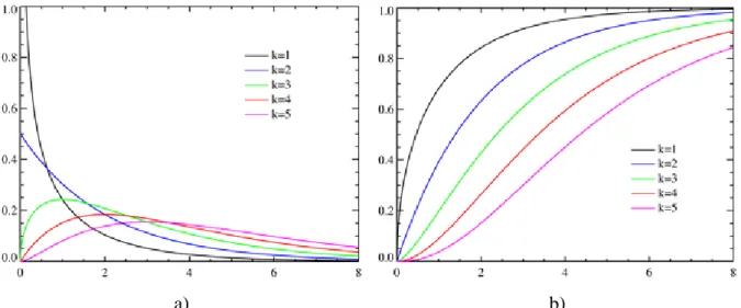
1.1 The Rayleigh distribution

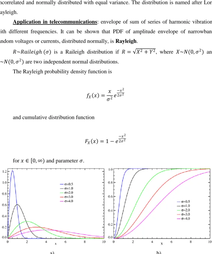
In probability theory and statistics, the Rayleigh distribution (pronounced: /'reɪlɪ/) is a continuous probability distribution. As an example of how it arises, the wind speed will have a Rayleigh distribution if the components of the two-dimensional wind velocity vector are uncorrelated and normally distributed with equal variance. The distribution is named after Lord Rayleigh.

Application in telecommunications: envelope of sum of series of harmonic vibrations with different frequencies. It can be shown that PDF of amplitude envelope of narrowband random voltages or currents, distributed normally, is Rayleigh.

𝑅~𝑅𝑎𝑖𝑙𝑒𝑖𝑔𝑕 (𝜎) is a Raileigh distribution if 𝑅 = 𝑋2+ 𝑌2, where 𝑋~𝑁(0, 𝜎2) and 𝑌~𝑁(0, 𝜎2_{) are two independent normal distributions.}

The Rayleigh probability density function is

𝑓_𝑋 𝑥 = 𝑥 𝜎2𝑒

−𝑥2 2𝜎2

and cumulative distribution function

𝐹𝑋 𝑥 = 1 − 𝑒 −𝑥2 2𝜎2 for 𝑥 ∈ 0, ∞) and parameter 𝜎.

a) b)

Properties

The raw moments are given by:

𝜇𝑘 = 𝜎𝑘2𝑘 2Γ 1 + 𝑘 2 ,

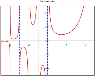
where Γ(𝑧) is the Gamma function.

In mathematics, the Gamma function (represented by the capital Greek letter Γ) is an extension of the factorial function, with its argument shifted down by 1, to real and complex numbers.

If 𝑛 is a positive integer, then Γ 𝑛 = 𝑛 − 1 ! showing the connection to the factorial function.

Figure 2: The Gamma function along part of the real axis

The mean and variance of a Rayleigh random variable may be expressed as:

𝐸 𝑋 = 𝜎 𝜋₂ ≈ 1.253𝜎,

and

The mode is 𝜎 and the maximum pdf is

𝑓_𝑚𝑎𝑥 = 𝑓 𝜎; 𝜎 =1_𝜎𝑒𝑥𝑝 −1₂ ≈0.606_𝜎 .

The skewness is given by:

𝛾1 = 2 𝜋 𝜋−3 _4−𝜋 3 2 ≈ 0.631.

The excess kurtosis is given by:

𝛾2 = −6𝜋

2_−24𝜋+16

4−𝜋 2 ≈ −0.245.

1.2 Maxwellian (Maxwell-Boltzmann) distribution

The Maxwell–Boltzmann distribution describes particle speeds in gases, where the particles do not constantly interact with each other but move freely between short collisions. It describes the probability of a particle's speed (the magnitude of its velocity vector) being near a given value as a function of the temperature of the system, the mass of the particle, and that speed value. This probability distribution is named after James Clerk Maxwell and Ludwig Boltzmann.

a) b)

Figure 3: Maxwell-Boltzmann Probability density function (a) and Cumulative distribution function (b)

Parameters: 𝑎 > 0; 𝑥 ∈ 0, ∞) . Probability density function is:

𝑓_𝑋 𝑥 = 2_𝜋𝑥2𝑒−𝑥2 2𝑎2 _𝑎3 .

Cumulative distribution function is:

𝐹𝑋 𝑥 = erf _2𝑎𝑥 − _𝜋2𝑥𝑒

−𝑥2 2𝑎2

𝑎 .

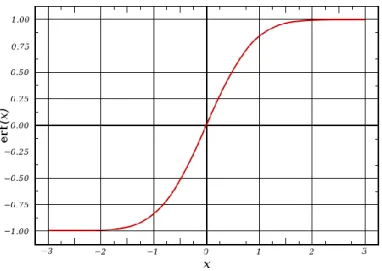
In mathematics, the error function (also called the Gauss error function) is a special function (non-elementary) of sigmoid shape which occurs in probability, statistics, materials science, and partial differential equations. It is defined as:

erf 𝑥 = 2

𝜋 𝑒 −𝑡2

𝑑𝑡

𝑥

0 .

The complementary error function, denoted erfc, is defined as

erfc 𝑥 = 1 − erf 𝑥 = 2

𝜋 𝑒

−𝑡2_𝑑𝑡 ∞

Figure 4: Error function

Numerical characteristics of Maxwellian distribution: Mean: 𝜇 = 2𝑎 2_𝜋.

Mode: 2𝑎. Variance: 𝜎2 = 𝑎

2 _3𝜋−8

𝜋 .

Skewness: 𝛾₁ =2 2 5𝜋−16 _{3𝜋−8 3 2} . Kurtosis: 𝛾₂ = −496−40𝜋+3𝜋

2

3𝜋−8 2 .

1.3 The chi-square distribution

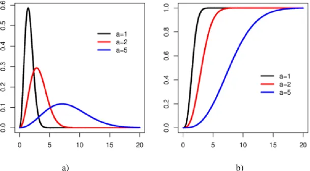
In probability theory and statistics, the chi-square distribution (also chi-squared or 𝝌𝟐 -distribution) is one of the most widely used theoretical probability distributions in inferential statistics, e.g., in statistical significance tests. A random variable is said to have a chi-square distribution if it equals the sum of the squares of a set of statistically independent standard Gaussian random variables.

a) b)

Figure 5: Chi-square Probability density function (a) and Cumulative distribution function (b)

If 𝑋₁, ..., 𝑋_𝑘 are 𝑘 independent, normally distributed random variables with mean 0 and variance 1, then the random variable 𝑄 = 𝑘_𝑖=1𝑋_𝑖2 is distributed according to the chi-square distribution with 𝑘 degrees of freedom. This is usually written 𝑄~𝜒_𝑘2.

The chi-square distribution has one parameter: 𝑘 – a positive integer that specifies the number of degrees of freedom.

In statistics, the number of degrees of freedom is the number of values in the final calculation of a statistic that are free to vary. Mathematically, degrees of freedom is the dimension of the domain of a random vector, or essentially the number of 'free' components: how many components need to be known before the vector is fully determined.

The term is most often used in the context of linear models (linear regression, analysis of variance), where certain random vectors are constrained to lie in linear subspaces, and the degrees of freedom is the dimension of the subspace. The degrees-of-freedom are also commonly associated with the squared lengths (or “Sum of Squares”) of such vectors, and the parameters of chi-squared and other distributions that arise in associated statistical testing problems.

The chi-square distribution is a special case of the gamma distribution. A probability density function of the chi-square distribution is

𝑓𝑋 𝑥; 𝑘 =

1

2𝑘 2_{Γ 𝑘 2} 𝑥 𝑘 2 −1𝑒−𝑥 2 𝑓𝑜𝑟 𝑥 > 0,

0 𝑓𝑜𝑟 𝑥 ≤ 0,

Its cumulative distribution function is:

𝐹𝑋 𝑥; 𝑘 =𝛾 𝑘 2_{Γ 𝑘 2} ,𝑥 2 = 𝑃 𝑘 2 , 𝑥 2 ,

where 𝛾(𝑘, 𝑧) is the lower incomplete Gamma function and Γ 𝑘 2 is the regularized Gamma function.

Tables of this distribution – usually in its cumulative form – are widely available and the function is included in many spreadsheets and all statistical packages.

It follows from the definition of the chi-square distribution that the sum of independent chi-square variables is also chi-square distributed. Specifically, if 𝑋𝑖 𝑖=1𝑛 are independent

chi-square variables with 𝑘𝑖 𝑖=1𝑛 degrees of freedom, respectively, then 𝑌 = 𝑋1+ ⋯ + 𝑋𝑛 is

chi-square distributed with 𝑘₁+ ⋯ + 𝑘_𝑛 degrees of freedom. Mean: 𝐸 𝑄 = 𝑘.

Median: ≈ 𝑘 −2₃+_27𝑘4 −_729𝑘8 ₂. Mode: 𝑚𝑎𝑥 𝑘 − 2, 0

Variance: 𝑉𝑎𝑟 𝑄 = 2𝑘. Skewness: 8 𝑘.

Kurtosis: 12 𝑘.

Since a Chi-2 variable is the sum of independent variables, it clearly should go to a normal distribution as the number of degrees of freedom increases.

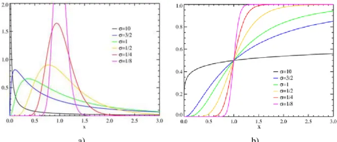
1.4 The lognormal distribution

A variable is lognormally distributed if its logarithm has a normal distribution. If 𝑌 is 𝒩(𝑚, 𝜎2_{)-distributed, then 𝑋 = 𝑒}𝑌 _{is lognormally distributed with density function:}

𝑓_𝑋 𝑥; 𝜇, 𝜎 = 1

𝜎𝑥 2𝜋𝑒

− ln 𝑥−𝜇 2 _2𝜎2

, for 𝑥 > 0,

where 𝜇 and 𝜎 are the mean and standard deviation of the variable’s natural logarithm (by definition, the variable’s logarithm is normally distributed).

Cumulative distribution function

𝐹_𝑋 𝑥; 𝜇, 𝜎 = 1₂erfc −ln 𝑥−𝜇

𝜎 2 = Φ ln 𝑥−𝜇

where erfc is the complementary error function, and Φ is the standard normal cdf.

a) b)

Figure 6: Log-normal Probability density function (a) and Cumulative distribution function (b)

The moments of the two distributions 𝑋 and 𝑌 are related. If 𝑋 is a lognormally distributed variable, its expected value (mean), variance, and standard deviation are:

𝐸 𝑋 = 𝑒𝜇 +𝜎2 2_;

𝑉𝑎𝑟 𝑋 = 𝑒𝜎2 _{− 1 𝑒}2𝜇 +𝜎2_;

s. d. 𝑋 = 𝑉𝑎𝑟 𝑋 = 𝑒𝜇 +𝜎2 2 _𝑒𝜎2 _{− 1} .

One usually proceeds the inverse way: the parameters of 𝑋 are known and one looks for the (𝑚, 𝜎) needed, e.g. to generate a sample in a simulation experiment. The correspondence is simply:

𝜎2 _{= ln 1 +}𝑉𝑎𝑟 𝑋 𝐸 𝑋 2 ;

𝜇 = ln 𝐸 𝑋 −𝜎₂2 = ln 𝐸 𝑋 −1₂ln 1 +𝑉𝑎𝑟 𝑋 _{𝐸 𝑋 2} .

Mode 𝑋 = 𝑒𝜇−𝜎2 .

The median is such a point where 𝐹𝑋 = ½:

Med 𝑋 = 𝑒𝜇_.

Skewness: 𝑒𝜎2+ 2 𝑒𝜎2− 1. Kurtosis: 𝑒4𝜎2 + 2𝑒3𝜎2 + 3𝑒2𝜎2 − 3.

The reason why the lognormal distribution is encountered is described as the principle of

multiplicative accumulation. The normal distribution appears naturally when a phenomenon results in the sum of independent perturbations. Assume now the amplitude of the phenomenon is caused by the product of independent causes. Taking the logarithm transforms the products into sums, on which the arguments of the central limit theorem apply. The lognormal distribution is thus invoked in the analysis of a large number of economic phenomena related to income or consumption, or in life sciences.

A variable might be modeled as log-normal if it can be thought of as the multiplicative product of many independent random variables each of which is positive. For example, in finance, a long-term discount factor can be derived from the product of short-term discount factors. In wireless communication, the attenuation caused by shadowing or slow fading from random objects is often assumed to be log-normally distributed.

Application in telecommunications: defining PDF of the ratio of input and output signals powers.

2 Functions of random variables

2.1Functions of discrete random variables

Consider a probability model of today’s weather, let the random variable 𝑋 be the temperature in degrees Celsius, and consider the transformation 𝑌 = 1.8𝑋 + 32, which gives the temperature in degrees Fahrenheit. In this example, 𝑌is a linear function of 𝑋, of the form

𝑌 = 𝑔(𝑋).

For example, if we wish to display temperatures on a logarithmic scale, we would want to use the function 𝑔(𝑋) = log𝑋.

If 𝑌 = 𝑔(𝑋) is a function of a random variable 𝑋, then 𝑌 is also a random variable, since it provides a numerical value for each possible outcome. This is because every outcome in the sample space defines a numerical value 𝑥for 𝑋and hence also the numerical value 𝑦 = 𝑔(𝑥) for 𝑌. If 𝑋 is discrete with PMF 𝑝_𝑋, then 𝑌 is also discrete, and its PMF 𝑝_𝑌 can be calculated using the PMF of 𝑋. In particular, to obtain 𝑝_𝑌(𝑦) for any 𝑦, we add the probabilities of all values of 𝑥 such that 𝑔(𝑥) = 𝑦:

𝑝𝑌(𝑦) = {𝑥 | 𝑔(𝑥)=𝑦}𝑝𝑋(𝑥).

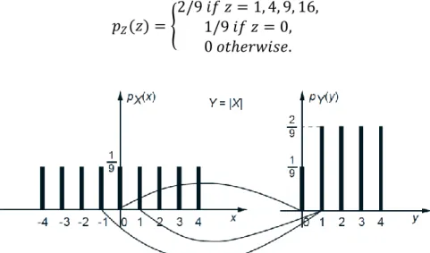
Example. Let 𝑌 = |𝑋|and let us apply the preceding formula for the PMF 𝑝𝑌 to the case

where

𝑝𝑋 𝑥 = 1/9 𝑖𝑓 𝑥 𝑖𝑠 𝑎𝑛 𝑖𝑛𝑡𝑒𝑔𝑒𝑟 𝑖𝑛 𝑡𝑕𝑒 𝑟𝑎𝑛𝑔𝑒 [−4, 4],_{0 𝑜𝑡𝑕𝑒𝑟𝑤𝑖𝑠𝑒.}

The possible values of 𝑌 are 𝑦 = 0, 1, 2, 3, 4. To compute 𝑝𝑌(𝑦) for some given value 𝑦

from this range, we must add 𝑝_𝑋 𝑥 over all values 𝑥 such that |𝑥| = 𝑦. In particular, there is only one value of 𝑋that corresponds to 𝑦 = 0, namely 𝑥 = 0.

Thus,

𝑝_𝑌(0) = 𝑝_𝑋(0) =1₉.

Also, there are two values of 𝑋that correspond to each 𝑦 = 1, 2, 3, 4, so for example,

𝑝_𝑌 1 = 𝑝_𝑋 −1 + 𝑝_𝑋(1) =2₉.

Thus, the PMF of 𝑌is

𝑝𝑌 𝑦 =

For another related example, let 𝑍 = 𝑋2. To obtain the PMF of 𝑍, we can view it either as the square of the random variable 𝑋 or as the square of the random variable 𝑌. By applying the formula 𝑝_𝑍(𝑧) = _{{𝑥 | 𝑥}2_=𝑧}𝑝_𝑋(𝑥) or the formula 𝑝_𝑍(𝑧) = _{{𝑦 | 𝑦}2_=𝑧}𝑝_𝑌 (𝑦), we obtain

𝑝_𝑍(𝑧) = 2/9 𝑖𝑓 𝑧 = 1, 4, 9, 16,1/9 𝑖𝑓 𝑧 = 0, 0 𝑜𝑡𝑕𝑒𝑟𝑤𝑖𝑠𝑒.

Figure 7: The PMFs of 𝑋and 𝑌 = |𝑋|in example.

2.2 Derived distributions

We have seen that the mean of a function 𝑌 = 𝑔(𝑋) of a continuous random variable 𝑋, can be calculated using the expected value rule

𝐸[𝑌 ] = 𝑔(𝑥)𝑓_−∞∞ 𝑋(𝑥)𝑑𝑥,

without first finding the PDF 𝑓𝑌 of 𝑌. Still, in some cases, we may be interested in an explicit

formula for 𝑓_𝑌. Then, the following two-step approach can be used.

Calculation of the PDF of a Function 𝒀 = 𝒈(𝑿) of a Continuous Random Variable 𝑿

Calculate the CDF 𝑓𝑌 of 𝑌using the formula

𝐹_𝑌(𝑦) = 𝑃 𝑔(𝑋) ≤ 𝑦 = _{{𝑥 | 𝑔(𝑥)≤𝑦}}𝑓_𝑋(𝑥)𝑑𝑥.

Differentiate to obtain the PDF of 𝑌:

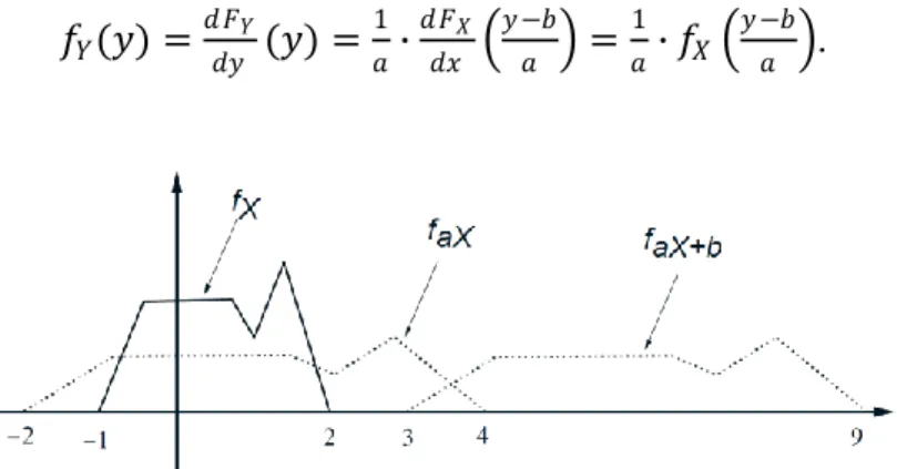
An important case arises when 𝑌 is a linear function of 𝑋. See Fig. 8 for a graphical interpretation.

The PDF of a Linear Function of a Random Variable

Let 𝑋be a continuous random variable with PDF 𝑓_𝑋, and let 𝑌 = 𝑎𝑋 + 𝑏,

for some scalars 𝑎 ≠ 0 and 𝑏. Then,

𝑓𝑌(𝑦) =_|𝑎|1 𝑓𝑋 𝑦−𝑏_𝑎 .

To verify this formula, we use the two-step procedure. We only show the steps for the case where 𝑎 > 0; the case 𝑎 < 0 is similar. We have

𝐹_𝑌(𝑦) = 𝑃(𝑌 ≤ 𝑦) = 𝑃(𝑎𝑋 + 𝑏 ≤ 𝑦) = 𝑃 𝑋 ≤𝑦−𝑏_𝑎 = 𝐹_𝑋 𝑦−𝑏_𝑎 .

We now differentiate this equality and use the chain rule, to obtain

𝑓𝑌(𝑦) =𝑑𝐹_𝑑𝑦𝑌(𝑦) =_𝑎1∙𝑑𝐹_𝑑𝑥𝑋 𝑦−𝑏_𝑎 =1_𝑎∙ 𝑓𝑋 𝑦−𝑏_𝑎 .

𝑓𝑌(𝑦) =_|𝑎|1 𝑓𝑋 𝑦−𝑏_𝑎 .

If 𝑎 were negative, the procedure would be the same except that the PDF of 𝑋would first need to be reflected around the vertical axis (“flipped”) yielding 𝑓_−𝑋. Then a horizontal and vertical scaling (by a factor of |𝑎| and 1/|𝑎|, respectively) yields the PDF of −|𝑎|𝑋 = 𝑎𝑋. Finally, a horizontal shift of 𝑏would again yield the PDF of 𝑎𝑋 + 𝑏.

The Monotonic Case

The calculation and the formula for the linear case can be generalized to the case where 𝑔 is a monotonic function. Let 𝑋 be a continuous random variable and suppose that its range is contained in a certain interval 𝐼, in the sense that 𝑓𝑋(𝑥) = 0 for 𝑥 ∉ 𝐼. We consider the random

variable 𝑌 = 𝑔(𝑋), and assume that 𝑔is strictly monotonic over the interval 𝐼. That is, either a) 𝑔(𝑥) < 𝑔(𝑥′) for all 𝑥, 𝑥′ ∈ 𝐼 satisfying 𝑥 < 𝑥′(monotonically increasing case), or b) 𝑔(𝑥) > 𝑔(𝑥′) for all 𝑥, 𝑥′ ∈ 𝐼 satisfying 𝑥 < 𝑥′(monotonically decreasing case). Furthermore, we assume that the function 𝑔 is differentiable. Its derivative will necessarily be nonnegative in the increasing case and nonpositive in the decreasing case.

An important fact is that a monotonic function can be “inverted” in the sense that there is some function 𝑕, called the inverse of 𝑔, such that for all 𝑥 ∈ 𝐼, we have 𝑦 = 𝑔(𝑥) if and only if 𝑥 = 𝑕(𝑦). For example, the inverse of the function 𝑔(𝑥) = 180/𝑥is 𝑕(𝑦) = 180/𝑦, because we have 𝑦 = 180/𝑥 if and only if 𝑥 = 180/𝑦. Other such examples of pairs of inverse functions include

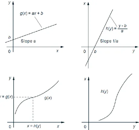
𝑔(𝑥) = 𝑎𝑥 + 𝑏, 𝑕(𝑦) =𝑦−𝑏_𝑎 ,

where 𝑎and 𝑏are scalars with 𝑎 ≠ 0 (see Fig. 9), and

𝑔(𝑥) = 𝑒𝑎𝑥_{, 𝑕(𝑦) =}ln 𝑦 𝑎 ,

Figure 9: A monotonically increasing function 𝑔(on the left) and its inverse (on the right). Note that the graph of 𝑕has the same shape as the graph of 𝑔, except that it is rotated by 90 degrees

and then reflected (this is the same as interchanging the 𝑥and 𝑦axes).

For monotonic functions 𝑔, the following is a convenient analytical formula for the PDF of the function 𝑌 = 𝑔(𝑋).

PDF Formula for a Monotonic Function of a Continuous Random Variable

Suppose that 𝑔is monotonic and that for some function 𝑕and all 𝑥in the range 𝐼of 𝑋we have

𝑦 = 𝑔(𝑥) if and only if 𝑥 = 𝑕(𝑦).

Assume that 𝑕 has first derivative (𝑑𝑕/𝑑𝑦)(𝑦). Then the PDF of 𝑌 in the region where 𝑓_𝑌(𝑦) > 0 is given by