AN ANALYSIS OF CHANGES IN STREAM TEMPERATURE DUE TO FOREST HARVEST PRACTICES USING DHSVM-RBM
A Thesis presented to
the Faculty of California Polytechnic State University San Luis Obispo
In Partial Fulfillment
of the Requirements for the Degree Master of Science in Forestry Sciences
by Julia Ridgeway
COMMITTEE MEMBERSHIP
TITLE: An analysis of changes in stream temper-ature due to forest harvest practices using DHSVM-RBM
AUTHOR: Julia Ridgeway
DATE SUBMITTED: June 2019
COMMITTEE CHAIR: Christopher Surfleet, Ph.D. Professor
Natural Resources Management and Envi-ronmental Sciences
COMMITTEE MEMBER: Bwalya Malama, Ph.D. Associate Professor
Natural Resources Management and Envi-ronmental Sciences
ABSTRACT
An analysis of changes in stream temperature due to forest harvest practices using DHSVM-RBM
Julia Ridgeway
Forest harvesting has been shown to cause various changes in water quantity and water quality parameters, highlighting the need for comprehensive forest practice rules. Studies show a myriad of impacts to ecosystems as a result of watershed level changes, such as forest harvesting. Being able to better understand the impact that forest harvesting can have on stream temperature is especially critical in locations where federally threatened or endangered fish species are located. The overall goal of this research project is to assess responses in stream temperature to various riparian and forest harvest treatments in a maritime, mountainous environment. The results of this study aim to inform decision makers with additional information pertaining to the effects of forest harvest on water temperature. Modeling is done as a part of the third Caspar Creek Paired Experimental Watershed study. Located in Mendocino County, the site provides a place for California researchers and decision makers to learn about the cumulative watershed effects of forest management operations on peak flows, sediment production, anadromous fish, macro-invertebrate communities, nutrient cycling and more.
2018-2019 SFC forest harvest and (3) an experimental design converting dominant riparian vegetation along 300-yard stream reaches.
ACKNOWLEDGMENTS
I would like to thank my graduate committee, Dr. Christopher Surfleet, Dr. Bwalaya Malama and Dr. Misgana Muleta, for their input and direction on this project; with a special note to my adviser, Dr. Surfleet, for his considerable work, guidance, support and expression of gratitude for the beautiful area that we have had the pleasure to research. Thank you to Dr. John Yearsley and Dr. Ning Sunn for their open communication and assistance with modeling questions. Thank you to the California Department of Forestry and Fire Protection (CalFire) for funding and supporting this research; the Pacific Southwest Research Station (PSW) for site specific and technical support; and the California Department of Fish and Wildlife (CDFW) for willing to share their data sets. And above all, to the many people who have tirelessly worked to maintain Caspar Creek as one of the most extensive paired watershed studies in the world, especially those with boots on the ground collecting the data that made this modeling work possible.
Finally, thank you to both the California Polytechnic State University Aerospace and Computer Sciences departments for the use of computer hardware and assistance, with a special note to Andrew Adriance for his computer programming work. To my own department, Natural Resources Management and Environmental Sciences, for supporting and inspiring me to continue on with my academic career. To Tyler Davis for his field work assistance and friendship over these past two years. And lastly, thank you to my friends and family for their undying love, support and encouragement for me to pursue my passions.
TABLE OF CONTENTS
Page
LIST OF TABLES ix
LIST OF FIGURES x
CHAPTER
1 Introduction 1
1.1 Background & Problem Statement . . . 1
1.2 Statement of Overall Research Goal . . . 2
1.3 Research Objectives . . . 2
1.4 Importance of the Project . . . 2
1.5 General Approach . . . 3
1.6 Scope . . . 4
1.6.1 Location . . . 4
1.6.2 Date and Timing . . . 4
1.6.3 Equipment . . . 4
2 Literature Review 6 2.1 Introduction . . . 6
2.2 Evolution of the California Forest Practice Rules . . . 6
2.2.1 Watercourse and Lake Protection Zones (WLPZ) . . . 11
2.3 Water Temperature . . . 13
2.3.1 Importance . . . 14
2.3.2 Impacts from Forest Harvesting . . . 17
2.4 Hydrologic Modeling . . . 21
2.4.1 DHSVM . . . 22
2.5 Stream Temperature Modeling . . . 25
2.5.1 RBM . . . 27
2.6 Caspar Creek Paired Experimental Watershed . . . 32
2.6.1 History . . . 32
3.2 DHSVM Background . . . 39
3.2.1 DHSVM Inputs . . . 39
3.3 RBM Background . . . 44
3.3.1 RBM Inputs . . . 45
3.4 Model Calibration . . . 53
3.4.1 RBM . . . 53
3.4.2 DHSVM . . . 54
3.5 Modeling Scenarios . . . 55
3.5.1 Canopy Reduction . . . 56
3.5.2 SFC Phase Three Harvest Scenario . . . 57
3.5.3 Riparian Vegetation Conversion . . . 59
3.6 Sensitivity Analysis . . . 61
4 Results 63 4.1 DHSVM . . . 63
4.2 RBM . . . 65
4.3 Modeling Scenarios . . . 68
4.3.1 Canopy Reduction . . . 68
4.3.2 SFC Phase Three Harvest Scenario . . . 72
4.3.3 Riparian Vegetation Conversion . . . 73
4.4 Sensitivity Analysis . . . 74
5 Discussion 80 5.1 RBM Calibration . . . 80
5.2 Modeling Scenarios . . . 82
5.2.1 Canopy Reduction . . . 82
5.2.2 SFC Phase Three Harvest Scenario . . . 83
5.2.3 Riparian Vegetation Conversion . . . 85
5.3 Sensitivity Analysis . . . 85
5.4 Limitations and Future Work . . . 87
6 Conclusion 88
BIBLIOGRAPHY 91
LIST OF TABLES
Table Page
2.1 WLPZ Widths . . . 12
2.2 WLPZ Zone Widths . . . 12
2.3 Maximum Fish Temperature Tolerances . . . 16
3.1 Physical Characteristics of SFC Sub-Watersheds . . . 37
3.2 Cloud Cover Values . . . 43
3.3 Mohseni Parameters . . . 48
3.4 Leopold Parameters . . . 51
3.5 Initial Riparian Characteristics . . . 52
3.6 DHSVM Variables . . . 55
3.7 Canopy Reduction Riparian Characteristics . . . 57
3.8 Sub-Watershed Harvest Scenario LAI Values . . . 58
3.9 Sensitivity Analysis Parameters . . . 62
4.1 DHSVM Statistical Fit . . . 63
4.2 MWAT Results . . . 68
LIST OF FIGURES
Figure Page
2.1 Timeline of Forest Practice Rules . . . 10
2.2 Example WLPZ . . . 11
2.3 Effects of Forest Practices on Hydrologic Processes . . . 18
2.4 Model Representation of DHSVM . . . 23
3.1 SFC Map . . . 38
3.2 SFC Road Locations Map . . . 39
3.3 South Fork Caspar Creek Meteorological Station . . . 41
3.4 RBM Riparian Shading . . . 45
3.5 Development of Mohseni Parameters - Outliers Included . . . 47
3.6 Development of Mohseni Parameters - Outliers Excluded . . . 48
3.7 Leopold Parameters - Cross Section . . . 50
3.8 Leopold Parameters - Relationships . . . 51
3.9 Harvest Map . . . 59
3.10 Riparian Vegetation Conversion Map . . . 60
3.11 Blithe, CA Comparison Map . . . 61
4.1 DHSVM Calibration . . . 64
4.2 RBM Calibration . . . 67
4.3 Canopy Reduction - Class I Streams Only . . . 69
4.4 Canopy Reduction - All Stream Classes . . . 71
4.5 Canopy Reduction - Change in Temperature . . . 72
4.6 Harvest Scenario . . . 73
4.7 Riparian Vegetation Conversion . . . 74
4.8 Sensitivity Analysis - Riparian Vegetation Characteristics . . . 75
4.9 Sensitivity Analysis - Air Temperature and Relative Humidity . . . . 77
Chapter 1
Introduction
1.1 Background & Problem Statement
The California Forest Practice Rules (FPR) attempt to mitigate the impacts that forest harvesting can have on forested ecosystems. This study aims to link policy to environmental outcome, by examining stream temperature responses to various components of the most up-to-date California FPRs.
1.2 Statement of Overall Research Goal
The overall research goal of this project is to better understand the impacts that changes in riparian shading and forest harvest have on stream temperature in a coastal watershed.
1.3 Research Objectives
• Calibrate the Distributed Hydrology Soil Vegetation Model (DHSVM) and the
River Basin Model (RBM) to measurements of flow and stream temperature in the South Fork Caspar Creek (SFC).
• Determine the impact of the size and structure of California Forest Practice
Rules “Watercourse and Lake Protection Zones (WLPZs)” on stream tempera-tures.
• Determine the impact of a modern forest harvest scenario on stream
tempera-ture.
• Determine the impact of a theoretical riparian vegetation conversion on stream
temperature.
1.4 Importance of the Project
harvesting can have on stream temperatures is essential to protecting the habitat for aquatic species that are sensitive to changes.
Caspar Creek is home to endangered and threatened Coho Salmon(Oncorhynchus kisutch) and Steelhead trout (Oncorhynchus mykiss). Low flows occurring during peak summer temperatures have the potential to create additional stress and delete-rious habitat for salmonid species. California FPRs have been put in place to attempt to mitigate impacts such as these. However it is important to link policy to environ-mental outcome. Therefore, the results of this study aim to provide policy makers additional information to create conscientious, feasible regulations.
1.5 General Approach
1.6 Scope
1.6.1 Location
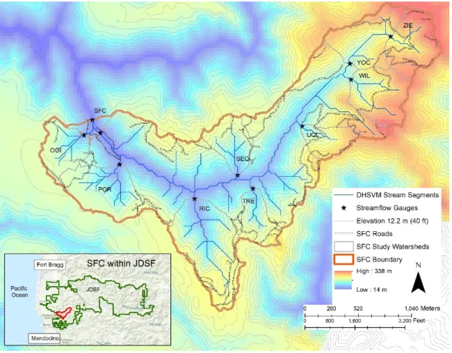
The study area evaluated was the South Fork within the Caspar Creek Experimen-tal Watershed, located on the Jackson Demonstration State Forest near Fort Bragg, California (Figure 3.1 and 3.2). The research watershed is located in the northern part of the California Coast Ranges and has a total area of 2,167 ha. A detailed description of the study site is located in the Caspar Creek overview (Section 2.6) of this report.
1.6.2 Date and Timing
Data collection has been on going in Caspar Creek since its establishment in 1961. This study will focus only on the South Fork of Caspar Creek using data collected between 2009 and 2016; specially analysis of stream temperatures was for the 2011-2016 hydrologic years. The majority of data used in this study came from the experimental watershed itself. However, for those variables not collected on site, or to fill gaps in Caspar collected datasets, other sources included the California Irrigation Management Information System (CIMIS), a Meso-West meteorological station and the National Centers for Environmental Information (NCEI) Arcata Airport station.
1.6.3 Equipment
Chapter 2
Literature Review
2.1 Introduction
This literature review focuses on elements related to California Forest Practice Rules (FPR), the importance of stream temperature in forest environments, the effect that forest harvesting has on stream temperature, hydrologic and stream temperature computer modeling, the Distributed Hydrology Soil Vegetation Model (DHSVM), the River Basin Model (RBM) and the Caspar Creek Paired Experimental Watershed Study.
2.2 Evolution of the California Forest Practice Rules
with the gold rush, (2) susceptibility of California to wildfire due to climate, (3) advanced perception that vegetative cover could aid in watershed protection and (4) the conventional idea of reforesting harvested areas and afforesting treeless brush and grasslands to create more timber (Clar, 1957). Some early efforts to manage pest outbreaks took place, and the creation of work camps to address high unemployment rates from the Great Depression started to spur legislation. However, overall the primary focus of legislation was on fire prevention and slash disposal (Arvola, 1976). In 1927 the Legislature created the Department of Natural Resources (Chapter 128) four divisions: forestry, mines and mining, parks, and fish and game (Clar, 1957). In 1943 Governor Earl Warren signed into act Chapter 172 of the 1943 Legislative Session, the “minimum-diameter law”, which was essentially the first step to what would become the California Forest Practice Act (Arvola, 1976; Clar, 1957). These statutes also established a legislative Forestry Study Committee, who developed an extensive proposal for forestry legislation that were accepted in 1945. Again, initially these rules were focused on fire protection and reforestation.
In 1998 the state agreed to organize an independent panel of scientists to com-plete a comprehensive review of the FPRs ability to protect salmonid species. A formal report by Ligon et al. (1999) was completed, concluding that the FPRs were not protecting salmon and Steelhead populations from cumulative watershed effects, both temporally and spatially. Recommendations were to improve enforcement and regulations regarding on-site operations and road maintenance, that would reduce sediment production, improve stream habitat and guarantee unrestricted passage for migration.
Studies during the early 2000’s continued with this movement, highlighting a need to review the impact of forest practices on water quality. These reports ultimately concluded that the THP method was insufficient at: addressing effects on watersheds, due to being too subjective at accessing current resource conditions and the poten-tial for additional impacts (The Univeristy of California Committee on Cumulative Watershed Effects, 2001); protecting water quality and endangered species (Kersten, 2002); or allowing enough time for review and estimation of the risk and resources associated with proper examination (Humboldt Watersheds Independent Scientific Review Pannel, 2003). Subsequently, the state published the Recovery Strategy for California Coho Salmon, which required a forest practice monitoring group be set up. Since then, the Board of Forestry has worked to improve riparian areas through the implementation of Watercourse and Lake Protection Zones (WLPZs) and other impact mitigation measures.
2.2.1 Watercourse and Lake Protection Zones (WLPZ)
Buffer strips, also referred to as Watercourse and Lake Protection Zones (WLPZs), first began to be required along fish bearing streams in California in 1973 (Caffer-ata, 1990). CalFire states that the two primary functions of WLPZs are to provide shade for water temperature and longterm inputs for large woody debris. Additional functions include filtering inputs of fine sediments, maintenance of microclimates for temperature and humidity, and the input of energy in the form of organic debris that supports other biota (Ligon et al., 1999).
Figure 2.2: Example WLPZ. WLPZ buffer from the NFC study (IVE tributary lower left, MUN upper right). Figure excerpted from Cafferata and Reid (2013); taken in March 1990.
Table 2.1: WLPZ Widths. WLPZ width based on stream class and slope (Cal-ifornia Department of Forestry and Fire Protection, 2019). “Discretionary” defers decisions to the Registered Professional Foresters (RPFs) or CalFire.
Stream Class <30% Slope 30-50% Slope >50% Slope
Class I 75’ 100’ 150’
Class II 50’ 75’ 100’
Class III Discretionary Discretionary Discretionary
Class IV N/A N/A N/A
For areas where anadromous fish are present, California uses a three zone setup within WLPZs. The core zone is meant to promote bank stability, wood recruitment by bank erosion and canopy retention. Therefore no harvesting is allowed in this zone. The inner zone has a no-harvest prescription and the primary objective is to provide large wood, shading and ecological diversity. Lastly, logging is allowed in the outer zone, which is meant to protect the inner two zones, such as for wind protection and microclimate control. The size of the three zones are based on geographic location and are outlined in Table 2.2.
Table 2.2: WLPZ Zone Widths. Width of each zone within a WLPZ, based on geographic location of the stream (California Department of Forestry and Fire Protection, 2019).
Geographic Location WLPZ Width Core Inner Outer
Non-anadromy zone 100’ 30’ 40’ 30’
Anadromous Fish Present 150’ 30’ 70’ 50’
Flood prone area 150-200+’ 30’ A:70-120’B: End of FA End of FA+50’
Additional rules for areas with anadromous fish by each stream class include:
• Class I streams: Post-harvest canopy must be composed of both conifer and
the 13 largest trees per acre (TPA) must be kept. Forest harvest operations are allowed in the outer zone as long as 50% of the overstory canopy cover is retained.
• Class II streams: the inner zone requires 60% overstory canopy retention and
has as a TPA requirement of 7. The outer zone requires 50% retention of the overstory canopy cover.
• Class III and IV streams: there is no distinction of core, inner and outer zones.
However, a 20 foot buffer along streams with slopes >30% and a 30 foot buffer
along streams with slopes<30% , where all trees must be retained, is required.
Trees that fall outside of these buffers are subject to “normal” harvesting prac-tices.
2.3 Water Temperature
Like with the environmental awakening that lead to the creation of the FPRs, public awareness of anthropogenic degradation in rivers and streams increased during the 1970’s. Since then, water temperature has been regulated across the United States by the Federal Water Pollution Control Act, also known as the Clean Water Act, in Sections 316a and 316b. For California, the State Water Board set up nine Regional Water Quality Control Boards to address localized differences in climate, topography, geology and hydrology. Water quality standards are set by regional Basin Plans, as well as statewide Plans and Policies. In cold water systems, like Caspar Creek, the primary regulation overseeing stream temperature protection is that:
Processes that may raise stream temperatures can be broken down into “first”, “second” and “third-order” controls, as described by Dugdale et al. (2017). First order controls include climatic and hydrological processes that dictate headwater temperatures and control rates of downstream warming or cooling due to radiative, latent (evaporation), sensible and advective (groundwater, hyporpheic and transient storage) heat exchanges. Second and third order controls are those that alter the degree to which first order processes can affect stream temperature. Second order controls occur at the whole-river scale, such as riparian forests and steep topography, while third order controls act on the reach scale, such as channel morphology and topology. Dugdale et al. (2017) acknowledges that although the effect of individual processes on stream temperature have been well studied, the way they amalgamate with one another is still being researched.
Literature reviews pertaining to all aspects of stream temperatures include Smith (1972), Ward (1985), Caissie (2006) and Webb et al. (2008). This literature review will focus only on the importance of stream temperature in regards to fish species, as well as studies analyzing the impacts of forest harvest on stream temperature, spotlighting those from the Pacific Northwest.
2.3.1 Importance
pro-duction of energy (Strzepek et al., 2015). Yet most often, scientists and management officials are concerned with the lethal stress water temperatures can have on cold water species, such as mayflies, stoneflies and certain fish species (Quinn et al., 1994; Eliason et al., 2011). For this reason, and that Caspar Creek is home to threatened Steelhead trout(Oncorhynchus mykiss)and endangered Coho Salmon(Oncorhynchus kisutch), this section will primarily focus on the importance stream temperature plays in regards to fish.
Freshwater fish species are of particular concern due to their importance as indica-tors of ecosystem health and shrinking populations. Fish are poikilotherms, meaning that their body temperature directly relates to the external environment that they live in, giving them little control over body temperature. As a result, metabolism is greatly affected by water temperature and thus the need for food increases with water temperature. If food is available and dissolved oxygen is sufficient a fish will grow. However, if food is limited or other stresses exist (low dissolved oxygen, pollution, etc.) then the fish will not grow to its potential, within physiological limits. With higher stream temperatures, oxygen demand will increase in fish species while there is decreased dissolved oxygen. Therefore, different seasons, weather and time of day cause oxygen concentrations to change. It has been suggested that growth stops when water temperatures exceed 18 to 20.3°C (Welsh et al., 2004; Armour, 1991). Beyond such limits, even if food is available water temperature can be stressful enough to become lethal to the fish (Ligon et al., 1999).
temperature are cumulative and positively correlated to the duration and severity of the exposure (Ligon et al., 1999).
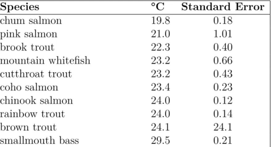
Eaton et al. (1995) determined the estimated maximum stream temperature tol-erances using field surveys for various fish species (Table 2.3). For Coho salmon, they was also reported that alternate literature found the maximum growth tolerance to be 15°C and the EPA (1976) water quality criteria for growth and survival was between 18 and 24°C. Other studies reported that physiological stress and blockages to migration for Coho salmon occur from 19 to 23°C, and 21 to 24°C for Steelhead trout (McCullough et al., 2001). The lower range of annual maximum stream temper-ature was 22.3°C for Steelhead presence in a study conducted in southern California (Sloat and Osterback, 2013). On the Mattole River, just north of Caspar Creek, juvenile Coho were not present in streams where the Maximum Weekly Average Tem-perature (MWAT) exceeded 16.7°C or the Maximum Weekly Maximum TemTem-perature (MWMT) exceeded 18.0°C (Welsh et al., 2004). Differences in these studies point to the wide discrepancy in determining a single value to protect fish species.
Table 2.3: Maximum Fish Temperature Tolerances. 95th percentile weekly mean temperatures for the highest 5% of Fish/Temperature pairs based on temporal and spatial field data (Eaton et al., 1995).
Species °C Standard Error
chum salmon 19.8 0.18
pink salmon 21.0 1.01
brook trout 22.3 0.40
mountain whitefish 23.2 0.66
cutthroat trout 23.2 0.43
coho salmon 23.4 0.23
chinook salmon 24.0 0.12
rainbow trout 24.0 0.14
brown trout 24.1 24.1
Potential increases in water temperature as a result of land cover change, water management and/or climate change pose a threat to biodiversity and aquatic ecosys-tems (Hester and Doyle, 2011). Studies have shown an increase in water temperatures throughout North America and Europe as a result of water diversion for irrigation and water supply, water confinement, thermal discharge and land use change such as logging, farming and urbanization (Kaushal et al., 2010; Foreman et al., 2001; Morrison et al., 2002; Webb and Nobilis, 1995, 2007). A 2018 Intergovernmental Panel on Climate Change Report, states that increases in mean air temperatures and the probability of drought, precipitation deficits and extreme low flow events in the Western United States should be expected, all of which would negatively impact the availability of cold freshwater (Hoegh-Guldber et al., 2018). Furthermore, it has been shown that climate change is likely to exacerbate these issues and further increase water temperature (Van Vliet et al., 2011; Meyer et al., 1999) or be magnified when paired with changes in hydrologic regimes (Mantua et al., 2010).
A major issue with truly understanding the effect of water temperature on fish species is due to the symbiotic nature between factors such as food availability, previ-ous exposure to stress, genetic adaptation, age and size (Ligon et al., 1999). Eliason et al. (2011) suggests the use of site-specific approaches to determine appropriate thermal regulations for different streams, because of cardio-respiratory physiology differences at the population levels in Fraser River sockeye salmon. Better under-standing the impacts that forest harvesting can have on water temperatures, will aid in conservation approaches that aim to protect these and other freshwater organisms.
2.3.2 Impacts from Forest Harvesting
(Buttle, 2011). However, because the primary concern for forest management in California was initially fire protection, little effort was given to watershed projects during the late 1800’s and early 1900’s (Clar, 1957). Since then, various studies have been completed to analyze the impacts of forest harvesting on hydrology for forests in California (Keppeler and Ziemer, 1990; Klein et al., 2012; Cafferata and Reid, 2013; Jones et al., 2013). Although forest management techniques can affect watershed hydrology in a plethora of ways (Figure 2.3), this review will only focus on the effects forest harvesting has on stream temperature for studies specifically done in the Pacific Northwest area.
Even with decades of research throughout the Pacific Northwest, there is still much debate regarding the thermal impact of forest harvesting (Moore et al., 2005). It is commonly accepted that the removal of shade canopy increases stream temper-atures (Carroll et al., 2004; Lynch and Corbett, 1990; Patric, 1980; Wilkerson et al., 2006; Johnson and Jones, 2000; Moore et al., 2005; Beschta et al., 1987; Brown and Krygier, 1970) and the general consensus in temperate, rain-dominated ecosystems, is that harvesting without incorporating a riparian buffer significantly increases sum-mer water temperatures, especially maximum values and diurnal range (Moore et al., 2005).
Studies to evaluate how changes in water temperature persist downstream are one such phenomenon under debate in regards to forest harvest effects on stream temperatures. Story et al. (2003) studied two reaches and found that for one stream, cooling did not occur until downstream groundwater inflows were introduced (150 m). However at a second reach, temperatures were more stable because of continuous groundwater inputs. These results spotlight the influence of hydrology on temperature patterns.
For example, Sweeney and Newbold (2014) conducted a review of the effectiveness of streamside forest buffers on various factors. Concluding that, for temperatures, buffer widths greater than or equal to 20 m keep stream temperatures within 2°C, compared to a fully forested watershed. Additionally concluding that full protection from measurable temperature increases can only be assured by a buffer width of greater than or equal to 30 m. On the other hand, Gomi et al. (2006) concluded that 30 m buffers were effective at minimizing post-harvest stream warming, but added that the 10 m buffer also appeared to minimize warming but with confounding results due to short-term data collection. A study done in British Columbia however recorded increases of 4-6°C five years following harvest, regardless of using 20 or 30 m buffers.
Orientation of the stream (E-W vs N-S) is also widely recognized as playing an important role in the effectiveness of riparian buffers (Gomi et al., 2006; Larson and Larson, 1996; DeWalle, 2010). Gomi et al. (2006) found that streams exhibiting a N-S orientation are well shaded from late morning to early afternoon, even at only a 10 m width. DeWalle (2010) found that for E-W streams, no additional shading was provided by buffers larger than 6-7 m, whereas for N-S streams optimum buffers were approximately 18-20 m, although notably less defined. However, it is noted that wider buffers may be sought to provide for benefits other than shade.
2.4 Hydrologic Modeling
Various types of hydrologic models exist, which can be broken down by two clas-sification systems. First, hydrolgic models can be either deterministic or stochastic (Dwarakish and Ganasri, 2015). Deterministic models are physically based, run by parameters in equations that predict physical processes. Stochastic models are at least partially random, using probability distributions to make predictions. From there, deterministic models can either be lumped, semi-distributed or distributed. Lumped models use spatially averaged characteristics and are generally applied to a specific point. Semi-distributed models divide the watershed into units based on vari-ables such as land cover, soil type or slope. Lastly, distributed models use a gridded format, defining model variables as functions of spacial dimensions.
Additionally, hydrologic models have been developed based on their hydrological processes, classifying them as conceptual, empirical or fully physical models. Em-pirical models build relationships between input and output on hydro-meteorological data, but are limited in that they do not consider physical processes such as sub-surface flow and infiltration. Conceptual models simplify complex processes, with portions of the model described by empirical functions based on observations. Lastly, fully physical models use only physical equations to explicitly represent the spatial variability of land surface characteristics and climatic parameters.
to study various topics including drought (Cayan et al., 2010), flooding (Das et al., 2011), declining snowpacks (Mote et al., 2005), climate change (Beyene et al., 2010) and hydropower (Christensen et al., 2004). However, because VIC simulations are intended for larger scale use, having shown fine-scale biases that become less impor-tant at broader scales (Yearsley, 2012; Wenger et al., 2010), DHSVM was used for this study. Additional factors in decision making included previous user history and that Wenger et al. (2010) noted VIC had particular difficulty in predicting summer high and low flows, which was the primary goal of the stream temperature modeling.
2.4.1 DHSVM
DHSVM-RBM numerically represents, with high spatial resolution, the effects of local weather, topography, soil type, and vegetation on hydrologic processes within watersheds. The model was developed in the early 1990’s (Wigmosta et al., 1994) and then worked on at the Pacific Northwest National Laboratory (PNNL) and the University of Washington by a variety of people under the direction of Dennis P. Lettenmaier. Since then, the model has been evaluated to be a successful tool in simulating various different forested watersheds (Whitaker et al., 2003; Thyer et al., 2004), hydrologic changes relating to climate change (Elsner et al., 2010; Brennan, 2015), glacial recession (Naz et al., 2014), forest harvesting (Storck et al., 1998; Kura et al., 2012), fire (Stonesifer, 2007; Surfleet et al., 2014), and roads (Surfleet et al., 2011; La Marche and Lettenmaier, 2001; Bowling and Lettenmaier, 2001).
distribu-tion of soil moisture, snow, evapotranspiradistribu-tion, and runoff in hourly or longer time increments for individual grid cells, or pixels, based on the digital elevation model of the watershed. Meteorological inputs required for each time increment of the model are precipitation, relative humidity, air temperature, wind speed, shortwave radia-tion and longwave radiaradia-tion. A one-dimensional water balance is calculated for each grid point based on effects from vegetation, climate, soil hydraulic properties and topography. The model uses a two layer canopy representation to calculate intercep-tion and evapotranspiraintercep-tion of vegetaintercep-tion, a two-layer energy balance model for snow accumulation and snowmelt, a multilayer unsaturated soil model based on Darcy’s Law and a saturated subsurface flow model. Once the water balance calculations are complete, each grid cell exchanges water with adjacent grid cells, which results in a three-dimensional redistribution of surface and subsurface water across the water-shed. Streamflow in channel segments is generated by channel interception of surface and sub-surface flows in the grid cell it is located (Wigmosta and Perkins, 2001).
Storck et al. (1998) applied DHSVM to assess the hydrologic effects of forest har-vesting in the Pacific Northwest for three different scenarios. For rain-on-snow events they estimated a 31% and 10% increase in peak runoff between mature vegetation and a clearcut scenario for two separate years. For spring snowmelt they estimated only a 3% decrease in peak spring streamflow events if mature vegetation was used, compared to current vegetation, and up to a 30% increase if a maximum possible harvest vegetation was simulated. Lastly, utilizing DHSVM’s road runoff algorithm showed increases in peak runoff of around 16% for the five largest events.
Bowling et al. (2000) also used DHSVM to study the effects of logging in the Wash-ington area, finding that trends were dominated by climate fluctuations. Looking at catchment pair differences, they found that peak flow changes increased following treatments, but decreased with an increasing return interval of about 10-years. How-ever, because of the small number of catchment pairs available to study, they could not reach a definitive conclusion. Using a second, alternative approach they also detected increasing trends in the peak flow series.
2.5 Stream Temperature Modeling
Section 316 of the Clean Water Act specifically identifies thermal discharge as a pollutant, creating a need for models that estimate potential impacts with changes to land use/land cover and climate. Earliest research for stream temperature stud-ies used simplistic relationships between air temperature and elevation (Walker and Lawson, 1977; Stefan and Preud’homme, 1993). Today, various stream temperature models exist for a variety of spatial and temporal resolutions.
Stream temperature models can be divided into two major types: physics based (sometimes refereed to as ‘deterministic’, ‘mechanistic’ or ‘process based’) and sta-tistical. Physical models are built on mathematical equations governing physical processes, whereas statistical models rely heavily on air temperature data inputs cou-pled with statistical relationships. Statistical models, such as those used by Risley et al. (2003), Mohseni et al. (1998) and Donato (2002), are best used in large scale op-erations, where high data requirements make physical models impractical. However, statistical models are limited in that they cannot determine specific energy transfer mechanisms responsible for stream temperature patterns (Dugdale et al., 2017) and they use past information, therefore limiting the ability to predict future impacts if variables changed. Given that DHSVM-RBM is a physically based stream tempera-ture model, the majority of this review focuses on these types of models. Benyahya et al. (2007) provides a detailed review of statistical water temperature models, if needed.
geometry, land use and hydrology to simulate land use change, altered hydrologic regimes, introduction of water impoundment structures and projected climate change. They are useful in providing process-based insights to drivers of stream temperature, information for metrics to use in larger statistical models and for forecasting tem-perature responses to scenarios where statistical models may not be usable (Dugdale et al., 2017). One-dimensional physically based models simulate rivers and stream that are well-mixed, whereas for more complex environments (those that include lakes and estuaries) models may require the use of higher order dimensions.
Heat exchanges (additions and losses of heat to the river) occur in two locations within a natural river system: the air-water interface and the streambed-water in-terface. Additional fluxes can also occur if thermal effluent and water extractions are occurring on a river system. Solar radiation, net long-wave radiation, evapora-tion and convective heat transfer affect the air-water interface. Geothermal heating through conduction, advection from groundwater and hyporheic flows are the primary functions that affect the streambed-water interface (Caissie, 2006). Heat inputs to a river system include incoming short and long-wave radiation, condensation, chemical and biological processes and friction with the streambed and streambanks. Losses in-clude reflected solar radiation and evaporation, while transfers occur through channel discharge, hyporheic exchanges, groundwater up and down-welling, tributary inflows and precipitation (Hannah and Garner, 2015).
Other physically based temperature models include the Reduced Parameter Stream Temperature Model (Cheng and Wiley, 2016) and that developed by Roth et al. (2010), which uses a one-dimensional temperature model coupled with distributed temperature sensing technology.
2.5.1 RBM
The River Basin Model (RBM) is a one-dimensional stream-temperature model that solves time-dependent equations for the conservation of thermal energy in a moving stream using a mixed Eulerian-Lagrangian, or semi-Lagrangian, numerical scheme (Yearsley, 2009). Eularian models calculate change in water temperature as a function of time (t) and use a reference system that is fixed in space through which water flows (Eq. 2.1). Lagrangian models calculate the difference in water temperature as a function of space using a reference system that moves with the water (Eq. 2.2) (Hannah and Garner, 2015).
dTw
dt =
Qn(i,t)
ρCD(i,t)
(2.1)
dTw
dx =
W(i)[Qn(i,t)] C∗F(i,t)
(2.2) Where, ρis the density of water,D is the river depth,C is the specific heat capacity
of water, Qn is the total energy available to heat or cool the water, W is the width of the stream surface and F is the river discharge.
RBM uses stream depth and an effective reach speed to solve one-dimensional, time-dependent thermal energy budget equations. It assumes that an exchange of energy across the air-water interface and advected energy from tributaries and point sources capture the important changes in rivers dominated by advection (Yearsley, 2012). The disaggregated meteorological forcing files supplied by the hydrologic sim-ulations, in our case DHSVM, provide the data required to estimate the flux of ther-mal energy at the air-water interface for each grid cell (Yearsley, 2012). Output from RBM includes hydraulic parameters, stream speed and thermal energy fluxes at the air-water interface (per grid cell).
DHSVM-RBM calculates direct solar radiation received at the stream surface through calculating the attenuation of the solar ‘beam’ as it travels through the tree canopy. Then, the fraction of the diffuse radiation received by the stream is quantified separately, by means of an algorithm that computes the reach’s sky view factor, a coefficient that represents the fraction of the hemisphere that is unblocked by tree cover/topography. DHSVM-RBM also applies shading correction to longwave fluxes. This setup is depicted in Figure 3.4, included later in the report.
Like the majority of other stream temperature models, DHSVM-RBM computes evaporation rates using Dalton’s equation, wind speed, actual vapour pressure and saturation vapour pressure. Similarly, DHSVM-RBM also incorporates bed heat fluxes into the energy balance computation. DHSVM-RBM is unique in that the hydrologic model component allows for computation of groundwater inflows and the Lagrangian structure allows inflow from different courses (tributaries and groundwa-ter) at each cell (Dugdale et al., 2017).
zero mean and that the differences between the nominal solutions and the true states are small enough that terms higher than first-order in the Taylor series expansion can be neglected (Yearsley, 2012). RBM solves the thermal energy budget equation with a semi-Lagrangian numerical method to simulate nominal water temperatures by tracking individual water parcels along their flow characteristics and storing the simulated results at discrete points on a fixed grid (Yearsley, 2009).The initial head-water conditions of RBM are estimated using the Mohseni et al. (1998) nonlinear regression model or estimates of soil temperature.
Manson et al. (2001) demonstrated that Semi-Lagrangian methods are scalable in space and time and are stable and accurate at large time steps in numerical solutions of transport when advection dominates. The change in water temperature for the particle during a time step is estimated using the speed of the particle, water depth, net exchange across the air-water interface (energy budget) and advected heat sources (tributary inputs). The model assumes that the water body is well mixed vertically and laterally, meaning density effects due to temperature gradients are neglected. Because of this, the temperature model can be uncoupled from the model simulating flow velocity and water depth, meaning these values can be simulated with other models (Yearsley, 2009). Sinokrot and Stefan (1994) concluded that although the flux of thermal energy from the stream bottom is a surface-area related phenomenon, it is generally small and can be assumed negligible.
sys-assessment of how well the methods of RBM are able to simulate water temperatures when sharp fronts associate with rapid changes in flow and temperature occurred. The study demonstrated the assumption that neglecting the dispersion of the front when simulating water temperature is reasonable.
The second river system tested, the Columbia River, was used to demonstrate applications to large-scale questions as a preliminary analysis of the impact of climate change on water temperatures. The Columbia River Basin has a drainage area of more than 670,800 km2 and is located in British Columbia, Canada and parts of Idaho, Oregon, Washington and Wyoming. The system has an annual average stream flow of 6,540 m3/second recorded at the mouth. The upstream river system has been highly developed by dams and reservoirs, causing many segments of the river to exceed water temperature criteria protecting cold water species (Yearsley, 2001).
In the case of the Columbia and Snake river simulations, differences between predicted and measured values were said to be due primarily to what can be char-acterized as parameter estimation, rather than to the inaccuracies in the numerical scheme. Uncertainty in parameter estimation include weather data from distant loca-tions used to characterize heat fluxes, estimating hydraulic variables using simplified stream hydrodynamics and uncertainty in the formulation of energy budget terms (Yearsley, 2009).
during summer periods; that basin-wide land cover and riparian vegetation have minor effects of stream temperatures during winter high flows; and that the effects of riparian vegetation during summer months is comparable to that of climate change.
Other studies using RBM thus far have included:
• Perry et al. (2011) used RBM to address potential impacts to water
tempera-tures following dam removal under various climate change scenarios.
• Van Vliet et al. (2012a) adapted RBM to be used at large spatial and temporal
scales, then applying it to a variety of different questions, including: the effect of climate change on global river flows and water temperatures (Van Vliet et al., 2013, 2015); impacts of drought and climate change on water resources and electricity supply (Van Vliet et al., 2016; Vliet et al., 2013); and the impacts of cooling water use in the energy sector (Van Vliet, 2012; Van Vliet et al., 2012b).
• Brennan (2015) compared RBM to Ficklin and Barnhart (2014)’s SWAT and
Mohseni et al. (1998)’s Nonlinear Regression model, rating VIC-RBM the high-est in performance.
• Raptis et al. (2016) and Raptis and Pfister (2016) looked at worldwide thermal
pollution patterns and power-related freshwater thermal emissions.
• Dugdale et al. (2017) reviewed various process-based models, outlining some the
similarities and differences between DHSVM-RBM and other water temperature models.
• Tobin et al. (2018) evaluated the vulnerability and resilience of various
• Niemeyer et al. (2018) integrated RBM with a two-layer stratified reservoir
mod-ule in order to account for the effects of reservoir stratification on downstream water temperatures.
• Truitt (2018) studied the effects of climate change on the Nooksack River basin.
2.6 Caspar Creek Paired Experimental Watershed
Paired watershed studies allow scientists to evaluate components of ecosystems, while essentially holding meteorological factors in an area constant. Effectiveness studies using paired watersheds in the Western United States include: the Alsea and Trask River Watersheds in the Oregon Coast Range, Hinkle Creek in the Oregon Cascades, Mica Creek Experimental Watershed in northern Idaho and the Caspar Creek Paired Experimental Watershed Study in Mendocino, California.
2.6.1 History
Napolitano et al. (1989) discussed the history of logging in Caspar Creek, which began in 1860 by business partners William H. Kelly and William T. Rundle. The duo purchased 5,000 acres and built a sawmill at the mouth of the creek. Four years later the company was taken over by Jacob Green Jackson, who had three crib dams built on the North, South and main stems of Caspar Creek for log driving operations. Concurrently, skid roads built as straight and level as possible for oxen, and later bulls, were built to transport cut logs. In these early days, burning of slash in the late summer or early fall was done to ease skidding along sloped roads (Sullenberger, 1980). The operation was then updated to railroad use in 1877 and then again to steam donkey engines in the early 1890’s (Wurm, 1986). Both watersheds were clearcut and burned in the late 1880’s, with logging in Caspar Creek completed in 1904 (Napolitano et al., 1989). Therefore, it is believed that before the first experiment began, in 1962, the South Fork second-growth forest was estimated to be about 85 years old (Rice et al., 1979).
In 1961 the site was agreed to be a cooperative watershed management research site by the USDA Forest Service’s Pacific Southwest Research Station (PSW), with formal cooperation of the State of California’s Division of Forestry (now CalFire) (Ziemer, 1998). Additional entities involved in Caspar Creek over the years have included the California Department of Water Resources, State of California Depart-ment of Fish and Wildlife and various research universities. Having signed a joint 100-year Memorandum of Understanding, continuing research until 2099, the site will persist as a commitment by state and federal agencies to evaluate the impacts of forest management on watershed related issues for many years to come (Cafferata and Reid, 2013).
cut and tractor yarded. Of the 4.9 miles of roads, 2.4 of the main haul roads and 1.3 of the spur roads were within 200 feet of streams. After disturbance, the South Fork became more dependent on stream power, resulting in increases in suspended sediment concentration (SSC) discharges. Whereas the control was highly dependent on supply for sediment transport. Based on SSC increases, it was inferred that road construction and logging appeared to have raised average turbidity levels above those permitted by Regional Water Quality Regulations (Rice et al., 1979).
The second experiment, using the North Fork as a treatment and the contem-porary FPRs of the time, evaluated the effects of clearcutting sub-watersheds on downstream flow and SSC. Logging occurred between 1989-1992 and used clearcut-ting blocks ranging from 9 to 60 ha and occupying 35-100% of the individual sub-watersheds. Skyline cable yarding techniques were the primary method of use, with road/landing construction and tractor logging kept to ridgetop and upper slope loca-tions (Henry, 1998). Roads constructed high on hillslopes typically have less impact on watercourses (Cafferata and Reid, 2013). The North Fork Caspar Creek study showed that clear-cutting 50% of the watershed using buffer strips prescribed by con-temporary FPRs led to a smaller increase in water temperature and that temperatures remained within the range considered suitable for Coho and Steelhead (Nakamoto, 1998).
study are included in the appendix of this report, and are said to now be used world wide (Cafferata and Reid, 2013).
Chapter 3
Methodology
3.1 Study Area
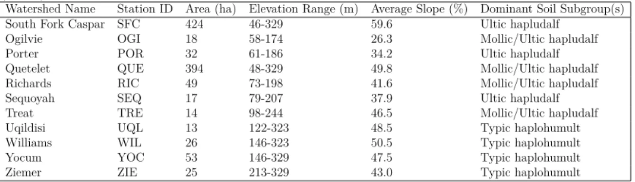
The SFC forest is comprised of third-growth coast redwood (Sequoia semper-virens), Douglas-fir (Pseudotsuga menziesii), grand fir (Abies grandis) and western hemlock (Tsuga heterophylla), there are minor components of Tanoak (Lithocarpus densiflorus), red alder (Alnus rubra) and bishop pine (pinus muricata) (Henry, 1998). Elevations range between 37 and 320 m, with average slopes ranging from 26-59% (Table 3.1). The geology at Caspar Creek consists of Franciscacn Sandstone bedrock overlain by 1 to 4 m of well-drained clay-loam ultisols and alfisols (Wagenbrenner, 2018; Henry, 1998; Carr et al., 2014). The dominant soil subgroups are Mollic haplu-dalf, Ultic haludalf and Typic hapluhumult (Dymond, 2016). Watershed characteris-tics for each of the eleven subbasins of SFC are broken down in Table 3.1. Subsurface pipeflow dynamics have been formally studied in the North Fork Caspar Creek, where it was concluded that pipe discharges are predominantly a quickflow process and pipes were said to be at depths up to 2 m within trenched swales and at the head of gullied channels in small headwater drainages (Ziemer and Alright, 1987).
Table 3.1: Physical Characteristics of SFC Sub-Watersheds. Station ID, area (ha), elevation range (m), average slope (%) and dominant soil subgroup(s) for each of the sub-watersheds in the South Fork of Caspar Creek. Excerpted from Wagenbrenner (2018).
Watershed Name Station ID Area (ha) Elevation Range (m) Average Slope (%) Dominant Soil Subgroup(s)
South Fork Caspar SFC 424 46-329 59.6 Ultic hapludalf
Ogilvie OGI 18 58-174 26.3 Mollic/Ultic hapludalf
Porter POR 32 61-186 34.2 Ultic hapludalf
Quetelet QUE 394 48-329 49.8 Mollic/Ultic hapludalf
Richards RIC 49 73-198 41.6 Mollic/Ultic hapludalf
Sequoyah SEQ 17 79-207 37.9 Ultic hapludalf
Treat TRE 14 98-244 46.5 Mollic/Ultic hapludalf
Uqildisi UQL 13 122-323 48.5 Typic haplohumult
Williams WIL 26 146-323 50.5 Typic haplohumult
Yocum YOC 53 146-329 47.5 Typic haplohumult
Ziemer ZIE 25 213-329 43.0 Typic haplohumult
av-eraged 12.0°C, with an ultimate low of 7.42°C and high of 17.5°C. The flow regime of the South Fork is typical of small forested watersheds, with flows low relative to maximum discharges most of the time and most of the flow volume, especially the sediment load, occurs during short periods of high discharge (Rice et al., 1979).
Figure 3.2: SFC Road Locations Map. Map of the South Fork Caspar Creek, including stream segments, roads and location within Jackson Demonstration State Forest.
3.2 DHSVM Background
3.2.1 DHSVM Inputs
South-west Research Station. A pixel size of 30 m was chosen because it would be large enough to encompass the stream channel and road widths found in SFC (a constraint of DHSVM) and is an efficient scale for model precision for small watersheds. A uniform vegetation representing a third growth coast redwood and fir forest was used in DHSVM. An average tree height of 45 m and leaf area index (LAI) of 7 was used based on forest stand data from JDSF (Webb, 2019).
DHSVM allows partitioning of sub-surface media or soil into different layers based on differing physical and hydraulic parameters. A sub-surface media depth of 5 m was used across SFC, based on soil core depths created for sub-surface water studies (Keepeler, 2019). In the 5 m sub-surface media a soil depth of 1.8 m was used based on maximum depth of soil in the watershed (Staff, 2019). This depth was similar to hydrologic modelling done in the North Fork of Caspar Creek, which used a 1.5 m soil depth (Carr et al., 2014). The 1.8 - 5.0 m depth was considered weathered bedrock, below 5 m we assume to be bedrock. The a priori soil parameters used in DHSVM were derived from soil hydraulic properties measured in the nearby North Fork of Caspar Creek (Carr et al., 2014) and are located in the calibration section of this report (Table 3.6).
Meteorological Forcing Files
DHSVM requires meteorological inputs at hourly or 3-hourly timesteps for air tem-perature (°C), wind speed (m/s), relative humidity (%), incoming short and long-wave radiation (W/m2) and precipitation. As advised by the model developers, DHSVM-RBM was run at a 3-hour timestep from August 2009 to September 2016.
Figure 3.3: South Fork Caspar Creek Meteorological Station. Taken Decem-ber 11, 2017.
DHSVM-RBM also allows for mul-tiple meteorological stations to be used based on location within the water-shed. One meteorological station MET1 (39°21’, 00” N, -123°44’ 20” W) and two precipitation stations SFC620 (39°20’ 29”, -123°45’ 13”) and sfc640 (39°21’ 05”, -123°43’ 41”) are located in the ex-perimental watershed (Figure 3.1). The locations of the two precipitation tions were used as meteorological sta-tions in DHSVM to most accurately rep-resent the spatial variation of rainfall throughout the watershed.
3 hours. Although PAR (photosynthetically available radiation) data is also col-lected at the meteorological station, actual incoming shortwave radiation colcol-lected by the California Irrigation Management Information System (CIMIS) Windsor Sta-tion #103, approximately 100 miles away from the research site (Figure 3.1), was used to more accurately estimate the amount of shortwave radiation reaching the site (California Department of Water Resources, 2019).
Incoming long-wave solar radiation is often computed from a general equation following the form of the Stefan-Boltzmann equation (Eq. 3.1). However, various parameterizations to estimate clear versus cloudy sky values exist (Flerchinger et al., 2009). Based on the findings of Flerchinger et al. (2009) and Wu et al. (2012), the Prata (1996) algorithm (Eq. 3.2) coupled with the Unsworth and Monteith (1975) cloud cover correction (Eq. 3.3) were chosen. Because cloud cover is not recorded at Caspar Creek, hourly estimations from the National Centers for Environmental Information (2018) Arcata Airport Station (40°58’ 41”, 124°6’ 32”) (Figure 3.1) were matched to recommended optimum values of Kclr and Kcld for the Prata-Unsworth Montheirth combination (Table 3.2).
ILR =ef fσTef f4 (3.1)
Where ef f and Tef f (K) are the effective emissivity and temperature of the atmo-sphere above the site and σ is the Stefan-Boltzmann constant.
clr = 1−(1 +w)exp(−(1.2 + 3w)
1
2) (3.2)
Where clr is the clear-sky emissivity, w= 465(Teoo),To is the near-surface air temper-ature (K) and eo is the vapor pressure (kPa) calculated as 6.11∗10
7.5Td 237.3+Td
a= (1−0.84c)clr+ 0.84c (3.3) Where cis the fraction of cloud cover and a is the effective atmospheric emissivity. Table 3.2: Cloud Cover Values. C-values for long-wave radiation calculations based on recommended values from Flerchinger et al. (2009) for a Prata-Unsworth Montheirth algorithm combination.
Arcata Cloud Cover Corresponding C-Value
Clear 0.7
Scattered 0.533
Broken 0.366
Overcast 0.2
The last meteorological input required by DHSVM-RBM is precipitation. This is measured at Caspar Creek in 0.01 inch increments. To summarize this data into a 3-hourly format, timestamps were rounded to the closest hour, summed for equivalent 3-hour timesteps and converted to meters, the required input for DHSVM.
or left blank (29.2%). These gaps were filled by either matching the two surround-ing hours, if the same (i.e. clear and clear), or linearly interpolated if different (i.e. between clear and broken).
3.3 RBM Background
The one-dimensional RBM stream-temperature model (Yearsley, 2009, 2012; Sun et al., 2015) was used to simulate historical stream temperatures in the South Fork of Caspar Creek. RBM solves time dependent equations for the conservation of thermal energy between the air-water interface using a semi-Lagranagian method (Yearsley, 2009, 2012). Water inflow and outflow for each stream segment, as well as energy budget components, are produced as outputs from DHSVM for RBM. These outputs, and parameters dictating initial upstream temperatures (Mohseni Parameters) and stream speed and depth (Leopold Parameters), are used to complete the calculations. Downstream water temperatures are estimated using solar radiation, net longwave radiation, sensible heat flux, latent heat flux, groundwater and advected heat from adjacent tributary segments. The water parcels are tracked through the river basin to determine results for points throughout the stream network.
The newest version of RBM allows vegetation height, buffer width, a monthly ex-tinction coefficient, percent overhanging vegetation, canopy bank distance and chan-nel width to be manipulated for each stream segment. Part A in Figure 3.4 shows a 3-D view of the riparian shading setup RBM uses to calculate the shadow length of the buffer canopy at each time step using solar altitude (φ), azimuth (θsun), stream
azimuth (θstreams), bank height (Hbank) and vegetation height (Htree). Part B depicts
Figure 3.4: RBM Riparian Shading. Diagram of how riparian shading over stream surfaces occurs in RBM. Excerpted from (Sun et al., 2015).
3.3.1 RBM Inputs
Mohseni Parameters
RBM requires estimates of initial headwater temperatures. Yearsley (2012) tested two methods to provide these estimates, daily soil temperature and the Mohseni et al. (1998) nonlinear regression model relating air and stream temperature, and found no improvements to model results using soil temperature. For this reason we used the Mohseni et al. (1998) method. The Mohseni nonlinear regression analysis model is as follows
Ts =µ+
α−µ
1 +eγ(β−Tsmooth) (3.4)
Where Ts is the simulated stream temperature,µ is the estimated minimum stream temperature, Tsmooth is the smoothed air temperature, α is the maximum actual stream temperature,γ is a measure of the steepest slope of the function, β is the air
temperature at the inflection point andγ is a function of the slope tanθ at said point
of inflection.
γ = 4 tanθ
α−µ (3.5)
Tsmooth =λ∗Tair(t) + (1−λ)∗Tair(t−1) (3.6) ForTsmooth, the value ofλis determined by the highest possible correlation coefficient
between smoothed air temperature and measured water temperature.
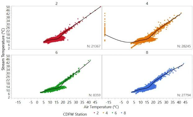
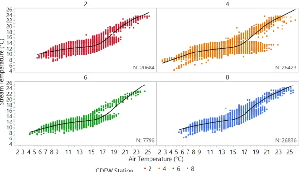
evaluation using JMP Pro 13 of all air and water temperature values can be seen in (Figure 3.5).
Figure 3.5: Development of Mohseni Parameters - Outliers Included. Air temperature (°C) vs. stream temperature (°C), with outliers included, to calculate Mohseni headwater parameters.
Figure 3.6: Development of Mohseni Parameters - Outliers Excluded. Air temperature (°C) vs. stream temperature (°C), with outliers excluded, used to estab-lish Mohseni headwater parameters.
These values were then used in equations 3.4, 3.5 and 3.6 to estimate parameters used by RBM for initial headwater stream temperatures. These parameters are pre-sented in Table 3.3, as well as the final parameter set used in RBM. Final parameters were determined by incrementally adjusting the Mohseni and Leopold variables to find those that resulted in stream temperature estimates closest to measured readings at the outlet of the mainstem (QUE).
Table 3.3: Mohseni Parameters. Mohseni variables produced using CDFW data.
CDFW Station α(°C) θ (°C) γ β (°C) µ (°C) λ
2A 23.63 22.75 0.234 18.5 7.43 0.99
4B 23.63 22.50 0.1145 18.00 4.15 0.90
6C 22.86 22.50 0.145 19.00 7.43 1.10
8D 24.01 22.75 0.213 17.5 6.22 1.20
Leopold Parameters
RBM uses coefficients relating velocity and depth to river discharge to establish hydraulic characteristics based on the works of Leopold and Maddock (1953). These coefficients can be set for each stream segment or generalized to the entire watershed. Equations 3.7 and 3.8 are the power equations used to relate depth and velocity to discharge. Where D is depth, v is velocity, Q is discharge and a, b, c and d are empirical constants determined from discharge rating curves. RBM also allows minimum stream speeds to be set, to account for the potential for abnormally low stream speeds because these equations are constant in time.
D=aQb (3.7)
v =cQd (3.8)
The data needed to establish these relationships has not been established at SFC. Empirical equations to predict stream width and depth exist (Allen et al., 1994; Ames et al., 2009); however, these equations were determined to be too uncertain due to the different hydrologic conditions where they were developed (i.e. snow). Therefore, historical stage and discharge readings, as well as known weir dimensions, were used to back out estimates of these parameters.
Figure 3.7: Leopold Parameters - Cross Section. Cross section just upstream of the SFC weir, using a 2-meter resolution DEM, to estimate natural channel width and depth estimations.
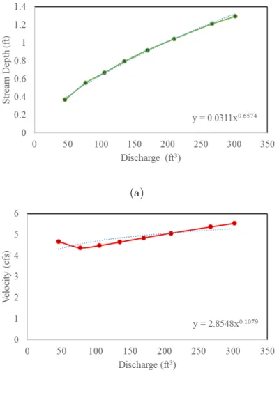
(a)
(b)
Figure 3.8: Leopold Parameters - Relationships. (a) Depth to stream discharge and (b) velocity to stream discharge relationship calculated for the South Fork of Caspar Creek.
Table 3.4: Leopold Parameters. Final Leopold parameters used for calibration and temperature simulations.
Coefficient Exponent Minimum
Velocity (ft3/sec) 2.85 0.11 0.25
Depth (ft) 0.03 0.66 0.50
Expected ranges for the exponent termsb andd reported by Chapra (1997) range
above and below these ranges, highlighting a potential source of error. No expected ranges are reported for the coefficient terms.
Riparian Shading
As mentioned, RBM allows various riparian characteristics to be altered for each stream segment, including: tree height (m), buffer width (m), monthly extinction coefficient (similar to LAI), overhang coefficient (the percentage of tree height that overhangs the stream), canopy bank distance (m) and channel width (m). Riparian characteristics used in the initial pre-harvest simulation are in Table 3.5. Buffer widths were chosen based on California FPRs. However, RBM does not allow for the creation of core, inner and outer zones as prescribed by the California FPRs, therefore presenting a limitation to the study. Tree height was estimated by Caspar personnel from Lidar data within the 150 foot Class I WLPZ. An average monthly extinction coefficient forPseudotsuga menziesii was taken from the work of Thomas and Winner (2011) and the overhang coefficient was based on the mean percent canopy density for SFC (California Department of Fish and Wildlife, 2006). The monthly extinction coefficient can be adjusted month to month, however these values were kept constant, like in the works of Truitt (2018), to represent a coniferous dominated forest.
Table 3.5: Initial Riparian Characteristics. Riparian characteristics used for initial, third-growth conditions
Class I Class II Class III
Buffer Width (ft) 100 85 25
Channel Width (m) 4 2 1
Tree Height (m) 50.6 50.6 50.6
Monthly Extinction Coefficient 0.525 0.525 0.525
Overhang Coefficient 0.90 0.90 0.90
3.4 Model Calibration
3.4.1 RBM
For most coastal western US areas, stream temperatures are generally highest during summer, coinciding with when flows are lowest and energy inputs are highest (clear skys). Therefore, similar to the works of Sun et al. (2015), the period of May 1st to September 30th was evaluated to capture this critical time period for aquatic species. In order to gauge model fit, the Nash-Sutcliffe Efficiency (NSE) (Eq. 3.9) was used to assess the goodness of fit and the root mean square error (RMSE) (Eq. 3.10) was used to assess the quality of the fit. When NSE values are equal to 1.0, simulated values perfectly match measured values. When NSE values are ≤ 0 the
simulated values are worse than the measured mean. Lower RMSE values indicate a better fit.
N SE = 1−
n P t=1(
Tst −Tat)
2
n P t=1( ¯
Ta−Tat)2
(3.9)
RM SE =
v u u u t n P t=1(
Tst−Tat)2
n−4 (3.10)
Where,Tstis the simulated stream temperature at time t,Tat is the actual stream
7-day average temperatures (MWAT) and maximum of the 7-day maximum temper-atures (MWMT) were calculated to compare to measured values. Cao et al. (2016) addresses that although the use of a 3-hour timestep has the potential to limit RBMs ability to capture daily maxima, it does not do so significantly enough to recommend against using RBM output to calculate the MWMT. Additionally, the MWAT and MWMT are used by the EPA and many other government agencies to identify viable water temperatures for aquatic species, making their use in these results more widely applicable to decision makers.
3.4.2 DHSVM
Calibration of DHSVM was based on fit to measured streamflow at the outlet of SFC and RIC watersheds (Figure 3.2). A 3 hour time step was used for DHSVM simulations. DHSVM was run from 2010 to 2016 HY with the 2010 HY used as a spin-up period to equilibrate the initial water balance. DHSVM was calibrated for the 2011 to 2013 HY and verified for the 2014 to 2016 HY. HY at Caspar Creek runs from August 1 to July 31.
The model was calibrated by adjusting four sensitive soil hydraulic parameters: (1) lateral hydraulic conductivity, (2) exponent of decay (an exponent of the nat-ural logarithm describing the decrease in hydraulic conductivity by depth of soil), (3) porosity of the soil matrix, and (4) vertical hydraulic conductivity. These four parameters, and the range of values for each parameter selected, were based on prelim-inary model trials that demonstrated competence at achieving model fit to measured streamflow.
hydrologic models that uses squared values making them sensitive to high streamflow events. The EREL value modifies the NSE as relative deviations, adjusting model fit based on size of event, thus better reflecting fit of the entire series and reducing the influence of the absolute differences during high flows (Surfleet et al., 2012). As a result, EREL values are more sensitive to systematic over- or under-prediction, in particular during low flow conditions (Krause et al., 2005), with higher values indicating higher model fit. Calibration was based on achieving high values of EREL metrics (>0.9), while maintaining reasonable NSE values (>0.6). The primary stream
temperature analysis in this study was summer stream temperatures during lowflow periods. The EREL is a better metric for smaller streamflows then NSE.
Erel = 1− n P i=1(
Oi−Pi
Oi )
2
n P t=1(
Oi−O¯
¯ O )
2 (3.11)
WithO observed andP predicted values.
Table 3.6: DHSVM Variables. A priori and calibrated parameters for SFC 2011-2016 HY. A priori parameters are in parenthesis. HC= hydraulic conductivity.
Depth(m) Porosity Vertical HC
(m/s) Exponent of Decay HorizontalHC (m/s) 0 - 1.8 (0.5) 0.46 (2.2x10⁻⁵)
1.9x10⁻⁴
3.9 (2.2x10⁻⁵) 9.0x10⁻³ 1.8 - 5.0 (0.1) 0.09 (2.2x10⁻⁵)
1.9x10⁻⁴
3.9 (2.2x10⁻⁶) 1.0x10⁻⁶
3.5 Modeling Scenarios
report were guided based on input from an advisory committee including California Department of Forestry and Fire Protection and US Forest Service Caspar Creek staff. The simulations run are broken into three sections- canopy reductions, the harvest scenario and an experimental riparian reach design.
3.5.1 Canopy Reduction
The first set of scenarios decreased tree height, the monthly extinction coefficient (similar to LAI) and canopy overhang to 80, 65, 50, 25 and 0% of the initial conditions along all stream classes. Two extreme scenarios, clear cutting the entire watershed (including the buffer areas) and treating the watershed as if it had been preserved for old growth were also simulated. Table 3.7 outlines the riparian characteristics used for each canopy scenario. For all scenarios the buffer width and channel width remained at the initial conditions based on stream class (Table 3.5).