Sharif University of Technology
Scientia IranicaTransactions E: Industrial Engineering www.scientiairanica.com
A four-phase algorithm to improve reliability in
series-parallel systems with redundancy allocation
A. Ghafarian Salehi Nezhad
a;, A. Eshraghniaye Jahromi
a, M.H. Salmani
aand F. Ghasemi
ba. Department of Industrial Engineering, Sharif University of Technology, Tehran, P.O. Box 14588-89694, Iran.
b. Department of Industrial Engineering and Management Systems, Amirkabir University of Technology, Tehran, P.O. Box 15875-4413, Iran.
Received 26 November 2012; received in revised form 12 August 2013; accepted 20 August 2013 KEYWORDS
Reliability optimization; Redundancy allocation;
Series-parallel system; Ant colony
optimization; Heuristic algorithms; Parameter design; Taguchi approach.
Abstract. In general, reliability is the ability of a system to perform and maintain its functions in routine, as well as hostile or unexpected, circumstances. The Redundancy Allocation Problem (RAP) is a combinatorial problem which maximizes system reliability by discrete simultaneous selection from available components. The main purpose of this study is to develop an eective approach to solve RAP, expeditiously.
In this study, the basic assumption is considering Erlang distribution density for component failure rates. Another assumption is that each subsystem can have one of cold-standby or active redundancy strategies. The RAP is a NP-Hard problem which cannot be solved in reasonable time using exact optimization techniques. Therefore, an approach that combines an Ant Colony Optimization (ACO) algorithm as a meta-heuristic phase, and three other heuristics, is used to develop a solving methodology for RAP. Finally, to prove the eciency of the proposed approach, some well-known benchmarks in the literature are solved and discussed in detail.
c
2014 Sharif University of Technology. All rights reserved.
1. Introduction
Reliability problems are well-known problems in theory and practice in which the main objective is improving system reliability to obtain the most eective system possible. In this area, the Redundancy Allocation Problem (RAP) is a favorite problem, which has at-tracted the attention of engineers and other researchers in planning the selection of components for a system, simultaneously, and where they endeavor to combine various components by dierent strategies. Generally, this problem is formulated in order to maximize system reliability in which some predetermined constraints,
*. Corresponding author. Tel: +98 936 337 7547; Fax: +98 331 262 4268
E-mail address: a [email protected] (A. Ghafarian Salehi Nezhad)
such as total weight, total cost, and total volume, are satised. Due to various practical applications for RAP, its attractiveness has further grown over the last decades, in theory. In general, it is possible to categorize series-parallel systems into three major parts: reliability allocation, redundancy allocation, and reliability and redundancy allocation. In the reliability allocation problems, the reliability of the components is determined, such that the consump-tion of a resource under a reliability constraint is minimized, while the redundancy allocation problem generally involves the selection of components and redundancy levels to maximize system reliability, given various system-level constraints [1]. In fact, we can implement two approaches to improve the reliability of such a system using RAP. The rst is to increase the reliability of system components, while the second is using redundant components in various subsystems in
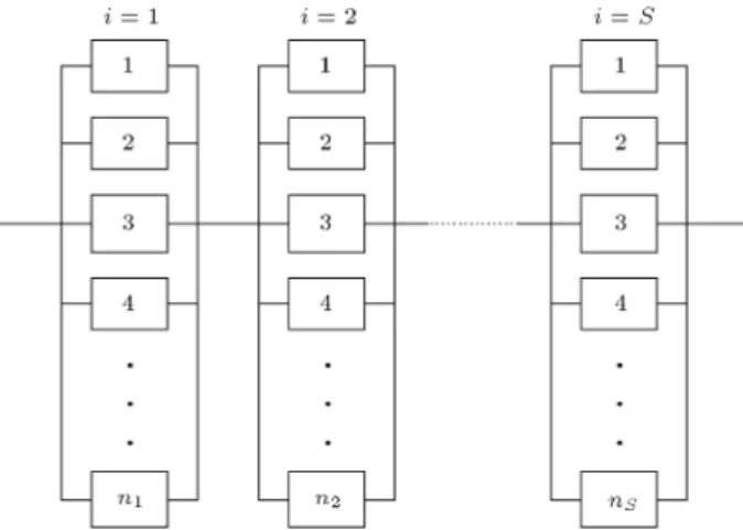
Figure 1. Structure of series-parallel systems.
the system [2,3]. Mainly, This problem has four major inputs: = [izi] which represents the failure rate for
component zi in subsystem i, C = [Cizi] and W =
[Wizi] which are the cost and weight of component zi
for subsystem i, respectively, and = [i(t)] which is
switch reliability in subsystem i at a predetermined time, t. The general structure of the series-parallel system is shown in Figure 1, where i indicates the index of each subsystem.
The general structure of this paper is as follows. First, a concise and comprehensive literature review is presented for various studies undertaken over the last decades. Afterwards, an appropriate mathematical model is developed in Section 3. Following these sections, we present developed heuristics algorithms, which are claried in detail in Section 4. Then, the proposed model is tested by a benchmark problem in the computational results part in Section 5. Finally, this paper is recapitulated in Section 6.
2. Literature review
Reliability is a favorite, appropriate tool in all in-dustries where its importance cannot be concealed. Various applications of reliability problems in practical areas have resulted in the attractiveness of such kinds of problems in theoretical areas over the last decades, and various models and algorithms are presented in the literature which can generate appropriate solutions for reliability problems, expeditiously. As a matter of fact, it can be said that RAP is one of the most important problems to cover various shortages in industry. It is proven that RAP in series systems is a NP-complete problem [4]. One of the most important studies was presented by Coit and Smith [5] who reviewed dierent optimization approaches. Their paper proposed a new approach, based on the Genetic Algorithm (GA), which can solve general classes of the redundancy allocation problem. Along with these studies, various researchers endeavored to develop a
model to allocate redundant components to subsystems to increase system reliability [6,7]. Another noticeable study was developed to maximize system reliability in a series system with multiple-choice constraints incorporated into each subsystem [8]. Sung and Cho also considered an applicable constraint, which was the system budget in their mathematical model. This problem was formulated as a nonlinear binary integer programming problem, which is NP-hard. In 2009, a Multi-state Series-Parallel System (MSPS) with capacitated binary components, which could provide dierent multi-state system performance levels, was presented by Ramirez-Marquez and Coit [9]. In to-day's market, it is very important to optimize costs, and Bris, et al. presented research which focused on this subject [10]. Yalaoui, et al. developed a model for series-parallel reliability problems, which tried to minimize a concave objective function [11]. Ruan and Sun [12] proposed an exact method to minimize total costs in series reliability systems with multiple component choices. This model was based on the nonlinear integer programming problem approach with a non-separable constraint function. Nahas and Nourelfath [13] developed an ant system to solve the reliability optimization problem for a series system with multiple-choice constraints incorporated at each subsystem, to maximize system reliability subject to the system budget. Zhao, et al. [14] developed a multi-objective Ant Colony System (ACS) meta-heuristic to provide solutions for the reliability optimization problem of series-parallel systems. In this type of problem, selection of components with multiple choices and redundancy levels to produce maximum benets was assumed, where the cost and weight constraints at the system level were considered. Another study con-centrated on modeling the reliability and redundancy maintenance of queening systems using controlled semi-Markov processes [15]. In that paper, they attempted to nd the conditional extreme of the considered functional and determine the structure of the distribu-tions, which prove a corresponding extreme. A study by Ahmadizar and Soltanpanah [16] concentrated on choosing one technology for each subsystem in order to maximize the reliability of the whole system, subject to the available budget. Furthermore, they proposed an ecient ACO approach to generate a solution using an ant based algorithm on both pheromone trails modied by previous ants, and heuristic information considered as a fuzzy set.
In this study, two main goals are considered. The rst is presenting a mathematical model which is simpler in comparison to the ones in the literature. In other words, it would be easier to solve this model using common techniques to solve optimization problems. The second is developing an eective algorithm for resulting appropriate solutions in a reasonable time
period. This algorithm is comprised of four stages, as follows:
1. Use of an ACO algorithm which tries to nd an initial solution;
2. By replacing the used component in each subsystem with another to nd a better-o solution from the view point of the objective function;
3. Modifying the determined strategy among subsys-tems to generate a better-o solution from the view point of the objective function;
4. Using a tabu search algorithm to nd a more appropriate solution among the adjacencies of a generated solution.
3. Mathematical model for RAP
As various models in the literature, we consider two dierent strategies for components of subsystems in RAP: active and standby. In the rst, which is active strategy, all redundant components will start to work simultaneously from time zero. On the other hand, according to the various categories of redundancy strategies, there are three dierent types of cold, warm and hot strategies, instead of the second strategy which is known as the standby strategy. In the cold one, components do not fail before their start time of operation. In warm variants, in comparison to cold ones, it will be more likely that components will fail before starting to operate the system. If we use the hot variant, whether the components work or not, their failure rates will be constant anyway. Therefore, we can propose a mathematical model to consider two dierent types of active and standby strategies in our problem. However, in the standby redundancy arrangement, the redundant components are sequentially used in the system at component failure times, and each redundant component in the standby systems can be operated only when it is switched on. When the component in operation fails, one of the redundant units is switched on to continue the system operation [17].
By considering two dierent proposed strategies, the following denition for three important parameter sets in our mathematical model can be presented: A Consists of all subsystems that are
working, based on an active redundant strategy.
S Includes subsystems that have a standby-cold redundant strategy. N Represents those subsystems that do
not have any redundant strategy. In other words, each subsystem in this group has just one component.
Other notications, parameters, and variables are as
follows:
S Number of subsystems;
i Index of subsystems where i = 1; 2; ; si;
ni Number of components used in
subsystem i;
N Set of all ni(n1; n2; ; nS);
nmax;i Upper bound of ni(ni nmax;i8i);
mi Number of available component choices
for a subsystem, i;
zi Index of used component (among
dierent mi types of components) in
subsystem i(zi 2 f1; 2; ; mig);
Z Set of all zi(z1; z2; ; zS);
t Mission time;
R(t; z; n) System reliability at time t for designing vectors, z and n; ri;zi(t) Reliability of component zi for
subsystem i at time t;
i;zi; Ki;zi Scale and shape parameters for the
Gamma distribution of component zi
in subsystem i, respectively;
C; W System level constraint limits for cost and weight, respectively;
Ci;zi; Wi;zi Cost and weight for component zi in
subsystem i, respectively;
i(t) Failure/detection switching reliability
of subsystem i at time t.
According to these denitions, Relations (1), (2), and (3) are proposed in this study.
max R(t; z; n):
S.T. : (1)
S
X
i=1
Ci;zini C; ni2 f1; 2; ; nmax; ig; (2)
S
X
i=1
Wi;zini W; ni2 f1; 2; ; nmax; ig; (3)
where, Eqs. (2) and (3) will enforce the model not to exceed total cost and weight from predetermined upper bounds, respectively. Moreover, according to our active and standby-cold redundant strategies, R(t; z; n) will be calculated by Eq. (4):
R(t; z; n) =Y
i2A
Y
i2S
0
@ri;zi(t)+
0 @nXi 1
x=1 t
Z
0
x
ifi;z(x)i(u)ri;zi(t u)du
1 A
1 A
Y
i2N
ri;zi(t): (4)
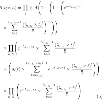
According to [17], we can calculate R(t; z; n) by the following equation:
R(t; z; n) =Y
i
2 A 1 1 e i;zit
KiX;zi 1
l=0
(i;zi t)l
l!
!ni!!
Y
i2S
e i;zit
Ki;ziX1
l=0
(i;zi t)l
l! + i(t)
(ki;ziXni) 1
l=ki;zi
e i;zit(i;zi t)l
l!
!!
Y
i2N
0
@e i;zit
Ki;ziX1
l=0
(i;zi t)l
l! 1 A :
(5) As mentioned before, RAP is a NP-complete problem. Therefore, we need to develop eective algorithms to solve this model, expeditiously. In the following section, we will propose a four phase algorithm to solve our model, consisting of Relations (1), (2), and (3). It is necessary to mention that Relation (1) will be replaced by Relation (5).
4. Heuristic algorithm to solve RAP
To encode the solution, we must consider a matrix in such a way that the strategy of each subsystem, type of used component, and number of used components are determined. Therefore, we utilize a matrix with three rows and S columns. In Figure 2, an example of encoding the solution is shown with ten subsystems.
For instance, in Figure 2, the third subsystem is working based on the active redundancy strategy, where ve components of the fourth type of component are selected for this subsystem.
Figure 2. Encoding Solution for a Sample Problem.
4.1. First phase: Ant colony optimization algorithm
Generating an appropriate solution in a reasonable time period is an important goal which has resulted in raising the attractiveness of ant colony algorithms. This type of algorithm was rstly introduced by Dorigo, et al. [18]. The main idea of ant systems is based on the behavior of natural ants that succeed in nding the shortest path from their nest to food sources by communicating via a collective memory consisting of pheromone trails. Ants tend to follow a path with a high pheromone level, when many ants move in a common area, and they move randomly when no pheromone is available. On the other hand, ants do not choose their directions based on the level of pheromones exclusively, but rather take the proximity of the nest and food source into account, respectively. This process is illustrated in Figure 3.
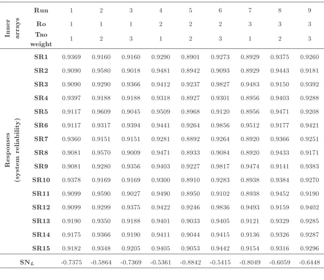
To tune the algorithm parameters, we used the well-known Taguchi approach, \Ro" and \Tao Weight", as the parameters which can be controlled, completely. Moreover, \Lambda Weight" will be cal-culated by subtracting Tao Weight from one. Table 1 shows the parameter levels using the Taguchi approach. Orthogonal array for controllable factors with system reliability and Signal to Noise ratio (SN) values are shown in Table 2. Noticeably, we use SNL because we want to increase system reliability.
SNL = 10 log 1n n
X
i=1
(System Reliability)2 i
! :
(6)
Figure 3. (a) Real ants follow a path between nest and food source. (b) An obstacle appears on the path; ants choose whether to turn left or right with equal probability. (c) Pheromone is deposited more quickly on the shorter path. (d) All ants have chosen the shorter path.
Table 1. Factors and levels for the parameter design. Controllable
factors Levels
Ro Low (0.01) Medium (0.05) High (1) Tao weight Low (0.2) Medium (0.5) High (0.8) Lambda weight = 1 Tao weight
Table 2. Parameter design with inner arrays.
Inner arra
ys
Run 1 2 3 4 5 6 7 8 9
Ro 1 1 1 2 2 2 3 3 3
Tao
weight 1 2 3 1 2 3 1 2 3
Resp
onses
(system
reliabilit
y)
SR1 0.9369 0.9160 0.9160 0.9290 0.8901 0.9273 0.8929 0.9375 0.9260 SR2 0.9090 0.9580 0.9018 0.9481 0.8942 0.9093 0.8929 0.9443 0.9181 SR3 0.9090 0.9290 0.9366 0.9412 0.9237 0.9827 0.9483 0.9150 0.9392 SR4 0.9397 0.9188 0.9188 0.9318 0.8927 0.9301 0.8956 0.9403 0.9288 SR5 0.9117 0.9609 0.9045 0.9509 0.8968 0.9120 0.8956 0.9471 0.9208 SR6 0.9117 0.9317 0.9394 0.9441 0.9264 0.9856 0.9512 0.9177 0.9421 SR7 0.9360 0.9151 0.9151 0.9281 0.8892 0.9264 0.8920 0.9366 0.9251 SR8 0.9081 0.9570 0.9009 0.9471 0.8933 0.9084 0.8920 0.9433 0.9171 SR9 0.9081 0.9280 0.9356 0.9403 0.9227 0.9817 0.9474 0.9141 0.9383 SR10 0.9378 0.9169 0.9169 0.9300 0.8910 0.9283 0.8938 0.9384 0.9270 SR11 0.9099 0.9590 0.9027 0.9490 0.8950 0.9102 0.8938 0.9452 0.9190 SR12 0.9099 0.9299 0.9375 0.9422 0.9246 0.9836 0.9493 0.9159 0.9402 SR13 0.9190 0.9350 0.9188 0.9401 0.9033 0.9405 0.9121 0.9329 0.9285 SR14 0.9175 0.9366 0.9190 0.9411 0.9044 0.9415 0.9136 0.9326 0.9287 SR15 0.9182 0.9348 0.9205 0.9405 0.9053 0.9442 0.9154 0.9316 0.9296 SNL -0.7375 -0.5864 -0.7369 -0.5361 -0.8842 -0.5415 -0.8049 -0.6059 -0.6448
Figure 4. Main eects plot for SN ratios.
We know that the best parameters result in higher SNL,
and this notication leads us to determine values as Ro = 0:05, Tao Weight = 0:8, and Lambda Weight = 0:2. These results are shown in Figure 4.
4.1.1. The procedure of the ant colony algorithm
Step 1 (Initialization). All parameters in an ant colony algorithm are primarily initialized. The algo-rithm is terminated when it reaches 2000 iterations.
The number of ants will be determined by the num-ber of subsystems. Pheromone information weight is 0.80 and component failure rates information weight is 0.2. Pheromone values () on each path are initialized with random values drawn from interval [0:10; 0:25]. It is noticeable that pheromone values are considered a matrix, where its dimensions are the maximum number of component types among subsystems plus one, and the number of subsys-tems. Therefore, with this matrix, it is possible to determine subsystem strategies, component types, and number of components according to the value of the pheromones. Moreover, the value of , which is the rate of pheromone updating, is equal to 0.05, and random number, q, will be generated in interval [0; 1].
Step 2 (Initial solution construction). A random initial solution (S0) is generated. It is noticeable
that the redundant strategy of each subsystem is determined by a generated random number which is less than or greater than the related pheromone value. Moreover, the component type will be
determined according to Eq. (7): i = arg max
j 0:8
ij
P
jij 0:2
ij
P
jij
!! ; 8i = 1; 2; ; S; (7) where, the arg function determines the index that has the maximum value of parenthesis. In this equation, S is the number of used subsystems, and i;j and i;j are pheromone rate and problem
information rate of path (i; j), respectively. On the other hand, the number of components will be determined according to Constraints (2) and (3), while it is trying to maximize all the pheromones. Moreover in this step, the value of the objective will be calculated according to Eq. (5).
Step 3 (Local improvement). In this step, a swapping procedure is used. First, according to a generated random number, one of the used compo-nents of each subsystem will be determined and will be replaced by another component, and it is not important whether it is used in a related subsystem or not. This swapping procedure will be repeated while no possible replacement can be occurred.
Step 4 (Best solution improvement). After all ants complete their solutions, the best solution in iteration is selected, and the algorithm tries to improve, such as in Step 3.
Step 5 (Pheromone updating). The best solution is used to update the pheromone matrix, where Eqs. (8) and (9) are utilized to update this matrix: ij(t + 1) = (1 ) ij(t) + (10 )ij(t); (8)
ij(t) =
(
1 if (i; j) 2 the best solution
0 Otherwise (9)
To prevent the algorithm from converging to a solution, when the value of the pheromone becomes less than 0.001, it will change to a new value that is selected randomly from [0:10; 0:20]. This interval was the best among more than 10,000 iteration and 20 dierent problems.
4.2. Second phase
In this phase, the best generated solution in the previous phase will be considered as an initial solution. Afterwards, for each subsystem, i, all mi components
will be assigned, one by one. For all new systems, the value of the objective function will be generated. Then, for the one generated system whose value of objective function is better than the initial solution, the initial solution will be replaced with the related solution. The best solution in this phase will be considered an initial
solution for the next phase. It is noticeable that for each step of this phase, the solution should be feasible according to the proposed constraints.
4.3. Third phase
This phase has the same approach as the previous one, where the only dierence is to assign dierent strategies for each subsystem to generate a new feasible solution. In this phase, all comparisons between the initial solution and new feasible solutions will be done to select the best one.
4.4. Fourth phase
As the other phase, this phase will improve the best founded solution before this step by searching among the adjacencies of each solution. Suppose that the solution at the end of phase three is named the best solution. In the structure of this solution, the subsystems with maximum and minimum values of reliability are called Max and Min, respectively, where the number of components in each of these two subsys-tems is supposed to be nmaxand nmin, correspondingly.
Therefore, we can dene the structure of the best solution as the following relation:
Best solution = fnmax; nmin; n g: (10)
Now, we can dene following adjacencies:
fnmax+ 1; nmin+ 1; n g; (11)
fnmax+ 1; nmin; n g; (12)
fnmax; nmin+ 1; n g; (13)
fnmax 1; nmin+ 1; n g; (14)
fnmax 1; nmin+ 2; n g; (15)
fnmax 2; nmin+ 1; n g; (16)
fnmax 2; nmin+ 2; n g; (17)
fnmax 2; nmin+ 3; n g: (18)
Now, for any feasible solution among these adjacencies, if any better-o solution, in comparison to the best solution, until this step, is found, it will be replaced and considered as the best solution till now.
This phase will be repeated while no better feasible solution can be found for RAP. Then, phases 2 to 4 will be repeated again for iteration.
5. Computational results
To evaluate and validate the proposed algorithm for RAP, a general benchmark example is solved. This
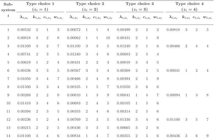
Table 3. Problem parameters.
Sub-system i
Type choice 1 (zi= 1)
Type choice 2 (zi= 2)
Type choice 3 (zi= 3)
Type choice 4 (zi= 4)
i;zi ki;zi ci;zi wi;zi i;zi ki;zi ci;zi wi;zi i;zi ki;zi ci;zi wi;zi i;zi ki;zi ci;zi wi;zi
1 0.00532 2 1 3 0.00072 1 1 4 0.00499 2 2 2 0.00818 3 2 5
2 0.00818 3 2 8 0.00062 1 1 10 0.00431 2 1 9
3 0.01330 3 2 7 0.01100 3 3 5 0.01240 3 1 6 0.00466 2 4 4
4 0.00741 2 3 5 0.01240 3 4 6 0.00683 2 5 4
5 0.00619 1 2 4 0.00431 2 2 3 0.00818 3 3 5
6 0.00436 3 3 5 0.00567 3 3 4 0.00268 2 2 5 0.00041 1 2 4
7 0.01050 3 4 7 0.00466 2 4 8 0.00394 2 5 9
8 0.01500 3 3 4 0.00105 1 5 7 0.01050 3 6 6
9 0.00268 2 2 8 0.00010 1 3 9 0.00041 1 4 7 0.00094 1 3 8
10 0.01410 3 4 6 0.00683 2 4 5 0.00105 1 5 6
11 0.00394 2 3 5 0.00355 2 4 6 0.00314 2 5 6
12 0.00236 1 2 4 0.00769 2 3 5 0.01330 3 4 6 0.01100 3 5 7
13 0.00215 2 2 5 0.00436 3 3 5 0.00665 3 2 6
14 0.01100 3 4 6 0.00834 1 4 7 0.00355 2 5 6 0.00436 3 6 9
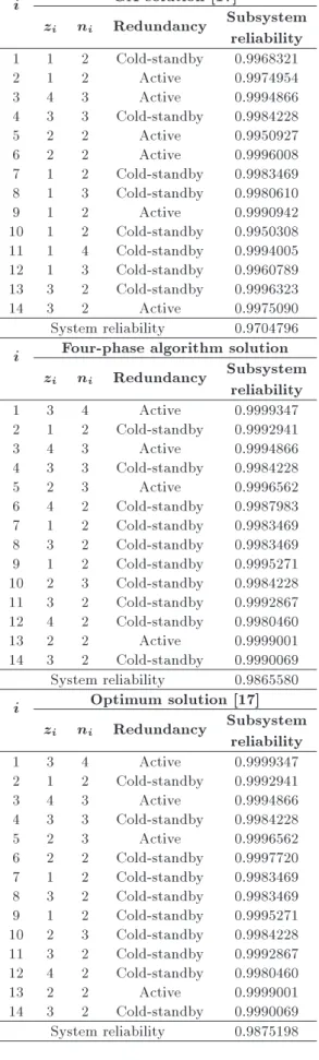
example is compromised of 14 parallel subsystems with 3 or 4 components for each subsystem. For this example, costs, weights, and Gamma distribution parameters are shown in Table 3. In this problem, the main objective is maximizing total system re-liability at time 100 hours, with the constraint of maximum allowed values, 130 and 170, for total cost and total weight, respectively. Also, both active and standby strategies are possible for each subsystem, where the reliability of each switch is supposed to be 0.99 [17].
This problem is solved by the proposed algorithm and the results are shown in Table 4. These results indicate the eciency of this algorithm to solve RAP. As is obvious in this table, the proposed algorithm generates better-o solutions in comparison to other algorithms in the literature. Moreover, if we compare the optimum solution with the generated solution of this study, we can understand that for all subsystems, the same strategy and number of components are gained.
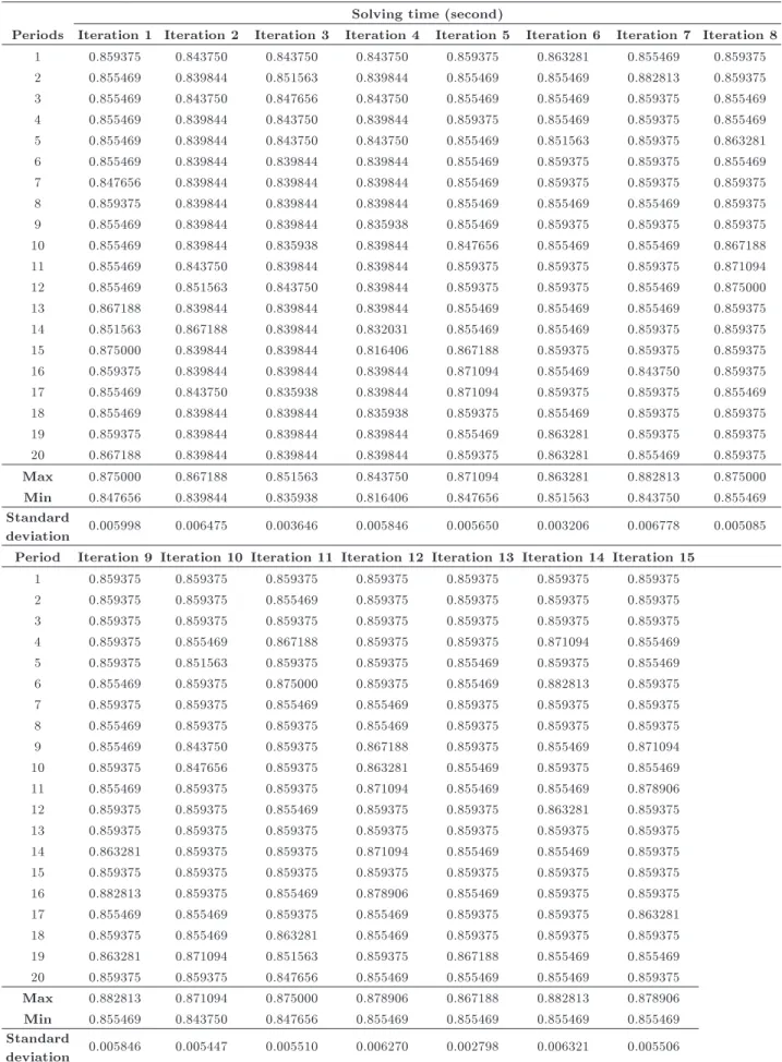
To prove the eectiveness of the presented algo-rithm, 300 iterations, consisting of 20 periods and 15 iterations per period, are applied to the benchmark (Table 5).
These results indicate that applying the proposed algorithm for diverse iterations results in an
appro-priate average for solving time with low standard deviation. To prove this notication, two statistical tests are presented.
Average solving time for 300 iterations is 0.855, and its standard deviation is 0.0092. Now, while time is expected to have normal distribution, we do the following two statistical tests:
(
H0: = 0:85
H1: > 0:85 (19)
We know that t = x 0
s=pn is a t-student statistic that can
be used to analyze this statistical test. If this value was greater than t(n 1;1
2), hypothesis H0will be rejected
with a probability of (1 =2). According to the values and dierent iterations, we have:
t = X 0 s=pn =
0:855 :85
:0092 = 0:54: (20) Now, if we consider doing this test with = 0:05, t(299;0:975) = 1:97 would be determined, and,
there-fore, we cannot reject H0 with a probability of
0.975.
Noticeably, we can do the following statistical test for standard deviation, and we should use the chi-squared statistics, X2 = Pni=1(xi x)2
2
Table 4. Comparing the generated solution with another one in the literature.
i GA solution [17]
zi ni Redundancy Subsystem
reliability 1 1 2 Cold-standby 0.9968321
2 1 2 Active 0.9974954
3 4 3 Active 0.9994866
4 3 3 Cold-standby 0.9984228
5 2 2 Active 0.9950927
6 2 2 Active 0.9996008
7 1 2 Cold-standby 0.9983469 8 1 3 Cold-standby 0.9980610
9 1 2 Active 0.9990942
10 1 2 Cold-standby 0.9950308 11 1 4 Cold-standby 0.9994005 12 1 3 Cold-standby 0.9960789 13 3 2 Cold-standby 0.9996323
14 3 2 Active 0.9975090
System reliability 0.9704796 i Four-phase algorithm solution
zi ni Redundancy Subsystem
reliability
1 3 4 Active 0.9999347
2 1 2 Cold-standby 0.9992941
3 4 3 Active 0.9994866
4 3 3 Cold-standby 0.9984228
5 2 3 Active 0.9996562
6 4 2 Cold-standby 0.9987983 7 1 2 Cold-standby 0.9983469 8 3 2 Cold-standby 0.9983469 9 1 2 Cold-standby 0.9995271 10 2 3 Cold-standby 0.9984228 11 3 2 Cold-standby 0.9992867 12 4 2 Cold-standby 0.9980460
13 2 2 Active 0.9999001
14 3 2 Cold-standby 0.9990069 System reliability 0.9865580 i Optimum solution [17]
zi ni Redundancy Subsystem
reliability
1 3 4 Active 0.9999347
2 1 2 Cold-standby 0.9992941
3 4 3 Active 0.9994866
4 3 3 Cold-standby 0.9984228
5 2 3 Active 0.9996562
6 2 2 Cold-standby 0.9997720 7 1 2 Cold-standby 0.9983469 8 3 2 Cold-standby 0.9983469 9 1 2 Cold-standby 0.9995271 10 2 3 Cold-standby 0.9984228 11 3 2 Cold-standby 0.9992867 12 4 2 Cold-standby 0.9980460
13 2 2 Active 0.9999001
14 3 2 Cold-standby 0.9990069 System reliability 0.9875198
this test that we cannot reject hypothesis H0 with a
probability of (1 ), if the value of X2
(n 1;) be less
than the calculated X2:
(
H0: 2 0:0093
H1: 2> 0:0093 (21)
where:
X2= Pni=1(xi x)2
2
0 =
0:025
0:00922 = 298:17; (22)
and, for = 0:05, X2
(299;0:05) = 100, which means that
hypothesis H0 would not be rejected.
According to these tests, we can state that the proposed algorithm results in an appropriate solving time with low standard deviation.
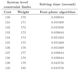
Furthermore, the following table contains the solving time of the presented algorithm with the exact solution for some problems in short scale, which can be solved using both exact models and the proposed algorithm. This indicates that in comparison to the exact model, the proposed algorithm solves dierent problems, eciently (Table 6). This feature is invalu-able, especially in solving large scale problems, which is a considerable issue in practice.
6. Conclusion
In this paper, a four phase algorithm is developed to solve RAP. This algorithm is compromised of one meta-heuristic and three eective heuristics, where the results indicate the eciency of the proposed algorithm to solve RAP, expeditiously. The main structure of this algorithm is that the best generated solution of each phase is considered the initial solution of the following step. Therefore, at each phase, the initial solution will be improved with high probability. As a new approach, rather than considering some constraints, such as weight and cost, we consider the redundancy strategy and number of components in each subsystem. On the other hand, we summarize the mathematical model more simply using common optimization tech-niques.
Future research areas on Relations (1) to (3), can be extended as per the following suggestions:
Applying other meta-heuristic algorithms rather than ACO in the rst phase of the proposed algo-rithm.
Utilizing extra heuristic phases to improve the gen-erated solution as much as possible in a reasonable time period.
Modeling the problem using various types of com-ponents in each subsystem, simultaneously.
Table 5. Solving time of the proposed algorithm. Solving time (second)
Periods Iteration 1 Iteration 2 Iteration 3 Iteration 4 Iteration 5 Iteration 6 Iteration 7 Iteration 8 1 0.859375 0.843750 0.843750 0.843750 0.859375 0.863281 0.855469 0.859375 2 0.855469 0.839844 0.851563 0.839844 0.855469 0.855469 0.882813 0.859375 3 0.855469 0.843750 0.847656 0.843750 0.855469 0.855469 0.859375 0.855469 4 0.855469 0.839844 0.843750 0.839844 0.859375 0.855469 0.859375 0.855469 5 0.855469 0.839844 0.843750 0.843750 0.855469 0.851563 0.859375 0.863281 6 0.855469 0.839844 0.839844 0.839844 0.855469 0.859375 0.859375 0.855469 7 0.847656 0.839844 0.839844 0.839844 0.855469 0.859375 0.859375 0.859375 8 0.859375 0.839844 0.839844 0.839844 0.855469 0.855469 0.855469 0.859375 9 0.855469 0.839844 0.839844 0.835938 0.855469 0.859375 0.859375 0.859375 10 0.855469 0.839844 0.835938 0.839844 0.847656 0.855469 0.855469 0.867188 11 0.855469 0.843750 0.839844 0.839844 0.859375 0.859375 0.859375 0.871094 12 0.855469 0.851563 0.843750 0.839844 0.859375 0.859375 0.855469 0.875000 13 0.867188 0.839844 0.839844 0.839844 0.855469 0.855469 0.855469 0.859375 14 0.851563 0.867188 0.839844 0.832031 0.855469 0.855469 0.859375 0.859375 15 0.875000 0.839844 0.839844 0.816406 0.867188 0.859375 0.859375 0.859375 16 0.859375 0.839844 0.839844 0.839844 0.871094 0.855469 0.843750 0.859375 17 0.855469 0.843750 0.835938 0.839844 0.871094 0.859375 0.859375 0.855469 18 0.855469 0.839844 0.839844 0.835938 0.859375 0.855469 0.859375 0.859375 19 0.859375 0.839844 0.839844 0.839844 0.855469 0.863281 0.859375 0.859375 20 0.867188 0.839844 0.839844 0.839844 0.859375 0.863281 0.855469 0.859375 Max 0.875000 0.867188 0.851563 0.843750 0.871094 0.863281 0.882813 0.875000 Min 0.847656 0.839844 0.835938 0.816406 0.847656 0.851563 0.843750 0.855469 Standard
deviation 0.005998 0.006475 0.003646 0.005846 0.005650 0.003206 0.006778 0.005085 Period Iteration 9 Iteration 10 Iteration 11 Iteration 12 Iteration 13 Iteration 14 Iteration 15
1 0.859375 0.859375 0.859375 0.859375 0.859375 0.859375 0.859375 2 0.859375 0.859375 0.855469 0.859375 0.859375 0.859375 0.859375 3 0.859375 0.859375 0.859375 0.859375 0.859375 0.859375 0.859375 4 0.859375 0.855469 0.867188 0.859375 0.859375 0.871094 0.855469 5 0.859375 0.851563 0.859375 0.859375 0.855469 0.859375 0.855469 6 0.855469 0.859375 0.875000 0.859375 0.855469 0.882813 0.859375 7 0.859375 0.859375 0.855469 0.855469 0.859375 0.859375 0.859375 8 0.855469 0.859375 0.859375 0.855469 0.859375 0.859375 0.859375 9 0.855469 0.843750 0.859375 0.867188 0.859375 0.855469 0.871094 10 0.859375 0.847656 0.859375 0.863281 0.855469 0.859375 0.855469 11 0.855469 0.859375 0.859375 0.871094 0.855469 0.855469 0.878906 12 0.859375 0.859375 0.855469 0.859375 0.859375 0.863281 0.859375 13 0.859375 0.859375 0.859375 0.859375 0.859375 0.859375 0.859375 14 0.863281 0.859375 0.859375 0.871094 0.855469 0.855469 0.859375 15 0.859375 0.859375 0.859375 0.859375 0.859375 0.859375 0.859375 16 0.882813 0.859375 0.855469 0.878906 0.855469 0.859375 0.859375 17 0.855469 0.855469 0.859375 0.855469 0.859375 0.859375 0.863281 18 0.859375 0.855469 0.863281 0.855469 0.859375 0.859375 0.859375 19 0.863281 0.871094 0.851563 0.859375 0.867188 0.855469 0.855469 20 0.859375 0.859375 0.847656 0.855469 0.855469 0.855469 0.859375 Max 0.882813 0.871094 0.875000 0.878906 0.867188 0.882813 0.878906 Min 0.855469 0.843750 0.847656 0.855469 0.855469 0.855469 0.855469 Standard
Table 6. Solving time for dierent problems using proposed algorithm.
System level
constraint limits Solving time (second) Cost Weight Four-phase algorithm
130 170 0.839844
131 171 0.855469
132 172 0.847656
133 173 0.839844
134 174 0.851563
135 175 0.855469
136 176 0.855469
137 177 0.839844
138 178 0.839844
139 179 0.843750
140 180 0.843750
References
1. Sadjadi, S.J. and Soltani, R. \An ecient
heuris-tic versus a robust hybrid meta-heurisheuris-tic for general framework of serial-parallel redundancy problem", Re-liability Engineering and System Safety, 94, pp. 1703-10 (2009).
2. Kuo, W. and Prasad, V.R. \An notated overview of
system-reliability optimization", IEEE Transactions on Reliability, 29(2), pp. 176-87 (2000).
3. Hsieh, Y.C., Chen, T.C. and Bricker, D.L. \Genetic
algorithm for reliability design problems", Microelec-tronics Reliability, 38, pp. 599-605 (1998).
4. Chern, M.S. \On the computational complexity of
reliability redundancy allocation in a series system", Operration Research Letter, 11, pp. 309-15 (1992).
5. Coit, D.W. and Smith, A.E. \Optimization approaches
to the redundancy allocation problem for series -prallel systems", Proceedings of the Fourth Industrial Engineering Research Conference (IERC) (1995).
6. Tillman, F.A., Hwang, C.L. and Kuo, W.
\Optimiza-tion techniques for systems reliability with redundancy - A review", IEEE Transactions on Reliability, 26, pp. 148-55 (1977).
7. Yokota, T., Gen, M. and Ida, K. \System reliability of optimization problems with several failure modes by genetic algorithm", Japanese Journal of Fuzzy Theory and Systems, 7(1), pp. 117-35 (1995).
8. Sung, C.S. and Cho, Y.K. \Reliability optimization of
a series system with multiple-choice and budget con-straints", European Journal of Operational Research, 127, pp. 159-71 (2000).
9. Ramirez-Marquez, J.E. and Coit, D.W. \A heuristic
for solving the redundancy allocation problem for multi-state series-parallel systems", Reliability Engi-neering and System Safety, 83, pp. 341-9 (2004).
10. Bris, R., Chatelet, E. and Yalaoui, F. \New method
to minimize the preventive maintenance cost of series-parallel systems", Reliability Engineering and System Safety, 82, pp. 247-55 (2003).
11. Yalaoui, A., Chu, C. and Chatelet, E. \Reliability al-location problem in series-parallel system", Reliability Engineering and System Safety, 90, pp. 55-61 (2005).
12. Ruan, N. and Sun, X. \An exact algorithm for cost
minimization in series reliability systems with multiple component choices", Applied Mathematics and Com-putaion, 181, pp. 732-41 (2006).
13. Nahas, N. and Nourelfath, M. \Ant system for reliabil-ity optimization of a series system with multiple-choice and budget constraints", Reliability Engineering and System Safety, 87, pp. 1-12 (2005).
14. Zhao, J.-H., Liu, Z. and Dao, M.-T. \Reliability
op-timization using multiobjective ant colony system ap-proaches", Reliability Engineering and System Safety, 92, pp. 109-20 (2007).
15. Kashtanov, V.A. \Controlled semi-markove processes
in modeling of the reliability and redundancy mainte-nance of queuing systems", Computer Modelling and New Technologies, 14, pp. 26-30 (2010).
16. Ahmadizar, F. and Soltanpanah, H. \Reliability
op-timization of a series system with multiple-choice and budget constraints using an ecient ant colony approach", Expert Systems with Applications, 38, pp. 3640-6 (2011).
17. Tavakkoli-Moghaddam, R., Safarib, J. and Sassani,
F. \Reliability optimization of series-parallel systems with a choice of redundancy strategies using a genetic algorithm", Reliability Engineering and System Safety, 93, pp. 550-6 (2008).
18. Dorigo, M., Maniezzo, V. and Colorni, A. \Positive
feedback as a search strategy", Technical Report (1991).
Biographies
Ali Ghafarian Salehi Nezhad is an MS degree student of Industrial Engineering at Sharif University of Technology, Tehran, Iran. His research interests include reliability optimization, developing heuristic al-gorithms, new product development, and facility layout problems, especially in the eld of robust optimization in uncertain environments. His MS thesis concentrates on reliability and robust optimization.
Abdolhamid Eshraghniaye Jahromi received his PhD degree in Industrial Engineering and Operations Research from the Polytechnic University of New York, USA, in 1992, and is currently Associate Professor in the Industrial Engineering Department at Sharif Uni-versity of Technology, Tehran, Iran. He has published various papers in the areas of component and system reliability, maintenance engineering, optimal policies
in inventory systems, and optimal topological design of power communication networks, as well as teach-ing courses in component reliability, system reliabil-ity, work methods management, work measurements, engineering economy, and operations research. His current research interests include reliability engineer-ing, productivity, quantitative methods, and methods engineering.
Mohammad Hassan Salmani is a PhD degree student of Industrial Engineering at Sharif University of Technology, Tehran, Iran. His research interests include Operational Research and Mathematical Pro-gramming, especially in the eld of robust
optimiza-tion. His PhD thesis concentrates on combinatorial optimization and he would like to develop an algo-rithm to solve more practical large scale problems, eciently.
Fereshte Ghasemi is an MS degree student of Indus-trial Engineering at Amirkabir University of Technol-ogy (Tehran Polytechnic), Iran. Her research interests include reliability, quality management, operational research, and new product development. Her MS thesis concentrates on New Product Development and system dynamics, and, currently, she is working in the Petrochemical Industry as a planning, project control, and cost control expert.