Sharif University of Technology
Scientia IranicaTransactions A: Civil Engineering www.scientiairanica.com
Shape optimization of concrete arch dams considering
stage construction
S. Pourbakhshian
a, M. Ghaemian
b;and A. Joghataie
ba. Department of Civil Engineering, Science and Research Branch, Islamic Azad University, Tehran, Iran. b. Department of Civil Engineering, Sharif University of Technology, Tehran, Iran.
Received 30 October 2013; received in revised form 14 June 2014; accepted 20 October 2014
KEYWORDS Arch dam;
Shape optimization; Stage construction; Simultaneous perturbation stochastic approximation; Cubic spline.
Abstract. This paper describes a methodology to develop the interface between a nite element software and optimization algorithm for optimization of concrete high arch dams. The objective function is the volume of the dam. The numbers of design variables are 31 including the thickness and upstream prole of crown cantilever, thickness of the left and right abutments, radius of curvature of water and air faces left and right by use of polynomial curve tting and cubic spline function. The constraint conditions are the geometric shape, stress, and the stability against sliding. Initially, a program is developed in MATLAB in order to generate the coordinates of nodes; then, nite element software ANSYS is taken for modeling the geometry of dam. Finally, the optimization technique is performed by Simultaneous Perturbation Stochastic Approximation algorithm. To include dead weight of dam body, stage construction is considered. The proposed method is applied successfully to an arch dam and good results are achieved. The results indicate that the concrete volume of the optimized dam is reduced by an average of 21%. Compared with the initial shape, the time of convergence in this method is very short and the method is fairly eective. It can be applied to practical engineering design.
© 2016 Sharif University of Technology. All rights reserved.
1. Introduction
The optimal shape is the best design for a structure subject to various constraints imposed by the restric-tions placed on the design. Shape optimization is the key step in the design of an arch dam.
The geometrical shape dened during the initial design phase is not always the best one from technical and economical points of view. The best shape should be dened by means of optimization studies, which employ a set of structural safety and minimal cost criteria [1]. Introduction to Optimum Design started from the late 1960's and several dierent researchers
*. Corresponding author. Tel.: +98 21 66164242
E-mail addresses: [email protected] (S. Pourbakhshian); [email protected] (M. Ghaemian)
continued it [2-22]. In recent years, many methods of optimization are being developed rapidly and much attention has been paid by several authors to the elds of concrete arch dam.
Sun et al. [23] established an optimization model for the shape design of arch dam by the use of cubic spline arch for the shape parameters, such as the coordinates of nodes, semi-center angle, and the thickness of arch abutment. The results indicated that the concrete volume of the arch dam optimized by the proposed cubic spline was less than the original design scheme optimized using parabolic shape. Li et al. [24] used the modied complex method which can search for the optimal solution directly, has no special request on the condition of the objective function and constraint function, and does not need to derivate during iteration pilot calculation. Fanelli [25] showed that the degrees of
freedom, which are strictly necessary to be considered in the shape optimization procedure of an arch dam, can be reduced by a judicious choice of basic model and design variables. Peng et al. [26] expressed that the optimization of arch dams is complex, because its objective function and constraint conditions appear non-linear and it applies a genetic algorithm with closure temperature eld for shape optimization of arch dams.
Tajalli et al. [27] used Bofang formulation for parabolic arch dam. The nite element analysis and op-timization procedure are implemented by commercial programs. The combination of Simultaneous Pertur-bation Stochastic Approximation (SPSA) and Particle Swarm Optimization (PSO) algorithm is introduced by Hamidian et al. [28] to nd the optimal shapes of arch dams. Akbari et al. [29] employed a new algorithm for geometry modeling of arch dams using Hermit cubic splines and the optimization problem solved via the Sequential Quadratic Programming (SQP) method. Takalloozadeh and Ghaemian [30] did the shape opti-mization of arch dams considering abutment stability with Particle Swarm Optimization (PSO) method.
The present study describes a method for shape optimization of double curvature concrete arch dam. In the optimization process, the objective function is volume of the concrete arch dam. Design variables of processing are the geometric shape parameters of the double curvature of arch dam and the constraint conditions are geometric shape, stress, and stability against sliding. The program basically consists of three parts that are described in the paper:
1. Generation of the coordinate of nodes by MATLAB code;
2. Call ANSYS batch le for analysis;
3. Optimization of the arch dams by SPSA algorithm according to the established load combination.
For optimization purposes, it is convenient to con-sider the eects of dam body dead weight and upstream hydrostatic pressures. To include dead weight of dam body, stage construction is considered. The proposed method is successfully applied to an arch dam, where good results are achieved. The results indicate that the concrete volume of the optimized arch dam is reduced by an average of 21%. Compared with the initial shape, the time of convergence in this method is very short and the method is fairly eective. It can be applied to practical engineering design.
2. Mathematical equation of arch dam design 2.1. Preliminary design
The main geometric parameters of the arch dam are shown in Table 1.
Table 1. The main geometric parameters.
K Arch number
EL Elevation
TC Thickness of the crown cantilever
TAL Left abutment thickness
TAR Right abutment thickness
USP Crown cantilever upstream prole DSP Crown cantilever downstream prole RLUS Radius of curvature of left water face
RRUS Radius of curvature of right water face
RLDS Radius of curvature of left air face
RRDS Radius of curvature of right air face
xeL Left abetment curve
xeR Right abetment curve
2.2. The geometric model of an arch dam The shape of an arch dam is of paramount importance in its ultimate behavior and eventually settles all design criteria. Variable curvature arch dams evolved to be economical in shape optimization studies [31].
These geometrical parameters can be dened as follows.
2.2.1. Crown cantilever shape
For denition of crown cantilever, two quadratic func-tions of vertical coordinates for water and air face are employed.
USP(Z) = a0+ a1Z + a2Z2; (1)
DSP(Z) = b0+ b1Z + b2Z2; (2)
in which Z is vertical coordinate; a0, a1, a2, and b0,
b1, b2 are the coecients, and extrude is the curved
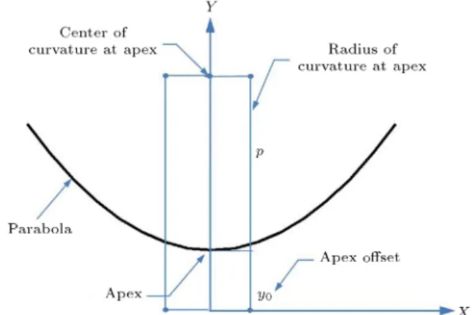
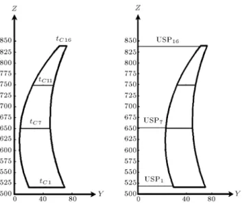
upstream surface of the horizontal arch elements. The intrados is the curved downstream surface of horizontal arch elements; USP and DSP are the crown cantilever U/S (upstream) and D/S (downstream) prole, respec-tively. In other words, USP is the horizontal distance between the extrados and the axis on a line normal to the extrados and the DSP is the horizontal distance between the intrados and the axis on a line normal to the intrados. In Figure 1, the shape of crown cantilever and layers at control elevations are shown.
2.2.2. Thickness of arch dam
In this paper, the variations of thicknesses of the verti-cal crown cantilever and the horizontal arch sections are taken to be the third-degree polynomials of the vertical coordinate. The thicknesses of the arch horizontal sections are calculated using the following equations:
tc(Z) = c0+ c1Z + c2Z2+ c3Z3; (3)
Figure 1. Cross section of crown cantilever.
tAR(Z) = e0+ e1Z + e2Z2+ e3Z3; (5)
in which tc(Z), tAL(Z), and tAR(Z) are the crown,
left, and right abutment thicknesses, respectively. Z is vertical coordinate and c0; :::; c3, d0; :::; d3, and e0; :::; e3
are the coecients. In this way, the downstream prole can be written in the following form:
DSP = USP + tc: (6)
2.2.3. Radius of curvature
The cubic spline is used to dene the radii of curvature of water and air faces. The number of horizontal arch layers is selected as 16 from the base to the crest elevation (Figure 1).
The radius of curvature R is specied at inter-polation points by R1, R7, R11, R16 (RLUS1, RLUS7,
RLUS11, RLUS16, RRUS1, RRUS7, RRUS11, RRUS16,
RLDS1, RLDS7, RLDS11, RLDS16, RRDS1, RRDS7,
RRDS11, RRDS16) as design variables. R is interpolated
at each level with the following cubic spline (Figure 2).
Figure 2. Cubic spline.
Given the following list of points:
a = x0< x1<; :::; < xn= b ! x 2 jxi; xi+1j !
(i = 0; 1; :::; n 1)
y0 y1 ; :::; yn: (7)
A cubic spline S(x) is a piecewise-dened function that satises the following conditions:
1. S(x) = Si(x) is a cubic polynomial on each
subinter-val:
[xi; xi+1] (i = 0; 1; :::; n 1); (8)
2. S(xi) = yi i = 0; 1; :::; n, (9)
S interpolates all the points.
3. S(x), S0(x), and S00(x) are continuous on [a; b] (S
is smooth).
So, the n cubic polynomial pieces can be written as:
Si(x)=ai+bi(x xi)+ci(x xi)2+ di(x xi)3;
i = 0; 1; :::; n 1; (10)
in which ai, bi, ci, and di represent 4n unknown
coecients. The following conditions are held for interpolation and continuity:
a) S(x) is continuous at discrete points:
Si(xi) = yi; i = 0; 1; :::; n 1; (11)
Si(xi+1) = yi+1; i = 0; 1; :::; n 1: (12)
b) Derivatives of S(x) at discrete points are: S0
i(xi+1) = Si+10 (xi+1) i = 0; 1; :::; n 2; (13)
S00
i(xi+1) = Si+100 (xi+1); i = 0; 1; :::; n 2: (14)
Based on conditions (a) and (b), the total number of equations is 4n 2. The expressions for the derivatives of Si can be written as:
Si(x)=ai+bi(x xi)+ci(x xi)2+di(x xi)3; (15)
S0
i(x) = bi+ 2ci(x xi) + 3di(x xi)2; (16)
S00
i(x) = 2ci+ 6di(x xi): (17)
If hi = xi+1 xi, then the spline conditions can be
written as follow (substitute Eqs. (11) to (14) into Eqs. (15) to (17)):
ai= yi; (18)
bi+ 2hici+ 3h2idi bi+1 = 0; (20)
2ci+ 6hidi 2ci+1= 0: (21)
The above equations can be written as a linear system for the 4n unknowns, i.e. a0, b0, c0, d0, a1, b1, c1, d1,...,
an 1, bn 1, cn 1, dn 1.
The denition of term mi is given in Eq. (22):
S00
i(xi); :::; Si00(xi) = 2ci or ci= mi=2: (22)
Considering mi as unknowns instead, we have
(substi-tute Eqs. (22) and (14) into Eq. (21)):
di = (mi+1 mi)=(6hi): (23)
Substitute Eqs. (11) and (12) into Eq. (19) in the following:
yi+ hibi+ h2ici+ h3idi= yi+1: (24)
Substituting ci and di from Eqs. (22) and (23) into
Eq. (21), the following is obtained: bi= yi+1h yi
i
hi
2mi hi
6 (mi+1 mi): From Eq. (13) we have:
bi+ 2hici+ 3h2idi= bi+1: (25)
Substitute Eqs. (22), (23) and (25) into Eq. (21): himi+ 2(hi+ hi+1)mi+1+ hi+1mi+2
= 6
yi+2 yi+1
hi+1
yi+1 yi
hi
: (26)
These are (n 1) linear equations for (n+1) unknowns, i.e. m0, m1, m2, . . . , mn, where mi= g00i(xi).
For taken together gives an (n+1)(n+1) system of equation as shown in Box I.
Figure 3. Parabola denition. 2.2.4. Horizontal arches
For denition of dam geometry in horizontal sections, parabolic conic functions are employed (Figure 3). The general equation of water and air face parabolas is:
8 > > > > > > < > > > > > > :
ax2+ bxy + cx2+ dx + ey + f = 0
= 4ac b2
< 0 hyperbola > 0 ellipse = 0 parabola
(28a)
Corresponding coecients of general conic function shall be as follows:
8 > > > > > > > > < > > > > > > > > :
a = 1 b = 0
c = 0 ) y = y0+(x x0) 2 2p
d = 2x0
e = 2p f = x2
0+ 2py0
(28b)
In Figure 3, some related details and geometric param-eters, used to dene a general horizontal parabolic arch, are shown. Each parabola is dened by the position of its apex (y0) and its radius of curvature at the apex.
In water face, y0=USP, and the radius of curvature are
2 6 6 6 6 6 6 6 6 6 4
1 0 0 0
h0 2(h0+ h1) h10 0
0 h1 2(h1+ h2)h2 0
0 0 h22(h2+ h3) h3 0
... ... ... ... ...
0 hn 2 2(hn 2+ hn 1) hn 1
0 0 0 1
3 7 7 7 7 7 7 7 7 7 5 2 6 6 6 6 6 6 6 4 m0 m1 m2 m3 ... mn 3 7 7 7 7 7 7 7 5 2 6 6 6 6 6 6 6 6 6 4 0
y2 y1
h1
y1 y0
h0
y3 y2
h1
y2 y1
h1
y4 y3
h1
y3 y2
h2
: :
yn yn 1
hn 1
yn 1 yn 2
hn 1
3 7 7 7 7 7 7 7 7 7 5
= 6 (27)
If m0= 0 , mn = 0, the above equation system will be reduced to (n + 1) (n + 1) system.
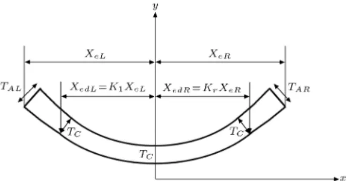
Figure 4. A horizontal arch of the dam body.
RLUS and RRUS. In air face, y0= DSP, and the radius
of curvature are RLDS and RRDS. Again, the radii of curvature at apex point are dened by spline. The axes of three parabolas are coincident and are positioned on dam reference plane.
To dene the horizontal section, two parabolic curves are dened in the left and right sides of Figure 4. This is done in order to model an unsymmetrical arch dam. Each side is divided into two segments: constant thickness and variable thickness. The thickness of the dam in horizontal section is constant in the rst segment and increases by parabolic function in the second one [32]. Coecients kr and kl determine
portion of the length of arch with constant thickness in the right and left banks. In this paper, krand klare
equal to 2/3. 8 > > > > > > > > > > > > > < > > > > > > > > > > > > > :
For the right half TaR(x) = TC+(x xedR)
2(TAR TC)2 (xeR xedR)2
xedR< x < xeR
TaR= TC x < xedR
For the left half
TaL(x) = TC+(x xedL)
2(TAL TC)2 (xeL xedL)2
xedL< x < xeL
TaL= TC x < xedL
(29)
xedL and xedR are lengths of segments with constant
thicknesses in the left and right banks, respectively (Figure 4).
Dierence in the x coordinates of the upstream surface corresponds to 25 meters (x).
The number of horizontal arch layers is selected as 16 from the base to the crest elevation. This can be selected based on dam elevation for each layer. In Table 1, the basic input parameters for denition of crown cantilever and horizontal arches are included. The x coordinate of the vertical middle line can be calculated from the x coordinate of the upstream (xeu)
and downstream surface (xid), which can be written
as:
xeu+ xid
2 : (30)
2.2.5. Programming and implementation of 3D model and loadings
According to the above formula, a MATLAB program for geometrical design of arch dams was written so that Finite element model was developed in the APDL programming language of the ANSYS code. In -nite element modeling of the arch dam, geometry is considered as doubled curvature arch dam. In the nite element model of an arch dam, 1580 eight-node elements in the foundation and 180 twenty-eight-node elements in the dam body are used. Each node has three degrees of freedom: translations in the nodal X, Y and Z directions. Two layers of elements were set along thickness of the dam. The nite element model of the dam is developed so that it includes the foundation. As it is shown in Figure 4, the length and width of the foundation along the global X and Y axes are taken to be 1650 m. For the 3D arch dam analysis, mass concrete and rock were assumed to be homogeneous with linear elastic materials. The modulus of elasticity of mass concrete was taken as 28 GPa and that of the foundation rock as 9 GPa. The Poisson's ratios of mass concrete and rock were taken as 0.18 and 0.25, respectively. Mass density of the concrete was chosen as 2400 kg/m3and no gravity
load was applied on the foundation rock. Concrete and rock were assumed to be homogeneous and isotropic materials. As the foundation is assumed as massless, only the eects of foundation exibility are considered in the analysis. For the boundary conditions in the nite element model of the dam, all degrees of freedom are xed at the outside surfaces of the foundation.
Figure 5 illustrates the dam, foundation, and reservoir nite element model. The usual static cases include the eects of silt and tail water pressures and temperature (either summer or winter), while for optimization purposes, it is convenient to exclude all these eects and merely consider the eects of dam body dead weight and upstream hydrostatic pressures. In this research, two basic loading cases, as follows, have been considered for the optimization procedure:
1. SU1 (the rst usual static load combination) or self-weight;
2. SUN1 (the rst unusual static unusual load
com-Figure 5. Three-dimensional shape of an arch dam with foundation.
Table 2. Load combinations used for presenting the analyses results.
Load Single load parts Factor of safety Load
combination number
Dead weight
Normal water
pressure Tension Compression combination
SU1 p p 2 3 Static usual
SUN1 p - 1.5 2 Static unusual
Figure 6. Construction stages.
bination) or self-weight and upstream hydrostatic pressures.
Two dierent load combinations are listed in Table 2.
As the self-weight considered by staged construc-tion method in which dead load is applied in several stages.
As shown in Figure 6, self-weight simulation is carried out in 8 stages. Indeed, it is assumed that each stage corresponds to a lift of concrete. The lift height is taken equal to the vertical distance between two consecutive horizontal arches enclosing one row of nite elements in the model. The element birth option of the ANSYS program is adequately utilized to resemble addition of nite elements i.e. concrete lifts to the whole model. The birth time of the elements of any specic lift corresponds to the placement time of that lift. The placement time is just a ctitious number and does not intend to resemble the real practical situation. It is worth to mention that the whole concrete of each lift (one stage) is assumed to be placed simultaneously.
3. The optimization method of arch dam shape Shape optimization aims to minimize consumed con-crete volume while enhancing safety criteria. The shape optimization problem is to nd the design vari-able X while minimizing the objective function F (x) under the constraint functions hj(X) and gj(X) that
can be stated mathematically as: Find X = [X1; X2; :::; Xn]T;
ai X bi (i = 1; 2; :::; n):
To minimize F (x)
hj(X) = 0 (j = 1; 2; :::; p);
gk(X) 0 (k = 1; 2; :::; m): (31)
The subscripts p, m, and n denote the number of equality constraints, behavioral constraints, and design variables, respectively, where ai and bi are allowable
lower and upper limits of the design variables, which are introduced to deal with various requirements. 3.1. Design variables
Shape optimization can be improved by increasing the number of design variables, but it raises the cost of calculations. According to the geometrical model of arch dams described before in the paper, the design variables can be selected as: 31 design variables, which will be used in the process of optimization, as shown in Table 3.
Crown cantilever design variables are shown in Figure 7.
3.2. Objective function
The purpose of optimization is to choose proper geometric shape of arch dam to make the project cost minimal on the premise of meeting the needs of Table 3. Design variables.
Thickness Radius USP
tC1 tAL1 tAR1 RLUS1 RRUS1 RLDS1 RRDS1 USP1
tC7 tAL7 tAR7 RLUS7 RRUS7 RLDS7 RRDS7 USP7
tC11 tAL11 tAR11 RLUS11 RRUS11 RLDS11 RRDS11 USP16
Figure 7. Crown cantilever design variables.
strength and stability. Generally, the cost of arch dam is mainly dependent upon the volume of dam body concrete. So, the objective function is the dam body volume.
3.3. Constraint functions
In shape optimization of concrete arch dams, the fol-lowing three types of constraint sets should be satised, as required by the demands of design and construction:
1. Geometrical constraints;
2. Stress constraints;
3. Stability constraints.
3.3.1. Geometrical constraints set
Thickness of horizontal arch: The thickness of crown cantilever decreases from base to the dam crest.
TCi+1 < TCi! TTCi+1
Ci 1 0 (i = 0; 1; :::; n): (32)
For dierent elevations, the crown cantilever thickness is lower than abutment thickness.
TCi < TARi ! TTCi
ARi 1 0 (i = 0; 1; :::; n); (33)
TCi<TALi! TTCi
ALi 1 0 (i=0; 1; :::; n): (34)
Slope of overhang in upstream and downstream of arch dam: To facilitate construction, the maximum slope of overhang at the upstream and downstream faces should be controlled as follows (Figure 8).
Below tangent points, the angles of tangents are negative and above it, they are positive. The plotting steps should be increased to avoid gap in curves of the upper and lower parts.
U
max Ualw; (35)
Figure 8. The slope of overhang in upstream and downstream of arch dam.
D
max Dalw; (36)
where U
max and Dmax are the allowable maximal
over-hang slopes of the upstream and downstream surfaces, and U
alw and alwD are the allowable maximal overhang
slopes, respectively.
Crown cantilever prole: Below tangent points, the angles of tangents are negative and above it, they are positive. The plotting steps should be increased to avoid gap in curves of the upper and lower parts. Crown cantilever upstream prole:
USPi+1< USPi! USPUSPi+1
i 1 0
(i = 0; 1; :::; ntangant point; :::; n); (37)
USPi< USPi+1! USPUSPi
i+1 1 0
(i = ntangant point; :::; n): (38)
Crown cantilever downstream prole: DSPi+1< DSPi! DSPDSPi+1
i 1 0
(i = 0; 1; :::; ntangant point; :::; n); (39)
DSPi< DSPi+1! DSPDSPi
i+1 1 0
(i = ntangant point; :::; n): (40)
Location of the tangent point: As shown in Figure 9, the maximum distance between crest and tangent point is 0.6 H [33].
Figure 9. Location of the tangent point. HTangant point<HTangant pointmax
! HTangant point HTangant pointmax
1 0: (42) Radius of curvature. The most important geomet-ric constraints are those that prevent intersection of upstream and downstream faces as:
RLDSi < RLUSi! RRLDSi
LUSi 1 0
(i = 0; 1; :::; n); (43)
RRDSi < RRUSi! RRRDSi
RUSi 1 0
(i = 0; 1; :::; n): (44)
The variation of radius at crown cantilever along with height of dam should be satisfactory to some kind of nonlinear variation rule.
RLUSi< RLUSi+1 ! RRLUSi
LUSi+1 1 0
(i = 0; 1; :::; n); (45)
RRUSi< RRUSi+1 ! RRRUSi
RUSi+1 1 0
(i = 0; 1; :::; n); (46)
RRDSi <RRDSi+1 !RRRDSi
RDSi+1 1 0
(i = 0; 1; :::; n); (47)
where RRUSi and RRDSiare radius of curvatures at the
upstream and downstream faces of the dam in the ith layer in z direction.
3.3.2. Stress constraints
Stress constraints are used to control stress distribution in the structure. Under dierent loads imposed on arch dam, the maximum stress is less than the allowable stress. In this study, the behavior constraints are dened to prevent failure of each element (i) of arch dam under specied safety factor (sf). For this purpose, the failure criterion of concrete of Willam and Warnke [32] due to multiaxial stress state is employed as follows:
f fc
s sf !
f fc
s
sf 0 (i = 0; 1; :::; ne); (48) where (f) is a function of the principal stress state (1 2 3) and (s) is failure surface expressed
in terms of principal stresses, uniaxial compressive strength of concrete (fc), uniaxial tensile strength
of concrete (ft), and biaxial compressive strength of
concrete (fcb). Table 4 shows the four principal stress
states by which the failure of concrete is categorized into four domains. In each domain, independent functions describe (f) and the failure surface (s). The details of failure criterion can be found in Willam and Warnke and the theory reference of ANSYS.
The angle of similarity () describes the relative magnitudes of the principal stresses as:
cos =p 21 2 3
2 [(1 2)2+(2+3)2+(3 1)2]1=2
: (49) The parameters (r1) and (r2) represent the failure
surface of all stress states with ( = 0) and ( = 60),
respectively, and they are functions of principal stresses and concrete strengths. The parameters (r1) and (r2)
and the angle () are shown in Figure 10.
Therefore, Eq. (40) must be checked for the center of all dam elements (ne) with safety factor that is
chosen as sf = 1. If it is satised, there is no crack or crush. Otherwise, the material will crack if any principal stress is tensile, while crushing will occur if all principal stresses are compressive.
Figure 10. Failure surface in the compression-compression-compression Regime.
Table 4. The equation of Willam and Warnke.
Domain (f; s)
Compression f =p1 15
(1 2)2+ (2 3)2+ (3 1)21=2
Compression
Compression s = 2r2(r22 r21) cos +r2(2r1 r2)[4(r22 r21) cos2+5r21 4r1r2]1=2
4(r2
2 r12) cos2+(r2 2r1)2
Tension f =p1
15
(2)2+ (2 3)2+ 321=2
Compression
Compression s =1 1
ft
2p
2(p22 p21) cos +p2(2p1 p2)[4(p22 p21) cos2+5p21 4p1p2]1=2
4(p2
2 p21) cos2+(p2 2p1)2
Tension f = i; i = 1; 2
Tension
Compression s =
ft
fc(1 +
3
fc)
Tension f = i, i = 1; 2; 3
Tension
Tension s =
ft
fc
3.3.3. Stability constraints
Central angle of the arch: In this paper, constraints ensuring the sliding stability of the dam may be expressed by central angle of the arch.
1 90U 0; 110U 1 0; (50)
1 90D 0; 110D 1 0; (51)
where () is the sum of central angles at the right and the left archs, and 90 U 110, 90 D 110.
Overturning: To verify the overall overturning sta-bility of crown cantilever arch dam monoliths:
USP1< Ybar! USPY 1
bar 1 0: (52)
4. Optimization algorithm
The Simultaneous Perturbation Stochastic Approxi-mation (SPSA) has recently attracted considerable attention in areas, such as statistical parameter esti-mation, feedback control, simulation-based optimiza-tion, signal and image processing, and experimental design. However, the SPSA has not been tested yet for structural optimization and this is the rst study employed for the purpose. The promising feature of the SPSA optimization algorithm is that it requires only two structural analyses in each cycle of optimiza-tion process, regardless of the optimizaoptimiza-tion problem dimensions. This attribute can drastically reduce the computational cost of the optimization, particularly in problems with a number of variables to be optimized. The following step-by-step summary shows the process of SPSA in arch dam optimization:
Step 1. Initialization and coecient selection. Set
counter index k = 0. Pick initial guess and non-negative coecients a, c, A, , and in the SPSA gain sequences ak = a=(A + k + 1) and ck =
c=(k+1). The choice of gain sequences (a
kand ck) is
critical to performance of SPSA. Spall provides some guidance on picking these coecients in a practically eective manner;
Step 2. Generation of the simultaneous perturbation vector. Generate an nv dimensional random
per-turbation vector k by Monte Carlo, where each of
the nv components of k is independently generated
from a zero mean probability distribution satisfying some conditions. A simple and theoretically valid choice for each component of k is using a Bernoulli
1 distribution with probability of 1/2 for each 1 outcome. Note that uniform and normal random variables are not allowed for the element in k by
the SPSA regularity conditions;
Step 3. Fitness function evaluations. Obtain two measurements of the tness function f(0) based on the simultaneous perturbation around the current design vector ^xk : f(^xk + ckk) and f(^xk ckk)
with the ck and k from Steps 1 and 2;
Step 4. Gradient approximation. Generate the si-multaneous perturbation approximation with the un-known accurate gradient G(^xk):
Gk(^xk) = cGk(^xk)=f(^xk+ ckk) f(^x2c k ckk) k
2 6 6 6 4
1 k1
1 k2
... 1
knv
3 7 7 7
5; (53)
Step 5. Updating ^x estimate. Use the standard Stochastic Approximation (SA) to update ^xkto a new
value ^xk+1:
^xk+1= ^xk akGck(^xk); (54)
Step 6. Iteration or termination. Return to Step 2 with k + 1 replacing k. Terminate the algorithm if the Maximum Number of Iterations (MNI) has been reached [28]. The ow chart of SPSA algorithm for the arch dam optimization problem can be shown in Figure 11.
5. Result
The optimization process of arch dam according to the above methodology converged after 1000 iterations.
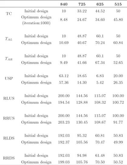
Figure 12 shows the evolution of crown cantilever shape. The initial and optimum values of shape design variables are given in Table 5 (all dimensions are in meters). As can be seen, the volume of the dam body dened by the present optimization is 1057550 m3less
than the initial volume, i.e. 21% less. Figure 11. The owchart of SPSA algorithm. Table 5. Initial and optimum values of shape design variables.
840 725 625 515
TC Initial design 10 33.22 44.52 50
Optimum design
(iteration:1000) 8.48 24.67 34.60 45.80
TAL Initial design 10 48.87 60.1 50
Optimum design 10.69 40.67 70.24 60.84
TAR Initial design 10 48.87 60.1 50
Optimum design 9.49 41.66 67.34 52.65
USP Initial design 63.12 18.65 6.83 20.00 Optimum design 57.36 14.30 5.42 26.35
RLUS Initial design 200.00 144.56 115.07 100.00 Optimum design 194.54 128.88 108.32 100.72
RRUS Initial design 200.00 144.56 115.07 100.00 Optimum design 203.23 130.45 108.67 91.77
RLDS Initial design 192.03 95.32 60.81 50.83 Optimum design 192.37 105.56 70.47 49.99
RRDS Initial design 192.03 94.98 61.48 50.83 Optimum design 199.03 105.76 70.50 50.52
Figure 12. Shapes of crown cantilever at dierent numbers of iteration. The dierence between the initial and optimum
design shapes can be seen in Figure 13. It is observed that the optimal design is thinner than the initial design and slope of overhang in upstream and down-stream of surfaces in the optimum design are smaller than those of the initial design, which are benets for construction [34].
The boldness coecient in Table 6 is calculated by Lombardi's formula, as follows:
Boldness coecient=(Height of dam)volumeMid surface area2 : (55) The boldness coecients for the initial and optimum designs are shown in Table 6. The boldness coecient for the optimum design is higher than that for the initial design.
The principal stresses for two load cases are shown in Figure 14 and Table 7. The position of maximum tensile stress is found close to the one third of dam height. The maximum tensile stresses are obtained for the U/S face in two cases SUN1 and SU1. For the case of SUN1, the maximum compression stress is observed in the U/S face and for the case the SU1, it is obtained
Figure 14. Principal stresses 1 and 3 in the initial and optimum design shapes for usual load combination (SU) and
Table 6. Boldness coecients for the initial and optimum designs. Lombardi boldness coecient ()
Design Height (m) Volume (m3) Mid surface area (m2)
Initial design 325 4.924.850 137314 11.78
Optimum design 325 3.863.840 137972 15.16
Table 7. Summary of the results of the models.
US DS
Maximum tension
Maximum compression
Maximum tension
Maximum compression
Initial design SUN1 1.72 -12.5 0.77 -4.26
SU1 4.3 -7.43 2.12 -8.99
Optimum design SUN1 1.85 -13 1.5 -4.4
SU1 6.12 -9.9 3.3 -10.9
Figure 15. Convergence rate of the dam body volume. The values of stresses for the optimum design are bigger than those for the initial design.
Convergence rate of the objective function in the optimization process is shown in Figure 15.
After performing the optimization process, the dam volume decreased by 21% in comparison with that in the initial design.
6. Conclusion
This paper employs a methodology to develop the inter-face between a nite element method and optimization algorithm for shape optimization of double curvature concrete arch dam.
In order to create the geometry of arch dams, a new algorithm is proposed in MATLAB. This algo-rithm is able to model the dierent shapes of an arch dam. The nite element of software ANSYS is taken for modeling the geometry of an arch dam used to consider the eects of dam body dead weight and upstream hydrostatic pressures. The following conclusions, some of which are important, are drawn from the present work:
It is concluded that SPSA can be eectively used in the shape optimization of arch dams;
Arch dam is a massive structure and therefore, its construction is staged into a step by step procedure. If the dead load is applied to the dam all at once, without taking into account the fact that horizontal load transfer cannot occur before the dam is complete, ctitious stresses will be indicated. By considering stage construction, there have been longer optimization process and lower optimum volume;
The maximum tensile stresses are obtained for the U/S face in two cases SUN1 and SU1. For the case of SUN1, the maximum compression stress is observed in the U/S face and for the case of SU1, it is obtained in the D/S case. After the shape optimization of the arch dam, the dam body volume is reduced by 21%. References
1. Grigorov, S., Tasev, S., Tzenkov, A., Fanelli, M. and Gunn, R. \Arch dam shape optimization procedure accounting for dam seismic response", Proceedings of the 11th National Congress on Theoretical and Applied Mechanics (2009).
2. Fialho, J.F.L. \Leading principles for the design of arch dams", A New Method of Tracing and Dimensioning, LNEC, Lisbon, Portugal (1955).
3. Seram, J.L. \New shapes for arch dams", Civil Engineering, ASCE, 36(2) (1966).
4. Rajan, M.K.S., Shell Theory Approach for Optimiza-tion of Arch Dam Shapes, University of California, Berkeley (1968).
5. Sharpe, R. \The optimum design of arch dams", Pro-ceedings of the ICE - Civil Engineering, Supplementary Volume, pp. 73-98 (1969).
6. Ricketts, R.E. and Zienkiewicz, O.C. \Shape opti-mization of concrete dams", Criteria and Assumptions for Numerical Analysis of Dams, Quadrant Press, Swansea, London, UK, pp. 1179-1206 (1975).
7. Mohr, G.A. \Design of shell shape using nite ele-ments", Computers & Structures, 10(5), pp. 745-749 (1979).
8. Sharma, R. \Optimal conguration of arch dams", Ph.D. Thesis, Indian Institute of Technology, Kanpur (1983).
9. Rahim, A.S. \Optimum shape of an arch dam for static loads", MEng Thesis, Asian Institute of Technology, Bangkok (1983).
10. Wasserman, K. \Three dimensional shape optimiza-tion of arch dams with prescribed shape funcoptimiza-tion", Journal of Structural Mechanics, 11(4), pp. 465-489 (1984)
11. Li, Y. and Bofang, Z. \The optimum design of arch dams and the curve of arch thickness", Journal of Hydraulic Engineering, CNKI (1985).
12. Bofang, Z. \Shape optimization of arch dams", Int. Water Power Dam Construct., 39(3) pp. 43-51 (1987).
13. Samy, M.S. and Wieland, M. \Shape optimization of arch dams for static and dynamic loads", in Pro-ceedings of International Workshop on Arch Dams, Coimbra (1987).
14. Yao, T.M. and Choi, K.K. \Shape optimal design of an arch dam", Journal of Structural Engineering, ASCE, 115(9), pp. 2401-2405 (1989).
15. Guohua, L. and Shuyu, W. \Optimum design of con-crete arch dam", Proc. Int. Concon-crete Conf., Tehran, pp. 444-452 (1990).
16. Sim~oes, L.M.C., Lapa, J.A.M. and Negrao, J. \Search for arch dams with optimal shape", In Arch Dams, pp. 99-114 (1990).
17. Bofang, Z. \Optimum design of arch dams", Dam Eng. I, 2, pp. 131-145 (1990).
18. Bofang, Z., Rao, B., Jia, J. and Li, Y. \Shape optimization of arch dams for static and dynamic loads", J. Struct. Eng., ASCE, 118(11), pp. 2996-3015 (1992).
19. Bofang, Z., Jinsheng, J., Rao, B. and Yisheng, L. \Mathematical models for shape optimization of arch dams", Journal of Hydraulic Engineering (1992).
20. Fanelli, A., Fanelli, M. and Salvaneschi, P. \A neural network approach to the denition of near optimal arch dam shape", Dam Eng., 4(2), pp. 123-140 (1993).
21. Guohua, L. and Shuyu, W. \Methods and applications of arch dam optimization", Chinese Journal of Com-putational Mechanics (1994).
22. Yisheng, L. \The optimum type of ring for arch dam", Journal of Hydraulic Engineering (1996).
23. Sun, L.S., Zhang, W.H. and Guo, X.W. \Shape optimization of arch dams based on accelerated micro
genetic algorithm", Journal of Hohai University: Nat-ural Sciences, 36(6), pp. 758-762 (2008).
24. Li, S., Ding, L., Zhao, L. and Zhou, W. \Optimization design of arch dam shape with modied complex method", Advances in Engineering Software, 40(9), pp. 804-808 (2009).
25. Fanelli, A. \Some remark on shape optimization of arch dams", Mathematical Modeling in Civil Engineer-ing, 5 (2009).
26. Peng, H., Yao, W. and Huang, P. \The application of genetic algorithm to closure temperature elds and shape optimization of Jinping high arch dam", In 2010 Sixth International Conference on Natural Computation, 5, pp. 2489-2493 (2010).
27. Tajalli, F., Ahmadi, M.T. and Moharrami, H. \A shape optimization algorithm for seismic design of a concrete arch dam. Dam Engineering", Dam Engineer-ing, 18(2) (2007).
28. Seyedpoor, S.M., Salajegheh, J., Salajegheh, E. and Gholizadeh, S. \Optimal design of arch dams subjected to earthquake loading by a combination of simul-taneous perturbation stochastic approximation and particle swarm algorithms", Applied Soft Computing, 11(1), pp. 39-48 (2011).
29. Akbari, J., Ahmadi, M.T. and Moharrami, H. \Ad-vances in concrete arch dams shape optimization", Applied Mathematical Modeling, 35(7), pp. 3316-3333 (2011).
30. Takalloozadeh, M. and Ghaemian, M. \Shape op-timization of concrete arch dams considering abut-ment stability", Scientia Iranica, 21(4), pp. 1297-1308 (2014).
31. Abraham, S. and Narayanan, K.V. \Denition of geometry of variable radius arch dam with degree of polynomial in the 3D nite element analysis", In Proceedings of the 10th WSEAS (World Scientic and Engineering Academy and Society) International Con-ference on Mathematical and Computational Methods in Science and Engineering, pp. 133-136 (2008).
32. Hollerbuhl, L. "Crack propagation simulations for the Koelnbrein-Dam 1978" [Simulation der Schadigung der Kolnbreintalsperre wahrend des Ersteinstaus 1978], M.S. Thesis, Bauhaus-Universitat Weimar, German (2005).
33. Boggs, H.L., Guide for Preliminary Design of Arch Dams, US Department of the Interior, Bureau of Reclamation, 36 (1966).
34. Zhang, X.-f., Li, S.-y. and Chen, Y.-l. \Optimization of geometric shape of Xiamen arch dam", Advances in Engineering Software, 40(2), pp. 105-109 (2009).
Biographies
Somayyeh Pourbakhshian is a PhD degree can-didate in Civil Engineering Department, Science and Research Branch, Islamic Azad University, Tehran,
Iran. Her research interests are mathematical methods in optimization, shape and topology optimization of structures, and sensitivity analysis. In recent years, she has been working on shape optimization of concrete dam.
Mohsen Ghaemian is Professor in Civil Engineer-ing Department at Sharif University of Technology, Tehran, Iran. His current research activities include dynamic responses of gravity and arch dams, dam
reservoir interaction eects, seismic response of dams due to non-uniform excitations, and nonlinear behavior of concrete dams.
Abdolreza Joghataie is Faculty Member in Civil Engineering Department at Sharif University of Tech-nology, Tehran, Iran. His research interests include application of neural networks in dierent areas of structural engineering, including nonlinear dynamic analysis of dams.