ISSN: 2252-8938, DOI: 10.11591/ijai.v9.i1.pp25-32 25
Development of option c measurement and verification model
using hybrid artificial neural network-cross validation
technique to quantify saving
Wan Nazirah Wan Md Adnan1, Nofri Yenita Dahlan2, Ismail Musirin3
1Faculty of Engineering and Life Sciences, Universiti Selangor, Bestari Jaya, Selangor, Malaysia
1,2,3Faculty of Electrical Engineering, Universiti Teknologi MARA, Shah Alam, Selangor, Malaysia
Article Info ABSTRACT
Article history: Received Nov 1, 2019 Revised Jan 10, 2020 Accepted Jan 23, 2020
This paper aims to develop a hybrid artificial neural network for Option C Measurement and Verification model to predict monthly building energy consumption. In this work, baseline energy model development using artificial neural networks embedded with artificial bee colony optimization and cross validation technique for a small dataset were considered. Artificial bee colony optimization with coefficient of correlation fitness function was used in optimizing the neural network training process and selecting the optimal values of initial weights and biases. Working days, class days and cooling degree days were used as input meanwhile monthly electricity consumption as an output of artificial neural network. The results indicated that this hybrid artificial neural network model provided better prediction results compared to the other model. The best model with the highest value of coefficient of correlation was selected as the baseline model hence is used to determine the saving.
Keywords:
Artificial Bee Colony Artificial Neural Network Cross Validation
Energy Saving
Measurement & Verification
This is an open access article under the CC BY-SA license.
Corresponding Author: Wan Nazirah Wan Md Adnan,
Faculty of Engineering and Life Sciences, Universiti Selangor,
Bestari Jaya, Selangor, Malaysia. Email: [email protected]
1. INTRODUCTION
In recent years, measurement and verification (M&V) has become the popular method in determining energy saving. M&V is the process of using measurements to reliably determine actual savings created in relative to the baseline energy. This process is important in energy saving field in order to quantifying saving. The M&V process involves modeling, metering and sampling activities which create uncertainties in reporting of energy savings. It is important to precisely consider the accuracy and develop an accurate M&V methodology [1-2]. In M&V, the development of a baseline energy model is one of the important steps to determine the relationship between energy consumption and independent input variables. Thus, the baseline energy model was used to develop and estimate the adjusted baseline energy pattern hence to determine the savings.
There are several established protocols and guidelines for performing M&V of energy savings. Among all the guidelines, International Performance Measurement and Verification Protocol (IPMVP) is the most prominent and widely used M&V protocol. IPMVP is a support document clearly describes the common practice in measuring, computing and reporting savings achieved by energy or water efficiency projects at end user facilities. It presents M&V principles, IPMVP framework and explanations on common
M&V issues. IPMVP provides four measurement options to evaluate the saving [21] according to their area of application, Option A, B, C and D where Option A: Key Parameter Measurement, Option B: All Parameter Measurements, Option C: Whole Facility and Option D: Calibrated Simulation [3].
Recently, a study of the literature relating to the M&V has become popular all around the world. One of the initiatives was the study of energy and demand impact of the steam feed pump refurbishment and high-pressure turbine re-blade in coal fired power station aimed to increase efficiency in South Africa [4]. Meanwhile in Brazil, M&V concept was applied to evaluate energy efficiency project by replacing electric shower with solar water heating system [5]. In China, [6] reported that energy saving can be generated from power line transformation project. Recent study by [7-8] involved a groups of building in United States to study the impact of building retrofitting projects to energy consumption as well as energy saving. A number of authors from Malaysia have applied M&V to study the impact of energy saving in the commercial building as well as educational building [9-10]. Most of the widely used M&V application were energy efficiency lighting retrofit projects to improve the efficiency of the lighting system and to reduce the energy consumption [11-14]. According to IPMVP, the baseline energy development has been identified as one of the important and crucial steps in M&V. Key aspects in developing the baseline energy resulting in reporting energy savings are accuracy and uncertainty [3]. To date, mathematical model using linear regression is the most common method used in formulating the baseline energy model [10, 15]. Nonetheless, linear regression only suitable for linear relationship and may contribute large error for non-linear data.
Artificial Neural Networks (ANN) has been applied in several works to replace the linear regression method. ANN is one of the popular techniques for forecasting that imitates the operation of human brain. It has been used to solve various engineering problems [16-19]. In order to increase the performance of ANN model, hybridization of ANN with various optimization techniques to automatically find the optimum ANN parameters as opposed to the trial and error technique were introduced by some researchers. By doing this will lead to a better ANN performance accuracy and save time for experimenting. Optimization techniques is one of an artificial intelligence method that have been widely used by researchers [20-21]. To get the best result, large training data is needed as ANN learns from examples. When large data set are easily available, there is no problem to split the data into training, validation, and testing sets in ANN. However, there are some situations where the measured data are very limited, expensive or difficult to find. In such cases, the allocation of the available data to train, valid, and test is the main challenge to build an accurate ANN prediction model. The ANN model is sensitive towards the inputs and outputs data, where fewer number of inputs and outputs data may reduce its accuracy. Too small data may not be able to train the network properly and may not be able to evaluate the network performance accurately [22].
Option C data were derived from the monthly utility bills and usually, only a small dataset is available. Therefore, the available data were insufficient to train the network and predict the energy consumption. In view of the above mentioned facts, several sampling techniques were studied to increase the accuracy of small data and the most common techniques used is cross-validation (CV) [22-24]. This study focuses on the development of Option C baseline energy model and the hybridizetion of ANN with ABC optimization. Cross Validation (CV) is integrated with this hybrid artificial neural network (HANN) to get a better accuracy of ANN prediction. This method may avoid any overfitting of the data. Overfitting creates the network to memorize training patterns, but they cannot generalize well to new data (testing set) and generates poor accuracy. This chapter is organised as follows: Section 2 briefly explains the proposed Option C M&V HANN model including baseline model development and saving calculations. Section 3 discusses the result of the proposed methods. Finally, Section 4 provides the conclusion.
2. RESEARCH METHOD
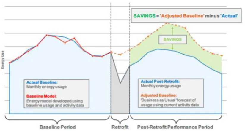
As savings cannot be directly measured in M&V, the savings can be determined by comparing the measured energy used before and after ECM implementation. Figure 1 shows the energy use during baseline period and post retrofit period. The baseline period is the time before the retrofit installation while the post retrofit period is the interval after installing the ECM. According to the IPMVP, to properly calculate savings using M&V, the baseline energy model is first developed to determine the relationship between energy use and independent variables using regression analysis. The independent variable is a parameter that is expected to change regularly and have impact on energy use. To fairly compare the energy use before and after the ECM implementation, the variable conditions in baseline and post retrofit period must be similar to some extent. In such case, the baseline energy model is needed to adjust the baseline energy to the same variables condition as in the post-retrofit period. In other word, the baseline energy model is used to estimate how much energy would have used if there had been no retrofit implementation. This estimation refers to the adjusted baseline energy in the post-retrofit phase. This adjusted baseline energy is compared with the energy
use in the post-retrofit phase to determine savings. The lesser the error in the baseline model, the better the accuracy level of the energy savings reported.
Figure 1. M&V Conceptual Framework
The development of Option C M&V HANN Model was divided into two phases, 1) M&V Baseline Energy Development phase and 2) Post-retrofit Saving Calculation phase. In the previous study, the baseline energy model for Option C was developed using ANN with CV resampling technique [25]. In this study, an improved baseline model was concerned by using the selection of best methods in [25] which were 6,9 and 20 number of neurons in hidden layer.
2.1. M&V Baseline Model Development
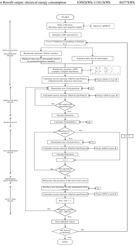
In the M&V baseline energy model phase, the baseline energy model was developed using CV resampling techniques since limited data were available for this study. The CV resampling techniques were introduced to improve the prediction accuracy of Option C. These techniques also overcome the problem of overfitting, to check the model robustness and generalisation abilities for a small data application in predicting energy consumption for Option C.ABC optimization was applied to develop the HANN baseline energy model. ABC was embedded with CV to train the network to optimise the synaptic weights and biases and predict the baseline energy consumption. A step-by-step flowchart of the HANN-CV model development is shown in Figure 2. Once all the setting has been determined, the CV resampling techniques were applied to split the data set into training, validation, and testing sets. Then, the ABC optimisation technique was executed and fitness for each set of data was evaluated by calling the ANN programme, where ANN was trained to maximise the fitness which was coefficient of correlation (R).
ABC is also a swarm-based optimisation technique, proposed by [26]. It is inspired by the foraging behaviour of bees to find the optimal solution. Generally, ABC optimisation is composed by four main phases, which are initialisation, employed bee, onlooker bee, and scout bee phases. In addition, the proposed HANN-CV technique was implemented using the following steps:
1. In the initialisation phase, the ABC control parameters were prescribed. There are three control parameters: the colony size, the food number and the maximum cycle number. The number of parameters to be optimised, D was based on the number of neurons in the hidden layer. In this work, the optimised parameters are the number of synaptic weights and biases.
2. ABC randomly generated initial population (foods) which are initial weights and biases using (1). The initial population was evaluated by calling the ANN programme, where ANN was trained to maximise the fitness which is the coefficient of correlation and calculate the fitness values as (2).
𝑋𝑖𝑗= 𝑋𝑚𝑖𝑛𝑗 + 𝑟𝑎𝑛𝑑(0,1)(𝑋𝑚𝑎𝑥 𝑗
− 𝑋𝑚𝑖𝑛𝑗 ) (1)
𝑓𝑖𝑡𝑖= { 1
1+𝑓𝑖, 𝑓𝑖≥ 0
1 + 𝑎𝑏𝑠(𝑓𝑖), 𝑓𝑖< 0
(2)
Where 𝑋𝑖𝑗 is the initial population or initial foods (current candidate solution), the parameters to be optimised, 𝑋𝑚𝑖𝑛𝑗 is the lower bound of the parameter, 𝑋𝑚𝑎𝑥
𝑗
fitness, and 𝑓𝑖 is the fitness of the solution. Then, the best fitness value and foods were recorded.
3. In the employed bee phase, the new candidate solutions or new foods were produced from its neighbouring solution, using (3).
𝑉𝑖,𝑗 = 𝑋𝑖,𝑗+ ∅𝑖,𝑗(𝑋𝑖,𝑗− 𝑋𝑗.𝑘) (3)
Where 𝑉𝑖,𝑗 is the new candidate solution, 𝑋𝑖,𝑗 is the current candidate solution, 𝑋𝑗.𝑘is the neighbouring candidate solution, and ∅𝑖,𝑗 is a random number between −1 and 1.
4. Then, the fitness was evaluated for each set of food by calling the ANN programme. Greedy selection was applied between the current candidate solution and the new candidate solution. If the fitness of the food source of the employed bee better than the current candidate solution, the solution is replaced with the new candidate and the trial counter is reset.
5. In the onlooker bee phase, the new candidate solutions were produced according to (3) depending on the probability, 𝑝𝑖 as in (4). The probability was selected using Roulette Wheel selection mechanism. Then, Greedy Selection was applied between the new candidate and the current candidate to select the better solution.
𝑝𝑖= 𝑓𝑖𝑡𝑖
∑𝑆𝑁𝑘=1𝑓𝑖𝑡𝑛 (4)
6. The position of the best food source was memorized and recorded. If the position cannot be improved or a predefined limit, then the food source is abandoned.
7. Therefore, in the scout bee phase, to discover the abandoned solution and replace it with the new solution, the scout bee randomly searched using (1). Then, the ANN was called and evaluated for a new solution. The best fitness value and food source were recorded.
8. The process continued until the maximum cycle number was reached. The iteration will stop executed when all the datasets have been trained and evaluated. In this case, the networks run for 5 times due to the 5-fold of CV dataset were created. Then, the average values of all performance functions were calculated and saved.
The R performance of HANN-CV and ANN-CV [25] in all baseline energy models were compared. The higher R indicates the strong correlation between the targeted and the predicted output, was selected as the best model and used for predicting the adjusted baseline model in the post-retrofit saving calculation phase as well as determining energy saving
2.2. Applying HANN model for determining energy savings in post-retrofit
In this phase, the post-retrofit data were used to determine the adjusted baseline to quantify savings. In principle, M&V quantifies energy savings by comparing energy consumption before and after the retrofitting process. The energy consumption after the retrofitting process is known as the post-retrofit energy consumption. The post-retrofit input data were loaded into the HANN-CV baseline energy model to predict the output. The predicted output is known as the adjusted baseline energy. Savings in terms of energy avoided were determined from the differences between the adjusted baseline energy and post-retrofit energy consumption as in (5).
𝐸𝑎= 𝐸𝑎𝑏− 𝐸𝑝𝑟 (5)
Where 𝐸𝑎 is the energy avoided, 𝐸𝑎𝑏 is the adjusted baseline energy, and 𝐸𝑝𝑟is the post-retrofit energy consumption.
2.3. Data collection
For Option C, the baseline and post-retrofit data were obtained on monthly basis from the Facility Management Office, Universiti Teknologi Mara (UiTM), Shah Alam, Selangor, Malaysia, except CDD. The CDD data were obtained from Malaysian Meteorological Department. The whole dataset of Faculty of Electrical Engineering, UiTM is presented as in Table 1 with the minimum, maximum, and mean values.
The data were divided into two types: 1) 23 monthly energy and independent variables baseline data in 2012 to 2014 and 2) 20 monthly post-retrofit data from 2014 to 2016. Three input variables were measured in developing the baseline energy model: working days, class days and cooling degree days. These parameters were assigned as ANN input and the targeted output for the baseline which was the monthly electricity consumption.
Table 1. Option C IPMVP – statistical data for baseline and post-retrofit
Parameter Range Mean
Baseline input: class days 0 – 21 14
Baseline input: cooling degree days 468 – 628 563
Baseline input: working days 21 3.143°C
Baseline output: electrical energy consumption 109642kWh-159226kWh 138507kWh
Post Retrofit input: class days 0 – 23 14
Post Retrofit input: cooling degree days 511 – 649 579
Post Retrofit input: working days 17 – 23 21
Post Retrofit output: electrical energy consumption 63002kWh-113613kWh 86377kWh
START
Initialize ABC parameters
Calculate nectar amount: ObjVal and Fitness (Optimized the objective function)
Determine new food position
Calculate nectar amount: ObjVal and Fitness
No
Calculate Probabilities Yes
Yes No
Determine new food position
Calculate nectar amount: ObjVal and Fitness Greedy Selection
Greedy Selection
All onlookers distributed?
Memorize the position of the best food source i=i+1
No
Yes
Produce new position for the abandoned food source.
Calculate nectar amount: ObjVal and Fitness
Stopping criteria Iter >MCN? No
Yes Iter =iter + 1 Randomly generate ANN synaptic weights and biases
Train ANN to max R
All employed Distributed?
INITIALIZATION & RESAMPLING
PHASE
Random no < prob(i)?
EMPLOYED BEE PHASE
PROBABALITY
ONLOOKER BEE PHASE
SCOUT BEE PHASE MEMORIZE BEST POSITION
Train ANN to max R
Train ANN to max R Train ANN to max R
Save optimal values Randomly generate indices number
Partition data into k-subsamples Partition data into k-subsamples based
on generated indices number
Cross Validation resampling technique k=1
END All dataset evaluated?
k=k+1 Data collection:
Baseline input and targeted output Option C IPMVP
Yes No
3. RESULTS AND DISCUSSION
This section explains the result of baseline energy model using CV resampling techniques which were incorporated with ANN and ABC. The HANN and ANN methods from the previous paper were compared at the end of this section. The performance between the targeted and predicted output were evaluated and compared to find the most accurate method. The model with the highest values of R was selected as the most accurate baseline energy model and used in the post retrofit phase to calculate the adjusted baseline energy model, hence to determine the energy saving.
3.1. Baseline energy model development results
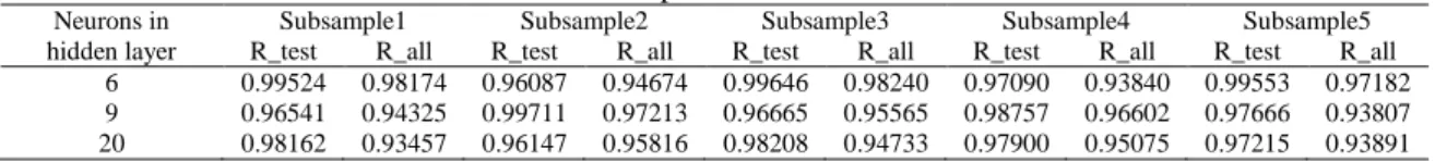
The network configurations with 6, 9, and 20 neurons in the hidden layer were applied to HANN-CV. In this study, ABC was implemented in ANN and evaluated together with the CV method to avoid trial and error method and increase the accuracy of the energy baseline model. For each selected neuron in the hidden layer, five iterations of training, validation, and testing sets were performed, and the performance of each fold was measured performance evaluation functions. The average Rtest and Rall values for each subsample is tabulated in Table 2. From Table 2, the average Rtest and Rall values for all subsamples were above 0.93, indicates a close match between the measured and predicted energy consumption during the testing and overall training processes.
In order to clearly show the overall performance of ANN-CV and HANN-CV with the combination of 6, 9, and 20 neurons in the hidden layer, these models were compared to each other as shown in Table 3. In comparison to ANN-CV method, the average R values of HANN-CV obtained better results in terms of accuracy and robustness. This research finds out that the resampling technique with HANN, was able to produce better result and predict a more accurate energy consumption than the methods with ANN-CV. The values for all average coefficient of correlation for HANN method were greater than 0.86. These results indicate the HANN method with limited data available avoid network overfitting and produce a very high prediction accuracy model. On average, HANN-CV model with 6 neurons in the hidden layer have higher average accuracy compared to the other two models. Even though the R_valid values were lower than the other values, it was still acceptable and met the IPMVP requirement. The capability of ANN to learn and predict is supported by the degree of acceptability of the training, validation, and testing sets performance.
Table 2. The effect of number of neurons in hidden layer on average coefficient of correlation of subsamples R_test and R_all for option C IPMVP – HANN-CV.
Neurons in hidden layer
Subsample1 Subsample2 Subsample3 Subsample4 Subsample5
R_test R_all R_test R_all R_test R_all R_test R_all R_test R_all
6 0.99524 0.98174 0.96087 0.94674 0.99646 0.98240 0.97090 0.93840 0.99553 0.97182
9 0.96541 0.94325 0.99711 0.97213 0.96665 0.95565 0.98757 0.96602 0.97666 0.93807
20 0.98162 0.93457 0.96147 0.95816 0.98208 0.94733 0.97900 0.95075 0.97215 0.93891
Table 3. The effect of number of neurons in hidden layer on R for option C IPMVP – Comparison between ANN-CV and HANN-CV
Neurons in hidden layer
HANN-CV ANN_CV
R_train R_valid R_test R_all R_train R_valid R_test R_all
6 0.979313 0.888665 0.983800 0.964222 0.899510 0.759100 0.858070 0.872480
9 0.964473 0.866787 0.978680 0.955025 0.891283 0.728845 0.871952 0.873129
20 0.952449 0.888990 0.975262 0.945944 0.907072 0.848054 0.811169 0.862649
Even though the HANN-CV model with 6 neurons in hidden layer has much better prediction results than the model with 9 and 20 neurons in hidden layer based on the average value, the model with 20 neurons was chosen as the best model based on the highest values of all coefficient of correlation results, R_train, R_valid, R_test and R_all. This selected model achieved the R_all of 0.990890 and R_train of 0.999016, R_valid of 0.978461, and R_test of 0.999710. The values for all R were greater than 0.98 which considered acceptable and in compliance with the IPMVP protocol.
3.2. Applying hybrid ANN model for determining energy savings in Post Retrofit
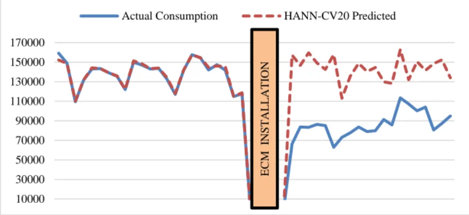
In order to quantify energy saving, the adjusted baseline model need to be developed. Therefore, the HANN-CV model with 20 neurons in the hidden layer was applied to the post-retrofit data for Option C to develop the adjusted baseline model. The M&V timeline for Option C is graphically shown in Figure 3. The figure illustrates the whole data for 23 months for the baseline period and 20 months for the post retrofit
period. The graph shows the actual energy consumption for the baseline and post-retrofit, the HANN-CV predicted values for the baseline and post-retrofit for the given timeline. The predicted values for post-retrofit period was also known as adjusted baseline. From the figure, a bigger gap was present between the adjusted baseline and actual consumption in the post-retrofit period. This gap represents the energy saving obtained, the difference between the adjusted baseline and energy consumption for the post-retrofit period.
Therefore, the energy savings obtained for 20 months was 1,149,491.56 kWh ± 0.48% at 95% of confidence level with 39.95% of energy savings. The relative precision was computed using a t value from the normal t-distribution table. The uncertainty presented in the savings complied with the requirements by the IPMVP which the standard error of the baseline value should be more than twice.
Figure 3. M&V Timeline for Option C-IPMVP.
4. CONCLUSION
The application of HANN-CV for modelling the baseline energy for small dataset was presented in this study to improve the learning accuracy of a small dataset problems in the prediction of energy consumption of Option C. The ABC optimisation was used and embedded in this method to find the optimum values of weights and biases to enhance the prediction of the baseline energy model.
The presented results in the previous section shows that the resampling techniques are capable to train the neural network even with limited data available. Apart from that, the results show that the baseline model with HANN performed better than ANN in terms of the predicting ability and accuracy. The predicted values obtained by HANN model corresponded closely to the measured values (targeted output) and quite satisfactory correlation where the average was more than 84% for training, testing, and validation sets. The most appropriate and accurate method for Option C is HANN-CV model with 20 neurons, where the percentage of all Rs were 97.85%, which can be considered very highly correlated.
This approach proves to be a very promising alternative to the Option C and this proposed method can improve learning performance significantly when working with small dataset.
REFERENCES
[1] J. Granderson, S. Touzani, C. Custodio, M. D. Sohn, D. Jump, and S. Fernandes, “Accuracy of automated measurement and verification (M&V) techniques for energy savings in commercial buildings,” Appl. Energy, vol. 173, pp. 296–308, 2016.
[2] G. L. Gouws, R, ME Storm, “Measurement & Verification of the Eskom Irrigation Pumping Standard Product Programme,” in Industrial and Commercial Use of Energy Conference (ICUE), 2013 Proceedings of the 10th, 2013.
[3] Efficiency Valuation Organization, “International Performance Measurement and Verification Protocol (IPMVP),” 2012.
[4] D. De Canha, “Measurement & Verification of Coal Fired Power Station Maintenance Projects,” in Power Engineering Conference (AUPEC), 2015 Australasian Universities, 2015, pp. 1–5.
[5] B. G. Menita et al., “Measurement and Verification in Energy Efficiency Projects involving Solar Water Heating Systems in Homes of Low-Income Families – Case Studies,” in 2015 CHILEAN Conference on Electrical, Electronics Engineering, Information and Communication Technologies (CHILECON), 2015, pp. 585–590. [6] J. Meng, L. Jiang, F. Liu, J. Zheng, and Q. Li, “A measurement and verification method for energy savings of
power line transformation project,” China Int. Conf. Electr. Distrib. CICED, vol. 2014-Decem, no. Ciced, pp. 738– 744, 2014.
10000 30000 50000 70000 90000 110000 130000 150000 170000
Actual Consumption HANN-CV20 Predicted
EC
M
IN
S
T
A
L
L
A
TI
O
[7] A. Martinez and J. Choi, “Analysis of energy impacts of facade-inclusive retrofit strategies , compared to system-only retrofits using regression models,” Energy Build., vol. 158, pp. 261–267, 2018.
[8] M. Zeifman, A. Prediction, and E. Propensity, “Measurement and Verification of Energy Saving in Smart Building Technologies,” in Signal Processing Applications in Smart Buildings, 2015, pp. 343–347.
[9] R. F. Mustapa, “Baseline Energy Modelling in an Educational Building Campus for Measurement and Verification,” in 2017 International Conference on Electrical, Electronics and System Engineering (ICEESE), 2017, pp. 67–72.
[10] S. M. Aris, N. Y. Dahlan, M. N. M. Nawi, T. A. Nizam, and M. Z. Tahir, “Quantifying Energy Savings for Retrofit Centralized HVAC Systems at Selangor State Secretary Complex,” J. Teknol., vol. 77, no. 5, pp. 93–100, 2015. [11] X. Ye and X. Xia, “Optimal metering plan for measurement and verification on a lighting case study,” Energy, vol.
95, pp. 580–592, 2016.
[12] M. Coroiu and M. Chindris, “Energy efficiency indicators and methodology for evaluation of energy performance and retained savings,” in 2014 49th International Universities Power Engineering Conference (UPEC), 2014, pp. 1–6.
[13] C. Coetzee, C. A. Van Der Merwe, and P. L. J. Grobler, “Basic Measurement and Verification Approach for Roll-Out Programmes,” in Industrial and Commercial Use of Energy Conference (ICUE), 2012 Proceedings of the 9th, 2012.
[14] X. Xia, X. Ye, and J. Zhang, “Optimal Metering Plan of Measurement and Verification for Energy Efficiency Lighting Projects,” in 2012 Southern African Energy Efficiency Convention (SAEEC), 2012, pp. 1–8.
[15] O. Akinsooto, D. De Canha, and J. H. C. Pretorius, “Energy Savings Reporting and Uncertainty in Measurement & Verification,” in Australasian Universities Power Engineering Conference, AUPEC 2014, Curtin University, Perth, Australia, 2014, no. October, pp. 1–5.
[16] F. Rodríguez, A. Fleetwood, A. Galarza, and L. Fontán, “Predicting solar energy generation through artificial neural networks using weather forecasts for microgrid control,” Renew. Energy, vol. 126, pp. 855–864, 2018. [17] I. I. Argatov and Y. S. Chai, “Tribology International An artificial neural network supported regression model for
wear rate,” Tribiology Int., vol. 138, no. January, pp. 211–214, 2019.
[18] F. N. Osuolale and J. Zhang, “Energy efficiency optimisation for distillation column using artificial neural network models,” Energy, vol. 106, pp. 562–578, 2016.
[19] A. H. A. Al-waeli, K. Sopian, J. H. Yousif, H. A. Kazem, J. Boland, and M. T. Chaichan, “Artificial neural network modeling and analysis of photovoltaic / thermal system based on the experimental study,” Energy Convers. Manag., vol. 186, no. November 2018, pp. 368–379, 2019.
[20] H. Suyono, R. N. Hasanah, P. Mudjirahardjo, M. F. E. Purnomo, and S. Uliyani, “Enhancement of the power system distribution reliability using ant colony optimization and simulated annealing methods,” Indones. J. Electr. Eng. Comput. Sci., vol. 17, no. 2, pp. 877–885, 2020.
[21] M. N. Kamarudin, T. Juhana, and T. Hashim, “Coordinated and optimal voltage control for voltage regulation using firefly algorithm,” Indones. J. Electr. Eng. Comput. Sci., vol. 16, no. 2, pp. 568–576, 2019.
[22] Y.-L. H. Hong-Fei Gong, Zhong-Sheng Chen, Qun-Ciong Zhu, “A Monte Carlo and PSO based virtual sample generation method for enhancing the energy prediction and energy optimization on small data problem: An empirical study of petrochemical industries,” Appl. Energy, vol. 197, pp. 405–415, 2017.
[23] D. K. Barrow and S. F. Crone, “Cross-validation aggregation for combining autoregressive neural network forecasts,” Int. J. Forecast., vol. 32, no. 4, pp. 1120–1137, 2016.
[24] M. Saltan and S. Terzi, “Modeling deflection basin using artificial neural networks with cross-validation technique in backcalculating flexible pavement layer moduli,” Adv. Eng. Softw., vol. 39, no. 7, pp. 588–592, 2008.
[25] W. N. W. Md Adnan, N. Y. Dahlan, and I. Musirin, “Modeling baseline energy using artificial neural network: A small dataset approach,” Indones. J. Electr. Eng. Comput. Sci., vol. 12, no. 2, pp. 662–669, 2018.