Optimal Size and Location of Distributed Generations for Minimizing Power Losses in a Primary Distribution Network

Vol. 16, No. 2, pp. 137{144 c

Sharif University of Technology, December 2009

Optimal Size and Location of Distributed

Generations for Minimizing Power Losses

in a Primary Distribution Network

R.M. Kamel

_{and B. Kermanshahi}

Abstract. Power system deregulation and shortage of transmission capacities have led to an increase interest in Distributed Generations (DGs) sources. The optimal location of DGs in power systems is very important for obtaining their maximum potential benets. This paper presents an algorithm to obtain the optimum size and optimum location of the DGs at any bus in the distribution network. The proposed algorithm is based on minimizing power losses in the primary distribution network. The developed algorithm can also be used to determine the optimum size and optimum location of the DGs embedded in the distribution network, including power cost and the available rating of DGs if the DGs exist in a competitive market. An algorithm is applied to three test distribution systems with dierent sizes (6 buses, 18 buses and 30 buses). Results indicated that, if the DGs are located at their optimal locations and have optimal sizes, the total losses in the distribution network will be reduced by nearly 85%. The results can be used as a look-up table, which can help design engineers when inserting DGs into the distribution networks.

Keywords: Distributed generation; Optimal location; Optimal size; Loss minimization.

INTRODUCTION

Distributed generation is an electric power source connected directly to the distribution network or cus-tomer side of the meter [1]. It may be explained in simple terms that is small-scale electricity generation takes dierent forms in dierent markets and countries and is dened dierently by dierent agencies. The International Energy Agency (IEA) denes distributed generation as a generating plant, serving a customer on-site or providing support to a distribution network connected to the grid at distribution-level voltages [1]. CIGRE denes DG as the generation that has the following characteristics [2]: It is not centrally planned; it is not centrally dispatched at present; it is usually connected to the distribution network; it is smaller than 50-100 MW. Other organizations like the Electric Power Research Institute (EPRI) denes a distributed generation as the generation from a few kilowatts up

1. Department of Electronics and Information Engineering, Tokyo University of Agriculture and Technology, Tokyo, P.O. Box 184-0012, Japan.

*. Corresponding author. E-mail: [email protected] Received 18 July 2008; received in revised form 31 October 2008; accepted 29 December 2008

to 50 MW [3]. In general, DG means small scale generation.

There are a number of DG technologies available in the market today and a few are still at the research and development stage. Some currently available technologies are: reciprocating engines, micro turbines, combustion gas turbines, fuel cells, photovoltaic sys-tems and wind turbines. Each of these technologies has its own benets and characteristics. Among all DGs, diesel or gas reciprocating engines and gas turbines make up most of the capacity installed so far. Simultaneously, new DG technology, like micro turbines, is being introduced and older technology, like reciprocating engines, is being improved [1]. Fuel cells are the technology of the future, however, there are some prototype demonstration projects. The cost of photovoltaic systems is expected to fall continuously over the next decade. These statements obviously indicate that the future of power generation is DG.

The share of DGs in power systems has been fast increasing in the last few years. According to the CIGRE report [2], the contribution of DG in Denmark and the Netherlands has reached 37% and 40%, respectively, as a result of the liberalization of the power market in Europe. The EPRI study forecasts

that 25% of the new generation will be distributed by 2010 and a similar study by the Natural Gas Foundation believes that the share of DG in the new generation will be 30% by the year 2010 [4]. The numbers may vary as dierent agencies dene DG in dierent ways. However, with the Kyoto protocol put in place, where there will be a favorable market for DGs that are coming from \Green Technologies", the share of DG will increase and there is no sign that it will decrease in the near future. Moreover, the policy initiatives to promote DG throughout the world also indicate that the number will grow rapidly. As the penetration of DG in distribution systems increases, it is in the best interest of all players involved to allocate DG in such an optimal way that it will reduce system losses, hence improve the voltage prole.

Studies have indicated that inappropriate selec-tion of the locaselec-tion and size of DG may lead to greater system losses than losses without DG [5,6]. Utilities already facing the problem of high power loss and poor voltage proles cannot tolerate any increase in losses. By optimum allocation, utilities take advantage of a reduction in system losses, improved voltage regulation and an improvement in the reliability of supply [5-7]. It will also relieve the capacity of transmission and distribution systems and hence defer new investments which have a long lead-time.

DG could be considered as one of the most viable options to ease some of the problems (e.g. high loss, low reliability, poor power quality and congestion in transmission systems) faced by power systems, apart from meeting the energy demand of ever growing loads. In addition, the modular and small size of the DG will facilitate the planner to install it in a shorter time frame compared to the conventional solution. It would be more benecial to install in a more decentralized environment where there is a larger uncertainty in demand and supply. However, given the choices, they need to be placed in appropriate locations with suitable sizes. Therefore, analysis tools are needed to be developed to examine locations and the sizing of such DG installations.

The optimum DG allocation can be treated as optimum active power compensations, like capacitor allocation for reactive power compensation. This paper modied the economic dispatch method to determine the optimum size and location of DG in the distribution network. The power cost and rating limits of DG can be taken into consideration. The proposed algorithm is suitable for the allocation of single or multiple DGs in a given distribution network.

The rest of the paper is organized as follows: First a brief review of the previous research on determining DGs optimum size and location is presented. Then a complete description of the proposed algorithm and a ow chart of the developed programs are oered. After

that, three dierent size distribution systems used in the paper are described, and results and discussions are given. Finally, conclusions are presented.

REVIEW OF THE PREVIOUS METHODS USED FOR OPTIUMUM LOCATION OF DG IN THE DISTRIBUTION NETWORK DG allocation studies are relatively new, unlike ca-pacitor allocation. In [8,9], a power ow algorithm is presented to nd the optimum DG size at each load bus, assuming every load bus can have a DG source. The Genetic Algorithm (GA) based method to determine size and location is used in [10-12]. GA's are suitable for multi-objective problems like DG allo-cation, and can give near optimal results, but they are computationally demanding and slow in convergence. Grin [6] uses a loss sensitivity factor method and Naresh [13] proposes an analytical method to determine the optimal size and location of DG in distribution networks; these two methods are briey described in the following sections respectively.

Loss Sensitivity Factor Method

The loss sensitivity factor method is based on the principle of linearization of the original nonlinear equa-tion (loss equaequa-tion) around the initial operating point, which helps to reduce the amount of solution space. The loss sensitivity factor method has been widely used to solve the capacitor allocation problem. Its application in DG allocation is new in the eld and has been reported in [6].

Loss Sensitivity

The real power loss in a system is given by Equation 1. This is popularly referred to as the \exact loss" for-mula [14]:

PL= N

X

i=1 N

X

j=1

[ij(PiPj+QiQj)+ij(QiPj PiQj)];

(1) where:

ij=_Vrij

iVj cos(i j); ij=

rij

ViVjsin(i j);

and rij+ jxij = Zij are the ijth element of [Zbus].

The sensitivity factor of real power loss with respect to a real power injection from DG is given by:

i= @P_@PL i = 2

N

X

i=1

(ijPj ijQj): (2)

Sensitivity factors are evaluated at each bus, rstly, using the value obtained from the base case power ow.

The buses are ranked in descending order of the values of their sensitivity factors to form a priority list. The top-ranked buses in the priority list are the rst to be studied as alternative locations.

Priority List

The sensitivity factor will reduce the solution space to a few buses, which constitute top ranking in the priority list. The eect of the number of buses taken in priority will aect the optimum solution obtained for some systems. For each bus in the priority list, the DG is placed and the size of the DG is varied from minimum (0 MW) to a higher value until the minimum system losses are found with the DG size. The process is computationally demanding as a large amount of load ow solution is needed, and this may not determine exactly the size and location of the DG, as varying the size of the DG will be in steps.

Analytical Method for Optimal Size and Location of DG

In [13], a new methodology is proposed to nd the optimum size and location of DG in the distribution system. This methodology requires load ow to be carried out only twice, once for the base case and once at the end, with DG included, to obtain the nal solution.

Sizing at Various Locations

The total power loss against injected power is a parabolic function and, at minimum losses, the rate of change of loss with respect to the injected power becomes zero [13]:

@PL

@Pi = 2 N

X

i=1

(ijPj ijQj) = 0: (3)

It follows that: iiPi ijQi+

N

X

j=1;j6=i

(ijPj ijQj) = 0;

Pi=1 ii

2 4iiQi+

N

X

j=1;j6=i

(ijPj ijQj)

3

5 ; (4)

where Pi is the real power injection at node i which is

the dierence between real power generation and real power demand at that node:

Pi= (PDGi PDi); (5)

where PDGi is the real power injection from DG placed

at node i, and PDi is the load demand at node i. By

combining Equations 4 and 5, one can get Equation 6: PDGi=PDi+1

ii

2 4iiQi

N

X

j=1;j6=i

(ijPj ijQj)

3 5 :

(6) Equation 6 gives the optimum size of DG for each bus i, for the loss to be minimum. Any size of DG other than PDGiplaced at bus i, will lead to higher loss. This

loss, however, is a function of loss coecient and . When DG is installed in the system, the values of the loss coecients will change, as it depends on the state variable voltage and angle; this is the disadvantage of this method. After DG is installed, the values of the voltages and angles at all buses have signicant changes and this may lead to a high error in the optimal size obtained by Equation 6.

PROPOSED ALGORITHM

In our analysis, we consider the problem in general and determine the optimal size and location of the DG, taking power losses and cost into consideration in addition to the available power rating limits of DG. Mathematical Analysis of the Proposed

Algorithm

The fuel cost of the generator at bus i can be repre-sented as a quadratic function of real power generation (Pi) [15]:

ci = i+ iPi+ iPi2; (7)

where i, iand iare the cost coecients of generator

i ( $/h, $/MWh, $/MWh2_).

If the power system contains N generators, the total cost is given by the following equation:

ct= N

X

i=1

Ci = N

X

i=1

i+ iPi+ iPi2: (8)

The system losses are included in the optimization process. One common practice for including the eect of losses is to express total system losses as a quadratic function of the generator power outputs. The simplest quadratic form is:

PL= N

X

i=1 N

X

j=1

PiBijPj: (9)

A more general formula, containing a linear and a constant term, and referred to as Kron's formula is [15]:

PL= N

X

i=1 N

X

j=1

PiBijPj+ N

X

i=1

The coecients Bij are called loss coecient or

B-coecients.

The power output of any generator should not ex-ceed its rating, nor should it be below that necessary for stable operation. Thus, the generations are restricted to lie within given minimum and maximum limits.

The optimization process aims to minimize the overall generating cost, Ct, given by Equation 8,

subject to the constraint that generation should be equal to total demands (PD) plus losses (PL):

N

X

i=1

Pi= PD+ PL: (11)

Also, satisfying the inequality constraints of generators, the power limit is expressed as follows:

Pi(min) Pi Pi(max); i = 1; 2; ; N; (12)

where Pi(min) and Pi(max)are the minimum and

maxi-mum generating limits, respectively, for generator i. Using the Lagrange multiplier and adding addi-tional terms to include the inequality constraints, we obtain [15]:

L = Ct+ PD+ PL N

X

i=1

Pi

!

+XN

i=1

i(max)(Pi Pi(max))

+XN

i=1

i(min)(Pi Pi(min)); (13)

where:

: is the incremental power cost,

i(min): is the factor which takes the minimum

generation power limit of generator i, i(max): is the factor to take the maximum

generation power limit of generator i. The minimum of this unconstrained function is found at the point where the partials of the function to its variable are zero:

@L

@Pi = 0; (14)

@L

@ = 0; (15)

@L

@i(max) = Pi Pi(max)= 0; (16)

@L

@i(min) = Pi Pi(min) = 0: (17)

Equations 16 and 17 imply that Pi should not be

allowed to go beyond its limits, and when Pi is within

its limits, then i(min) = i(max) = 0. The rst

condition given by Equation 14 results in: @Ct

@Pi +

0 + @P_@PL

i 1

= 0: (18)

Since:

Ct= C1+ C2+ + CN:

Then: @Ct

@Pi =

dCi

dPi: (19)

And therefore the condition for optimum dispatch is: dCi

dPi +

@PL

@Pi = ; i = 1; 2; ; N: (20)

The second condition given by Equation 15 results in Equation 21:

N

X

i=1

Pi = PD+ PL: (21)

Equation 20 can be rearranged as: 1

1 @PL

@Pi

! dCi

dPi = ; i = 1; 2; ; N: (22)

The incremental power losses are obtained from the loss formula given by Equation 10 and results in Equation 23:

@PL

@Pi = 2 N

X

j=1

BijPj+ B0i: (23)

Substituting Equation 23 in Equation 20 results in Equation 24:

i

+ Bii

Pi+ N

X

j=1 j6=i

BijPi=1₂

1 B0i Bi

: (24) Extending Equation 24 to all generators results in the following linear equations in matrix form:

2 6 6 4

1

+ B11 B12 B1N

B21 2 + B22 B2N

BN1 BN2 N + BNN

3 7 7 5 2 6 6 4 P1 P2 PN 3 7 7 5

=1₂ 2 6 6 4

1 B01 B1

1 B02 B2

1 B0N BN

3 7 7

or in short form:

EP = D: (26)

To nd the optimal for an estimated value of (1)

(Initial value of the incremental power cost), the simultaneous linear equation given by Equation 25 is solved. Then, the iterative process is continued using the gradient method [15]. To do this, from Equation 24, Pi at the kth iteration is expressed as:

P_i(k)=

(k)_{(1 B}

0i) i 2(k) N

P

j=1 j6=i

BijPj(k)

2(i+ (k)Bii) : (27)

Substituting for Pi from Equation 27 in Equation 11

results in Equation 28:

N

X

i=1

(k)_{(1 B}

0i) i 2(k)P j6=iBijP

(k) j

2(i+ (k)Bii) =PD+P (k) L ;

(28) or:

f()(k)_{= P}

D+ P_L(k): (29)

Expanding the left-hand side of Equation 29 in the Tay-lor series about an operating point, (k)_{, and neglecting}

the higher-order terms results in Equation 30: f()(k)₊

df()

d _(k)

(k)_{= P}

D+ PL(k); (30)

or:

(k)₌ P(k) df()

d

_(k) = PP_dP(k)_i

d

(k); (31)

where:

N

X

i=1

@Pi

@ (k)

=

N

X

i=1

i(1 B0i)+Biii 2iP j6=iBijP

(k) j

2(i+ (k)Bii)2 ₍₃₂₎;

and, therefore:

(k+1)₌ (k)₊ (k)_{; (33)}

where: P(k)_{= P}

D+ PL(k) N

X

i=1

P_i(k): (34)

The process is continued until P(k) _{is less than a}

specied accuracy.

A program named \Bloss" is developed for com-putation of the B-coecient. This program requires

the power ow solution. Another program called the \dispatch" of the generation is developed and this pro-gram produces a variable named \dpslack". This is the dierence (absolute value) between the scheduled slack generation determined from the coordination equation, and the slack generation obtained from the power ow solution. A power ow solution obtained with the new scheduling of generation results in new loss coecients, which can be used to solve the coordination equation again. This process can be continued until \dpslack" is within a specied tolerance ("). This can be explained in the ow chart in Figure 1. The result of this method is more accurate than the two methods described previously, because during each load ow calculation, the losses coecients are updated for the new generation dispatch. Also, another advantage of the proposed algorithm is that the DG power limits are taken into consideration.

TEST SYSTEMS AND ANALYTICAL TOOLS

The proposed algorithm is tested on three dierent test systems with dierent sizes to show that it can be implemented in distribution systems of various con-gurations and sizes. The rst system (25-KV IEEE-6-bus systems) is shown in Figure 2 [16], which can be considered as a subtransmission/distribution system, which was applied to verify the algorithm described previously. The parameters of this system are given in [16]. The second test system is a part of the IEEE 30-bus system, as shown in Figure 3, which can be considered as a meshed transmission/subtransmission

Figure 1. Flow chart of the used and developed programs.

system. The system has 30 buses (mainly 132 and 33 KV buses) and 41 lines. Only 18 buses of this system is taken into consideration, so that this system is considered as an 18-bus system. The system bus data and line parameters are given in [15,16]. The third test system is a 30-bus distribution system, as depicted in Figure 4. The parameters of the system are found in [17].

A computer program has been written in MAT-LAB 7.2 to calculate the optimum sizes of the DG at

Figure 2. One-line diagram of 6-bus system.

Figure 3. IEEE 30-bus test system.

Figure 4. One line diagram of 30-bus system.

various buses and power losses, with the DG at dierent locations to identify the best location. A Newton-Raphson algorithm based load ow program is used to solve the load ow problem.

SIMULATION RESULTS Sizes Allocation

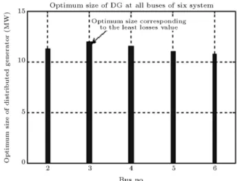
In our calculation, the optimum size and optimum location are determined based on minimizing power losses only. If the DG exists in a competitive market, the optimum size and location can be determined based on cost, loss minimizing and available ratings. Based on the algorithm described before, the optimum sizes of DG are calculated at various nodes for the three test systems. Figures 5, 6 and 7 show the optimum sizes of DG at various nodes for 6-, 18- and 30-bus distribution systems, respectively.

As far as one location is concerned, in a

distribu-Figure 5. Optimal size of DG for 6-bus system.

Figure 7. Optimal size of DG for 30-bus system.

tion test system, the corresponding gure would give the value of the DG size to have a \possible minimum" total loss.

Any regulatory body can use this as a look-up table for restricting the sizes of DG for minimizing total power losses in the system.

In the 6-bus distribution test system, the opti-mum sizes ranging from 10.72 MW to 11.98 MW are shown in Figure 5. For the 18-bus test system, the optimum size of DG is varied between 30 MW to 65 MW. The range of DG size for the 30-bus test system at various locations varied from 0.244 MW to 15.888 MW, however, it is important to identify the location where total power loss is at a minimum. This can be identied with the help of power losses calculated in each case.

Optimal Location Selection

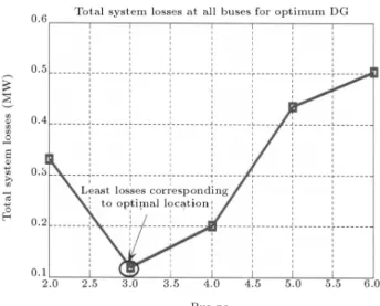
Figures 8, 9 and 10 show total power losses for 6-bus, 18-bus and 30-bus test systems, respectively, with optimum DG sizes obtained at various nodes of the respective systems. For each system, the best location can be determined directly from the loss gures (the bus corresponds to minimum losses).

For the 6-bus system, the best (optimum) location of the DG is bus 3 where total power losses are reduced to 0.1195 MW as depicted in Figure 8. The second best location is bus 4 where total power losses are 0.20106 MW. Each value of the losses is shown in Figure 8 and its corresponding optimum size is shown in Figure 5. For example, if the proposed DG is inserted at bus 2, the size of the DG and total system losses will be 11.2897 and 0.331595 MW, respectively, while if the proposed DG is inserted at bus 3, the size of the DG and total system losses will be 11.9663 and 0.1195 MW, respectively, and so on for other buses from 4 to 6. In all cases, only one DG inserted at a certain bus

Figure 8. Total power losses for 6-bus system.

Figure 9. Total power losses for 18-bus system.

Figure 10. Total power losses for 30-bus distribution system.

and at optimum size is calculated for active power loss minimization. After calculating the optimum size of the DG inserted at each bus individual, we look to the total results gure (like a map) and the least losses bus in the map (bus 3 in Figure 8), represents the optimum location of the proposed DG; its size can be obtained from Figure 5. The same is correct for the other two studied systems. In the 18-bus system, the optimum bus is bus 10 where total system losses are equal to 2.96 MW as shown in Figure 9. The corresponding optimum size of DG is 58.1905 MW, as shown in Figure 6. The second optimum location is bus 11 which corresponds to 3 MW power losses and a 57.5207 MW optimum size, as shown in Figures 9 and 6, respectively. In the 30-bus distribution test system, the best location is bus 12 with a total power loss of 0.312551 MW and 4.5342 MW optimum sizes as shown in Figures 10 and 7, respectively. The second best location is bus 11 with slightly higher total power losses as shown in Figure 10; its corresponding size is shown in Figure 7.

CONCLUSIONS

The size and location of DGs are crucial factors in the application of DG for loss minimization. This paper proposes an algorithm and develops two programs to calculate the optimum size of DG at various buses of the distribution system for minimizing power losses in the primary distribution network. The benet of the proposed algorithm for size calculation is that a look-up table can be created and used to restrict the size of the DG at dierent buses of the distribution system. The proposed algorithm is more accurate than previous methods and can identify the best location for single or multiple DG placements in order to minimize total power losses. The proposed method can be used to determine the optimum size and location of DG, taking into consideration the power cost and available power rating of DGs. The proposed method is applied to three test distribution systems. Results proved that the optimal size and location of a DG can save a huge amount of power. For the rst test system, power losses are reduced from 0.5 MW to 0.11 MW. In the second test system, losses are reduced from 13.5 MW to 2.96 MW, while in the third test system, losses are reduced from 2.5 MW to 0.31 MW. In practice, the choice of the best site may not be always possible due to many constraints, however, the analysis here showed that the losses arising from dierent placement varies greatly and hence this factor must be taken into consideration when determining an appropriate location.

REFERENCES

1. Distributed Generation in Liberalized Electricity Market, IEA Publication (2002), available at:

http://www.iea.org/dbtw-wpd/text-base/ nppdf/free /2002 /distributed2002.pdf

2. CIGRE, \Impact of increasing contribution of dis-persed generation on the power system", Working Group 37.23 (1999).

3. Thomas, A. et al. \Distributed generation: A def-inition", Electric Power Syst. Res., 57, pp. 195-204 (2001).

4. CIGRE, \CIGRE technical brochure on modeling new forms of generation and storage", (Nov. 2000), avail-able at: http://microgrids.power.ece.ntua.gr/doc 5. Mithulanan, N. et al. \Distributed generator

place-ment in power distributed generator placeplace-ment in power distribution system using genetic algorithm to reduce losses", TIJSAT, 9(3), pp. 55-62 (2004). 6. Grin, T. et al. \Placement of dispersed generation

systems for reduced losses", 33rd International Con-ference on Sciences, Hawaii (2000).

7. Borges, C. and Falcao, D. \Impact of distributed generation allocation and sizing on reliability, losses and voltage prole", in Proceedings of IEEE Bologna, Power Technology Conference (2003).

8. Row, N. and Wan, Y. \Optimum location of resources in distributed planning", IEEE Trans PWRS, 9(4), pp. 2014-2020 (1994).

9. Kim, J.O. et al. \Dispersed generation planning using improved Hereford ranch algorithm", Electric Power Syst. Res., 47(1), pp. 47-55 (1998).

10. Kim, K. et al. \Dispersed generator placement using fuzzy-GA in distribution systems", in Proceeding of IEEE Power Engineering Society Summer Meeting, Chicago, pp. 1148-1153 (July 2002).

11. Silvestri, A. et al. \Distributed generation planning using genetic algorithms", Proceedings of International Conference on Electric Power Engineering, Power Tech., Budapest, p. 99 (1999).

12. Carpinelli, G. et al. \Distributed generation sitting and sizing under uncertainty", Proceedings IEEE Porto Power Technology (2001).

13. Naresh, A. \An analytical approach for DG allocation in primary distribution network", Electric Power and Energy Systems, pp. 669-678 (2006).

14. Elgerd, I.o., Electric Energy System Theory: An Intro-duction, McGraw-Hill (1971).

15. Saadat, H., Power System Analysis, McGraw-Hill (1999).

16. Caisheng, W. and Hashem, M. \Analytical approach for optimum placement of distributed generation sources in power systems", IEEE Trans. Power Syst., l19(4), pp. 2068-2075 (2004).

17. Goran, S. and Danny, P. \Simulation tool for closed loop price signal based energy market operation within microgrids", Microgrids project deliverable of task DG1 (Oct. 2003), available at http://microgrids. power. ece.ntua.gr/