Assessing Behavior in Context
Do Physicians Always Flee from
HMOs? New Results Using Dynamic
Panel Estimation Methods
Timothy T. Brown, Janet M. Coffman, Brian C. Quinn, Richard
M. Scheffler, and Douglas D. Schwalm
Objective. To assess the impact of changes in relative health maintenance organiza-tion (HMO) penetraorganiza-tion on changes in the physician-to-populaorganiza-tion ratio in California counties when changes in the economic conditions in California counties relative to the U.S. average are taken into account.
Data Sources. Data on physicians who practiced in California at any time from 1988 to 1998 were obtained from the AMA Masterfile. The analysis was restricted to active, patient care physicians, excluding medical residents. Data on other covariates in the model were obtained from the Bureau of Economic Analysis, InterStudy, the Area Resource File, and the California state government. Data were merged using county FIPS codes.
Study Design. Changes in the physician-to-population ratio in California counties include the effects of both intrastate migration and interstate migration. A reduced-form model was estimated using the Arellano–Bond dynamic panel estimator. Economic conditions in California relative to the U.S. were measured as the ratio of county-level real per capita income to national-level real per capita income. Relative HMO pen-etration in California was measured as the ratio of county-level HMO penpen-etration to HMO penetration in the U.S. relative HMO penetration was instrumented using five identifying variables to address potential endogeneity. Omitted-variable bias was con-trolled for by first differencing the model. The model also incorporated eight other covariates that may be associated with the demand for physicians: the percentage of the population enrolled in Medicaid, beds in short-term hospitals per 100,000 population, the percentage of the population that is black, the percentage of the population that is Hispanic, the percentage of the population that is Asian, the percentage of the pop-ulation that is below age 18, the percentage of the poppop-ulation that is aged 65 and older, and the percentage of the population that are new legal immigrants in a given year. All of the above variables were lagged one period. The lagged physician-to-population ratio was also included to control for the supply of physicians. Separate equations were estimated for primary care physicians and specialist physicians.
Principal Findings. Changes in lagged relative HMO penetration are negatively as-sociated with changes in specialist physicians per 100,000 population. However, this effect of HMO penetration is attenuated and at times reversed in areas where the
magnitude of the difference in relative economic conditions is sufficiently large. We did not find any statistically significant effects for primary care physicians.
Conclusions. Consistent with prior studies, we find that changes in physician supply are associated with changes in relative HMO penetration. Relative economic conditions are an important moderator of the effect of changes in relative HMO penetration on physician migration.
Key Words. Managed care organizations (e.g., HMOs/PPOs/IPAs), health work-force: distribution/incomes/training, econometrics
Physicians, like any other professional group, tend to locate in those areas in which they will maximize their incomes, other things equal. Previous studies have found that managed care reduces the earnings of physicians, particularly specialist physicians, by reducing the demand for specialist care both abso-lutely and relative to generalist care (Simon, Dranove, and White 1997, 1998; Hadley and Mitchell 1999, 2002).1Several studies that analyzed data from the late 1980s and early 1990s suggest that specialists have responded to these incentives. The studies found that the number of specialists grew more rapidly in areas in which a relatively low percentage of the population was enrolled in health maintenance organizations (HMOs) (Escarce et al. 2000; Polsky et al. 2000; Jiang and Begun 2002).
However, none of these studies focused on an important determinant of physician migration: relative economic conditions. We show that including a measure of these conditions gives important additional information about how physicians respond to changes in HMO penetration.
We present evidence consistent with previous research that shows, other things equal, that there is a negative relationship between changes in relative HMO penetration and changes in the specialist physician-to-population ratio. However, this relationship can be attenuated and even reversed in areas where relative economic conditions are sufficiently favorable. We did not find statistically significant effects for primary care physicians.
We start with a discussion of prior research, and then develop our con-ceptual framework, after which we present our empirical model, estimation method, and data sources. After showing the results of our analyses, we end with a discussion of the results, including their implications for health policy.
P
RIORS
TUDIESThree previous studies have examined the impact of changes in HMO pen-etration on changes in physician stock (Simon, Dranove, and White 1997; Escarce et al. 2000; Jiang and Begun 2002). Simon, Dranove, and White (1997) found that from 1985 to 1993, the numbers of anesthesiologists, pathologists, and radiologists grew less rapidly in states where physicians derived a rela-tively high percentage of revenue from managed care organizations. Jiang and Begun (2002) reported that the change in HMO penetration in metropolitan areas between 1985 and 1994 was positively associated with the change in the percentage of primary care physicians and negatively associated with the change in the percentage of surgical specialists. Escarce et al. (2000) found that metropolitan areas that experienced high rates of growth in HMO penetration from 1986 to 1996 experienced larger increases in the percentage of physi-cians who were generalists and smaller increases in the total number of phy-sicians and in the number of medical/surgical specialists. Escarce and colleagues’ findings are especially persuasive because they use instrumental variables to adjust for the potential endogeneity of HMO penetration and changes in the number of physicians.
Although previous studies of the impact of growth in HMO penetration on physician stock are highly informative, they have important methodolog-ical limitations. Prior studies used two periods of data separated in time by 8– 10 years in order to detect long-run trends in physician stock. This approach will accurately detect long-run movements of physicians, but cannot detect changes in the behavior of physicians that may occur in the shorter run be-tween the endpoints used. The detection of shorter-run changes in physician stock requires data from multiple time periods and alternative methodologies, both of which we employ in this study.
C
ONCEPTUALF
RAMEWORKcosts by tightly controlling the utilization of specialists while simultaneously providing generous coverage for primary care and preventive services. Tech-niques for controlling the use of specialists include prior authorization, refer-rals, utilization management, and practice guidelines. This strategy reduces demand for specialists and increases demand for primary care physicians among HMO enrollees. In markets with high rates of relative HMO pene-tration, these changes in demand are expected to foster a decrease in special-ists’ incomes and either an increase or no change in primary care physicians’ incomes. On the margin, specialists are expected to respond to a decrease in income by retiring, switching from patient care to nonpatient care activities, or relocating to markets with lower rates of HMO penetration, ceteris paribus. On the margin, primary care physicians are expected to respond to an in-crease in income by relocating to markets with relatively higher rates of HMO penetration or to not move at all, ceteris paribus.
The extent to which these inferences regarding physician behavior per-sist over time depends on a major assumption: the stability of relative eco-nomic conditions over time. Changes in relative ecoeco-nomic conditions can affect the demand for medical services. The demand for medical services is likely to increase in areas experiencing relatively stronger economic growth, creating opportunities for physicians to enter such areas, ceteris paribus.
While the independent effects on net physician migration of local chang-es in relative HMO penetration and changchang-es in relative economic conditions are theoretically unambiguous, the effect on net physician migration for areas where changes in both relative HMO penetration and relative economic con-ditions are occurring (the interaction effect) is theoretically ambiguous. Given that an area is experiencing growth in relative HMO penetration, relative economic growth would tend to attenuate the negative effect of growth in relative HMO penetration on net physician migration out of that area. On other hand, given that an area is experiencing relative economic growth, increases in relative HMO penetration would tend to attenuate the positive effect of relative economic growth on net physician migration into that area. The effects run in opposite directions. What the sign of the interaction effect is depends on whether the main effect on net physician migration of increases in relative HMO penetration or the main effect of relative economic growth is larger.
E
MPIRICALM
ODELS ANDE
STIMATIONM
ETHODSbe dynamic. That is, physicians’ responses to changes in relative HMO pen-etration and the relative economic environment take time to work themselves out and we would not expect the responses of physicians to a change in HMO penetration or the relative economic environment to be completed in a single year. Current mobility will be a function of past mobility. A dynamic panel model allows us to determine how long it takes for adjustments to occur. Studies have recently used dynamic panel models to examine both physician labor supply (Baltagi, Bratberg, and Holmas 2005) and nurse staffing (Mark et al. 2004). Our model is described as follows:
The equilibrium stock of physicians can be described by
Yit ¼Hitb1þMitb2þeit ð1Þ where the equilibrium physician-to-population ratio in countyi at time tis represented byYit. Changes in this ratio include the net effect of changes from any of the three following causes: physicians moving within California, phy-sicians leaving California, and phyphy-sicians entering California. Phyphy-sicians make their decision in terms of moving within, out of, or into California based, in part, on relative HMO penetration.Hitis thus measured by the ratio of
county-level HMO penetration to U.S. HMO penetration.Mitis a 1k
vec-tor of covariates that may affect the demand for medical care including the percentage of the population enrolled in Medicaid (Medi-Cal in California), the number of short-term general hospital beds per 100,000 population, the percentage of the population that is black, the percentage of the population that is Hispanic, the percentage of the population that is Asian, the percentage of the population that is below age 18, the percentage of the population that is aged 65 and older, and the percentage of the population that are new legal immigrants in a given year. The error term is represented aseit. An important
fact to note is that during 1988–1998 a significant number of hospitals closed resulting in a 12 percent decrease in the number of short-term general hospital beds nationally (Lindrooth, Lo Sasso, and Bazzoli 2003).
We then add a simple partial-adjustment mechanism as shown below:
YitYiðt1Þ¼lðYitYiðt1ÞÞ; 0 < l < 1 ð2Þ where Yit indicates the realized physician-to-population ratio. Combining
equations (1) and (2) yields
ratio of real per capita income for a given county to real per capita income for the U.S. We designate this variableIit. We interact this variable withHit. We
also lag all independent variables to rule out potential reverse causation. These additions are reflected below:
Yit ¼Yiðt1Þa1þHiðt1Þb1þIiðt1Þb2þ Hiðt1ÞIðt1Þ
b3þMðt1Þb4
þeit: ð4Þ
Finally, the model is first differenced in order to control for omitted variable bias, which yields
DYit ¼DYiðt1Þa1þDHiðt1Þb1þDIiðt1Þb2þD Hiðt1ÞIðt1Þ
b3
þDMðt1Þb4þDeit: ð5Þ
First differencing is indicated byD. Market areas are likely to have unmeas-ured characteristics including those that may affect the quality of life in each area. Exclusion of area-specific characteristics may lead to omitted variable bias because these characteristics are likely to be correlated with the explan-atory variables. First differencing controls for area-specific heterogeneity by including the equivalent of area-level fixed effects.
The first lag of relative HMO penetration,Hiðt1Þ, is a predetermined variable (a variable which would be endogenous if it were not lagged). Pre-determined variables are exogenous to current behavior. However, when first differenced it DHiðt1Þ
becomes endogenous. A similar problem affects the lagged dependent variable. This problem is addressed using the generalized method of moments (GMM) estimator designed by Arellano and Bond (A–B) (1991).2
In the initial version of the A–B model (Arellano and Bond 1991), first differences of predetermined and endogenous variables are instrumented with lags of their own levels. However, lagged levels are often poor instruments for first differences. Arellano and Bover (1995) explain that this problem is al-leviated if the original equation in levels is added to the system estimation of the equations. Blundell and Bond (1998) present a full explanation of this system version of the A–B model. Our estimates employ this approach.
construction and manufacturing and the proportion of firms with 100–249, 259–499, and 500 or more employees. We test for their exogeneity using Hansen’sJtest, which is robust to heteroscedasticity and autocorrelation. We also estimate robust standard errors using the two-step version of the Arellano–Bond system estimator with a finite-sample correction (Windmeijer 2000). The one-step version of the Arellano–Bond system estimator is esti-mated as well and also provides robust standard errors.3 In both cases, es-timated standard errors are robust to any pattern of heteroscedasticity or autocorrelation.
A critical point is that equation (5) is not identified if the dependent variable is persistent (if the dependent variable has a long memory). We test the dependent variable for the existence of a unit root using the panel unit root test developed by Levin, Lin, and Chu (2002). The null hypothesis is that the dependent variable is nonstationary. If the null hypothesis is rejected, we can rule out persistence, because shocks to a stationary variable are not persistent. Additionally, the system A–B estimator incorporates the strong assump-tion that lagged values of the dependent variable and the error terms are uncorrelated. We examine the appropriateness of this assumption by testing for the presence of second-, third-, and fourth-order autocorrelation. First-order autocorrelation is expected and does not signify an improper model specification.
Our units of analysis are the numbers of primary care and specialist physicians per 100,000 population in a county. Counties are used as proxies for market areas for several reasons. First, we could not use metropolitan statistical areas (MSAs) because our analysis incorporates nonmetropolitan as well as metropolitan areas. Second, in many cases the values for MSAs and counties are identical, because most MSAs in California contain only one county. Third, we could not perform subcounty level analyses because our physician data do not permit us to distinguish office addresses from home addresses. Use of home addresses may lead to errors, particularly in large counties in which many workers commute from one part of the county to another. All analyses were conducted usingStata8.2.
D
ATAdemographic characteristics, professional characteristics, and practice loca-tion. We limit our analysis to physicians who reported that their major pro-fessional activity was patient care, because we hypothesized that physicians who derive most of their income from patient care would be more sensitive to changes in relative HMO penetration than physicians engaged primarily in nonpatient care activities. In addition, we restrict our analysis to physicians who had completed graduate medical education because many residents re-locate once they complete their training irrespective of changes in local rel-ative HMO penetration.
Physicians who reported only one specialty are counted as 1.0 FTE in the reported specialty. Physicians who reported two specialties are counted as 0.6 FTE in their primary specialty and 0.4 FTE in their secondary specialty. This method has been used in previous studies of the impact of HMO pen-etration on physicians (Newhouse et al. 1982; Escarce et al. 2000). Total phy-sicians per county are divided by the population (in 100,000s) in each county to adjust for variation in county population.
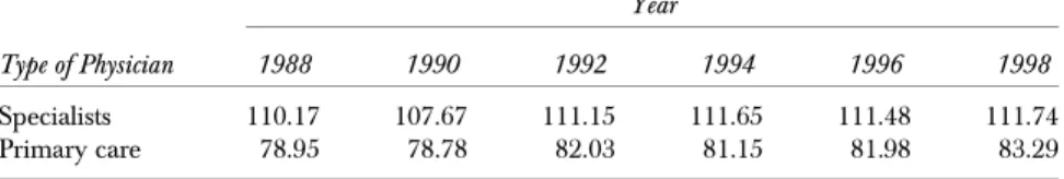
Primary care physicians are defined as physicians who specialize in family practice, general internal medicine, general pediatrics, obstetrics/gyn-ecology, or general practice. Specialists include anesthesiologists, emergency physicians, pathologists, radiologists, internal medicine subspecialists, pe-diatric subspecialists, dermatologists, neurologists, occupational medicine physicians, psychiatrists, rehabilitation physicians, general surgeons, and sur-gical subspecialists. Table 1 presents state-level physician-to-population ratios over time.
County-level estimates of HMO penetration in California’s 58 counties were obtained from Douglas Wholey.5These estimates are preferable to un-adjusted estimates reported by InterStudy, because they correct for errors in reporting HMO enrollment. For the years examined, InterStudy attributes all enrollment to the county in which a HMO is headquartered. Wholey uses an algorithm to annually apportion HMO enrollees across all counties in a
Table 1: Physicians per 100,000 Population in California: 1988–1998
Type of Physician
Year
1988 1990 1992 1994 1996 1998
Specialists 110.17 107.67 111.15 111.65 111.48 111.74
Primary care 78.95 78.78 82.03 81.15 81.98 83.29
HMO’s service area based on county population for the year in question (Wholey, Feldman, and Christianson 1995). Wholey includes only commer-cial HMOs (including Medicaid and Medicare enrollment in these HMOs), but excludes Medicaid-only HMOs in order to focus on commercial HMOs and maintain consistency of the data through time. Table 2 presents state-level and national HMO penetration over time.
Data on other covariates in the model were obtained from the Area Resource File, the California state government, and the Bureau of Economic Analysis. We used these data to construct the following variables: the ratio of county-level real per capita income to real per capita income in the U.S., the percentage of the population enrolled in Medicaid (Medi-Cal in California), hospital beds in short-term hospital per 100,000 population, the percentage of the population that is black, the percentage of the population that is Hispanic, the percentage of the population that is Asian, the percentage of the popu-lation that is below age 18, the percentage of the popupopu-lation that is aged 65 and older, and the percentage of the population that are new legal immigrants in a given year. Data for the exogenous variables in the instrument matrix were obtained from the U.S. Census Bureau’s County Business Patterns.
The means and standard deviations of the variables used are presented in Table 3. As most of the variables listed in Table 3 are ratios, the most
Table 2: Percent of Population Enrolled in HMOs by Year and Geographic Region
Geographic Region
Year
1988 1990 1992 1994 1996 1998
California
Private commercial 28.0 30.0 28.3 30.7 36.2 38.4
Total commercial (including Medicaid and Medicare)n
28.0 30.0 31.6 35.3 42.8 47.6
U.S.
Private commercial 13.1 13.9 14.0 15.8 20.1 23.2
Total commercial (including Medicaid and Medicare)n
13.1 13.9 15.2 17.8 23.5 28.0
Ratio of California to U.S.
Private commercial 2.16 2.16 2.02 1.94 1.80 1.66
Total commercial (including Medicaid and Medicare)n
2.16 2.16 2.08 1.98 1.82 1.70
Source: InterStudy data as adjusted by Douglas Wholey. n
informative information in Table 3 is the standard deviations, which empha-size the wide range of the medical and economic characteristics of California counties. The standard deviations for the physician-to-population ratios are large because of the wide variation in the number of patient care physicians across California’s counties, which ranges from zero in two sparsely populated rural counties to over 15,000 in Los Angeles County.
R
ESULTSSpecification tests of the Arellano–Bond regressions show that the equation is reasonably specified. We estimated both the one- and two-step versions of the Arellano–Bond system estimator. We found the results of the two estimators to Table 3: California County-Level Means and Standard Deviations, 1988– 1998 (n5638)
Variables Meann SD
Yit
Total specialists per 100,000 population 79.470 52.442 Total primary care physicians per 100,000 population 69.100 28.726
Hit
California county HMO penetration to U.S. HMO penetration 1.308 1.052
Iit
Real per capita county income in California to real per capita income in the U.S.
0.931 0.241
Mit
Short-term general hospital beds per 100,000 population 268.969 198.656
Percent population enrolled in Medi-Cal 15.524 6.587
Percent population below age 18 28.044 3.825
Percent population aged 65 and older 12.973 3.683
Percent population black 3.394 3.617
Percent population Hispanic 18.474 13.037
Percent population Asian 5.150 5.749
Percent population that are new legal immigrants Instrumental variables
Percent employees in construction 5.834 2.784
Percent employees in manufacturing 14.400 7.299
Proportion of firms employing 100–249 0.010 0.005
Proportion of firms employing 250–499 0.003 0.003
Proportion of firms employing 5001 0.001 0.003
n
be virtually identical, but found the one-step version slightly more efficient in the present case and so report the one-step results in Table 4.3The Arellano– Bond test for autocorrelation in first differences gives the following results. In
Table 4: Arellano-Bond Regression Estimates
Explanatory Variables
(1) Specialists per 100,000 Population
(2) Primary Care per 100,000 Population
DYiðt1Þ
: specialist physicians per 100,000 populationt1
0.938 ——
(18.64)nn
DYiðt1Þ
: primary care physicians per 100,000 populationt1
—— 0.849
(12.49)nn
DHðt1Þ
: (CA county HMO pen)t1/(U.S. HMO pen)t1
7.278 3.915
(1.93)n (1.00)
DHiðt1ÞIðt1Þ
8.324 4.972
(2.20)n
(1.19) DIiðt1Þ
: (real per capita county income)t1/ (real per capita U.S. income)t1
0.774 4.291
(0.07) (0.53)
DMiðt1Þ: hospital beds per 100,000
populationt1
0.008 0.006
(1.98)n
(1.61) DMiðt1Þ: percent population enrolled in
Medi-Cal
0.143 0.150
(0.78) (0.89)
DMiðt1Þ
: percent population below age 18 0.085 0.212
(0.32) (0.74)
DMiðt1Þ
: percent population aged 65 or older
0.108 0.062
(0.41) (0.28)
DMiðt1Þ
: percent population black 0.165 0.185
(0.49) (0.31)
DMiðt1Þ
: percent population Hispanic 0.011 0.032
(0.16) (0.33)
DMiðt1Þ
: percent population Asian 0.169 0.023
(1.05) (0.07)
DMiðt1Þ
: percent population new legal immigrant
1.840 0.635
(1.18) (0.23)
F-statistic 4948.54nn
2683.71nn
AR(1) (z-statistic) 4.25nn
3.94nn
AR(2) (z-statistic) 1.02 1.53
AR(3) (z-statistic) 1.62 0.38
AR(4) (z-statistic) 0.62 0.50
Hansen’sJstatistic (w2) 52.43 44.41
Levin–Lin–Chu panel unit root test (t-statistic) 3.74nn 16.18nn
Observations 513 513
Number of counties 57 57
Absolute values ofz-statistics in parentheses (two-tailed test). nnSignificant at 1%.
nSignificant at 5%.
columns 1 and 2 of Table 4, which show the specialist and primary care equations, neither second-order autocorrelation (column 1: z5 1.02, p5.31; column 2: z51.53,p5.13), third-order autocorrelation (column 1:z51.62,p5.11; column 2:z50.38,p5.71), nor fourth-order autocorre-lation (column 1: z50.62, p5.54; column 2: z5 0.50, p5.62) are present. These results are consistent with the Arellano–Bond model’s as-sumption of no second-order or higher-order autocorrelation. The results of Levin, Lin, and Chu’s (2002) panel unit root test indicate that we can reject the null hypothesis that the dependent variable is nonstationary (specialist: t53.74,po.01; primary care:t516.18,po.01). In addition, the results of Hansen’sJtest of overidentification (column 1:w2552.43,p5.94; column 2:w2544.41,p5.99) suggest that we cannot reject the null hypothesis that the overidentifying restrictions are valid; that is, we can reasonably conclude that the instrumental variables are not correlated with the error term. We omitted one very small rural county (Alpine county) because it was a statistical outlier. The results show that in the California physician labor market, adjust-ment times vary considerably, but are generally very slow, as can be seen in Table 4. For specialist physicians, the parameter of the lagged dependent variable (D(Yi(t1))50.938,z518.64,po.01) suggests that only (column 1:
10.93850.062) 6.2 percent of the movement towards equilibrium occurs in a given year, which means that it will take (1/0.062516.1) 16.1 years for full adjustment to occur. In other words, the labor market for specialist physicians is, for practical purposes, in continual disequilibrium because of the continual changes in relative HMO penetration and other changes in labor market characteristics. Adjustment times for the primary care physician market are relatively shorter, but still very long. For primary care physicians the param-eter of the lagged dependent variable (D(Yi(t1))50.849, z512.49, po.01)
suggests that (column 2: 10.84950.151) 15.1 percent of the movement towards equilibrium occurs in a given year, which means that it will only take (1/0.15156.62) 6.62 years for full adjustment to occur. Thus, specialists re-spond more slowly than primary care physicians to a given change in market conditions. This difference in the rate at which the two labor markets adjust is consistent with the fact that specialists require much larger market areas than primary care physicians do to sustain a given income.
However, the parameter for relative HMO penetration is negative and sta-tistically significant DðHiðt1ÞÞ ¼ 7:278;z ¼1:93;p¼:05
and the param-eter of the interaction term is positive and statistically significant
DðHðt1ÞÞIðt1ÞÞ ¼8:324;z¼2:20;p < :05
. The linear combination of these two variables at the mean values of the differenced variables is 0.114 (z52.52,p5.01) indicating their average negative effect on spe-cialist migration. This finding is consistent with our conceptual framework. We do not find any statistically significant results on these key variables for primary care physicians, which is also consistent with our conceptual frame-work.
However, this does not imply that there are no circumstances in which the relative economic environment cannot dominate the effect of changes in relative HMO penetration. The above discussion only describes the mean effect. Different situations will result in different effects on specialist migration. For example, if the relative economic environment is 50 percent better in a county relative to the U.S. average, an increase in relative HMO penetration of 1.0 is associated with the migration of specialists migration into such a county (column 1: (8.3241.5)7.27855.21,z52.50,p5.01). This effect is stronger, the more favorable the relative economic environment is. In fact, it appears that this reversal occurs whenever the relative economic environment is favorable by 5 percent or more (column 1: (8.3241.05)7.27851.46, z51.97,p5.05).
The signs of the remaining parameters are all reasonable. The effect of lagged increases in short-term general hospital beds per 100,000 population is slightly negative and statistically significant DðMiðt1ÞÞ ¼ 0:008;
z¼1:98;p < :05Þ. This is to be expected as there was a consolidation of
the hospital market during this period with many hospitals or hospital services closing (Lindrooth, Lo Sasso, and Bazzoli 2003; Kirby et al. 2005). From 1988 to 1998 the number of short-term general hospital beds per 100,000 popu-lation in California declined by 22.4 percent. Thus, while the parameter values make it appear as if physicians were moving away from areas with lagged growing numbers of hospital beds, a more plausible explanation is that hos-pital beds were being reduced in the urban areas that physicians prefer.
Hispanic, the percentage of the population that is Asian, and the percentage of the population that are new legal immigrants in a given year.6
D
ISCUSSIONOur findings augment the conventional wisdom that growth in relative HMO penetration has led to a redistribution of physicians away from areas with high rates of growth in relative HMO penetration. Our results suggest that the relationship between changes in relative HMO penetration and phy-sician stock is more complex than previously thought, with differences in the relative economic environment being important moderators of the effect of changes in relative HMO penetration. Our use of a dynamic panel estimator enables us to detect short-run changes that were not assessed in previous studies.
Further research is needed to determine the impact of changes in relative HMO penetration and the relative economic environment by physician age. The number of patient care physicians in California age 40 or younger has decreased in California counties even though the total number of physicians has increased. (Results not shown.) The likelihood that changes in relative HMO penetration and the relative economic environment play a role in be-havior of young physicians is supported by the findings of both Escarce et al. (1998) and Polsky et al. (2000).
Escarce et al. (1998) examined physician migration using national data for the years 1989–1994 on young patient-care physicians. They found that young generalist physicians were more likely than young specialist physicians to establish their initial practice in areas with high HMO penetration. They also found that the probability of locating in an area with high HMO pen-etration relative to low penpen-etration areas decreased over time for both gen-eralists and specialists. Whether this was because of decreased opportunities for both types of physicians in high HMO penetration areas or because of changing physician preferences regarding working in high HMO penetration areas (or both) was unclear, but indirect evidence suggested that tightening labor markets may have been be responsible for the change.
mid-career medical/surgical specialists. They also found that physicians who relocated tended to move to areas with the same or lower HMO penetration. Our findings are likely to be of interest to policymakers concerned about issues of physician supply and distribution. While it appears as if HMO pen-etration does affect physician supply, it does not drive away specialist phy-sicians in all cases. The business cycle and the relative economic environment are important factors to consider. As a result, it is important to consider the possibility that policies made during relatively bad economic times may have very different effects once the relative economic environment improves. Our finding also suggests that economic development may be a useful strategy for improving access to care in underserved areas.
A
CKNOWLEDGMENTSWe express our great appreciation to Douglas R. Wholey, Ph.D., for the permission to use his HMO penetration data. We also thank our editors, Ann B. Flood and Jose´ J. Escarce, and two anonymous reviewers for their valuable input. This work was supported by the Nicholas C. Petris Center for Health Care Markets and Consumer Welfare, School of Public Health, University of California, Berkeley.
N
OTES1. An additional study (Waitzman and Scheffler 1992) found that in 1990, internists in markets with low rates of HMO penetration had fees that were 11.6 percent lower than fees in markets with no HMO penetration, and that internists in markets with medium levels of HMO penetration had fees that were 16.9 percent lower. How-ever, the reductions were much less pronounced in markets with high rates of HMO penetration. Waitzman and Scheffler’s results are difficult to compare with those of other studies because their sample does not permit them to disaggregate general internists from medical subspecialists.
2. Using OLS to estimate dynamic panel models is well known to result in biased and inconsistent estimates. Anderson and Hsiao (1981, 1982) have developed an es-timator that addresses the problems that arise with OLS by taking first differences and instrumenting the lagged dependent variable using either lagged levels or lagged differences of the dependent variable. This method yields consistent es-timates but is inefficient because it does not use all the available moment restric-tions (Arellano and Bond 1991).
of all of the variables included in the main regression (less interaction terms) as ‘‘GMM-style’’ instruments. To make sure we included all appropriate variables as instruments, but to avoid biasing our parameters, we used the ‘‘collapse’’ option and thus only included one instrument for each variable and lag distance rather than one instrument for each variable, time period, and lag distance. This was done because as the number of instruments included becomes large relative to sample size, the parameter estimates will become biased towards feasible GLS. The ratio of instruments to observations in our model is only 0.16. We used a generalized inverse to calculate the robust weighting matrix when using two-step estimation. Two-step results were virtually identical to one-step results, with the one-step re-sults being slightly more efficient (slightly smaller standard errors for the main variables of interest,DHiðt1ÞandD Hiðt1ÞIðt1Þ
, with both versions finding sta-tistically significant results for these variables in the specialist equation.
4. The AMA did not collect data for the year 1990. We interpolated the values for 1990 by taking the arithmetic mean of 1989 and 1991.
5. We would like to express our great appreciation to Dr. Douglas Wholey for the permission to use these data.
6. In the present case our data are not a sample of physicians from California coun-ties, but the universe. Some argue that in the case where the data being analyzed are the universe rather than a sample from the universe, computing confidence intervals in order to determine how likely the parameter of the sample is to ap-proximate the parameter of the universe is inappropriate (McCloskey 1985; McC-loskey and Ziliak 1996). In this alternative view, when using a universe rather than a sample, all of the estimated parameters would be used to determine the results rather than the statistically significant parameters alone.
REFERENCES
Anderson, T. W., and C. Hsiao. 1981. ‘‘Estimation of Dynamic Models with Error Components.’’Journal of the American Statistical Association76 (375): 598–606. ——————. 1982. ‘‘Formulation and Estimation of Dynamic Models Using Panel Data.’’
Journal of Econometrics18: 47–82.
Arellano, M., and S. Bond. 1991. ‘‘Some Tests of Specification for Panel Data: Monte Carlo Evidence and Application to Employment Equations.’’The Review of Eco-nomic Studies58 (2): 277–97.
Arellano, M., and O. Bover. 1995. ‘‘Another Look at the Instrumental Variable Es-timation of Error-Components Models.’’Journal of Econometrics68: 29–51. Baltagi, B., E. Bratberg, and T. H. Holmas. 2005. ‘‘A Panel Data Study of Physicians’
Labor Supply: The Case of Norway.’’Health Economics14: 1035–45.
Blundell, R., and S. Bond. 1998. ‘‘Initial Conditions and Moment Restrictions in Dy-namic Panel Data Models.’’Journal of Econometrics87: 115–43.
Escarce, J. J., D. Polsky, G. D. Wozniak, and P. R. Kletke. 2000. ‘‘HMO Growth and the Geographic Redistribution of Generalist and Specialist Physicians, 1987–1997.’’
Health Services Research35 (4): 825–48.
Hadley, J., and J. M. Mitchell. 1999. ‘‘HMO Penetration and Physicians’ Earnings.’’
Medical Care37 (11): 1116–27.
——————. 2002. ‘‘The Growth of Managed Care and Changes in Physicians’ Incomes, Autonomy, and Satisfaction, 1991–1997.’’International Journal of Health Care Fi-nance and Economics2 (1): 37–50.
Jiang, H. J., and J. W. Begun. 2002. ‘‘Dynamics of Change in Local Physician Supply: An Ecological Perspective.’’Social Science and Medicine54 (10): 1525–41. Kirby, P., J. Spetz, L. Simonson-Mairuo, and R. Scheffler. 2005. ‘‘Hospital Service
Changes in California: Trends, Community Impacts and Implications for Pol-icy.’’ Nicholas C. Petris Center on Health Care Markets and Consumer Welfare [accessed May 19, 2005]. Available at http://www.petris.org/docs/california-hospitals.pdf
Levin, A., C. F. Lin, and C. S. J. Chu. 2002. ‘‘Unit Root Tests in Panel Data: Asymptotic and Finite Sample Properties.’’Journal of Econometrics108: 1–24.
Lindrooth, R. C., A. T. Lo Sasso, and G. J. Bazzoli. 2003. ‘‘The Effect of Urban Hospital Closure on Markets.’’Journal of Health Economics22 (5): 691–712.
Mark, B. A., D. W. Harless, M. McCue, and Y. Xu. 2004. ‘‘A Longitudinal Exam-ination of Hospital Registered Nurse Staffing and Quality of Care.’’Health Serv-ices Research39 (5): 1629.
McCloskey, D. N. 1985. ‘‘The Loss Function Has Been Mislaid: The Rhetoric of Significance Tests.’’American Economic Review75: 201–5.
McCloskey, D. N., and S. T. Ziliak. 1996. ‘‘The Standard Error of Regressions.’’Journal of Economic Literature34: 97–114.
Newhouse, J. P., A. P. Williams, B. W. Bennett, and W. B. Schwartz. 1982. ‘‘Does the Geographical Distribution of Physicians Reflect Market Failure?’’Bell Journal of Economics13 (2): 493–505.
Polsky, D., P. R. Kletke, G. D. Wozniak, and J. J. Escarce. 2000. ‘‘HMO Penetration and the Geographic Mobility of Practicing Physicians.’’Journal of Health Eco-nomics19 (5): 793–809.
Simon, C. J., D. Dranove, and W. D. White. 1997. ‘‘The Impact of Managed Care on the Physician Marketplace.’’Public Health Reports112 (3): 222–30.
——————. 1998. ‘‘The Effect of Managed Care on the Incomes of Primary Care and Specialty Physicians.’’Health Services Research33 (3, part 1): 549–69.
Waitzman, N. J., and R. M. Scheffler. 1992. ‘‘The Effects of HMO Penetration on Physician Fees: Evidence on Primary Care Physicians in 1990.’’L’e´volution des syste´mes des sante´.
Wholey, D., R. Feldman, and J. Christianson. 1995. ‘‘The Effect of Market Structure on HMO Premiums.’’Journal of Health Economics14 (1): 81–105.