TECHNICAL UNIVERSITY OF CLUJ-NAPOCA
ACTA TECHNICA NAPOCENSIS
Series: Applied Mathematics, Mechanics, and Engineering Vol. 63, Issue I, March, 2020
CALIBRATION PROCEDURE FOR PENDULUM POSITION
MEASUREMENT
Ioan CIASCAI, Adrian MOCAN
Abstract: A calibration procedure for pendulum movement is described. Such a pendulum is used in the monitoring structural integrity of dams. The movement detection of the pendulum is made with an optoelectronic measurement instrument. The calibration procedure uses a lot of measurements taken for reference positions in a grid pattern. For each reference position multiple measurements are taken with different LEDs. An algorithm that interpolates the grid measurements is presented. The algorithm solves the problem that arises when between two grid measurements another LED is used. This changing of LED between two grid points may introduce discontinuities that affects the interpolation. The presented algorithm makes the interpolation without being affected by the changing of LED.
Keywords: calibration, pendulum, dam, measurement, grid, optical.
1. INTRODUCTION
We researched a method for the calibration of an instrument used to detect the small movement of a pendulum. Such a pendulum is used in the monitoring structural integrity of dams. The instrument makes continuous measurements of the position of the pendulum wire by detecting the shadow cast by the pendulum on an optical sensor when the light source is an LED. The optical sensor consists in an array of photodetectors arranged in a line with a distance of 63.5μm[1] between them.
Fig. 1. Measurement principle of the instrument
To make a measurement two LEDs are selected from a band of LEDs. They are turn on,
each of them in turn. Knowing LEDs positions and then reading the position of the pendulum shadow casted on the optical sensor is possible to determine the pendulum position. The measurement principle can be seen in Fig. 1.
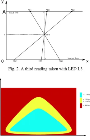
In order to find the pendulum position with a better accuracy, the LEDs are turned on in turns, starting from the ends of the LED band and progressing towards the middle, until a shadow of the pendulum is cast on the optical sensor. In this way is possible to find the greatest distance between the LEDs and the greatest distance between the shadows. This configuration gives the smallest errors. A third reading will be made with an LED selected to match the position of the newly computed x, so that the light ray should be closest to perpendicular to the optical sensor, see Fig. 2.
the y coordinate of wire position when no calibration is made for the LEDs positioning.
Fig. 2. A third reading taken with LED L3
Fig. 3. Errors for the y coordinate of the wire when no calibration is used for the LED positioning
Also, for the big incidence angle of the light ray, refraction[3] in LED and optical sensor can cause big measurement errors.
To reduce these errors, we want to find a calibration procedure that will reduce the errors due to LEDs positioning, the errors due to refraction, and other type of systematic errors.
For calibration we want to use a simulated pendulum that can be positioned very precisely. We use this positioning as a reference for the measurement. To achieve the reference positioning we used a system of stepper motors with micro-stepping that can give a positioning accuracy of 5μm.
At first we have tried to calibrate only the LEDs position by using the reference position and the shadow position. By having a good accuracy for both the reference and shadow positon, the LED position can be determined with an improved accuracy. This improved
accuracy for the LED position can be stored and then used to improve the measurement accuracy of the instrument. Working with this approach we discovered that refraction is another source of errors [4] that we need to compensate also. We want to improve on that approach, so we decided to go for a calibration procedure that will be applied globally for the whole instrument and it will address all the systematic error sources so that we have the best accuracy for the instrument.
2. CALIBRATION METHOD
The instrument calibration starts by taking several measurements with the simulated wire positioned in certain reference points and then store the sensor readings in a table. We want to find a method with which we can use the data from this table to measure with the best accuracy any position of the wire.
We will call in this paper “reading” a value read from the optical sensor for the position of the shadow casted by a wire, when an LED is turned ON. Also we will call “position”, the x and y coordinates of the wire for which we measure its position. Coordinates x and y are relative to the optical sensor so that the coordinate 0,0 will be at the pixel 0 of the optical sensor and the x axis will go along the pixel array in the optical sensor [1].
A first approach to make a global calibration procedure was to make the measurements for a grid of very accurate positions and store in a table the difference between the reference position and the position given by the theoretical mathematical equation of the instrument. Knowing these differences for each point in the grid, at an intermediary point we can estimate the difference between the real position and the position obtained through the mathematical equation of the instrument by using a bilinear interpolation of the differences in the grid. By adding this interpolated difference to the theoretical position given by the measurement equation of the instrument we can obtain a better accuracy for the measurements of the instrument. Unfortunately there is a problem that precludes the use of this method. For different wire positions the LED used needs to be changed
x L3 xL2
x L1
x S3 x S1
x x
xS2
sensor lin e w ire
LEDs line
y
so that the LEDs that gives the smallest errors are used. Changing the LED between two points of the grid that needs to be interpolated can cause discontinuities that will affect the interpolation result.
To avoid this type of errors that are given by the changing of LEDs for different positions of the wire, we seek to make measurements in the grid with all the LEDs that gives valid readings on the optical sensor and to store all of these readings in reading tables for each LED. We search then for a method with which we can use the readings from these tables to increase the measurement accuracy for any position in the measurement field.
When a new position is measured with the instrument we would like to know which is the closest point on the grid to this new position we try to measure. For this grid point we have a very accurate position from reference measurements. For the new position measurement we have two readings from the optical sensor and with these two readings we want to determine the distance from the new measurement to a grid point. We suppose that the grid point is close to the position we want to measure, so we can use the values from the tables of the same two LEDs that were used for the measurement. We will call those two positions of the wire Position 0 and Position 1. Position 0 is a reference position, from the grid so we have for the Position 0 the values of readings taken from tables. Position 1 is the position we want to measure and for this position we have only the two readings from the optical sensor.
Fig. 4. Find coordinates where light ray crosses the axes with the origin in Position 0
First we compute dwx and dwy, the
coordinates where the light ray crosses the x and y axes when the axes origin is located in the Position 0, see Fig. 4.
From similar triangles we can write the equations:
= − (1)
= (2)
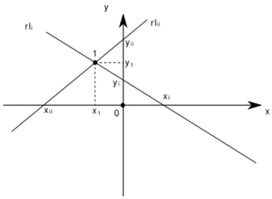
Having the two readings for Position 1 we can compute the coordinates for each reading so that we have four points on the axes. The four points determines two lines that models the two light rays. By finding the intersection point of the two lines we find the coordinates of the position 1 relative to Position 0. To simplify the calculation we took here the origin of the x and y axes in the Position 0, see Fig. 5.
Fig. 5. Find coordinates for Position 1 relative to Position 0
We call the two readings Reading i and Reading ii. We will have then the coordinates where the light rays crosses the axes for the two readings: xi=dWx, yi=dWy for Reading i,
xii=dWx, yii=dWy for Reading ii. The
coordinates for the lines intersection point[5] i.e. coordinates of Position 1 relative to Position 0 are:
= (3)
= (4)
x y
xL xW0 xS0 xS1
0 1 LED
dS dWx dWy yW0
yL
x y
0 1
r li r lii
xi yi
yii
xii
y1
The distance between Position 0 and Position 1 will be then:
= + (5)
From equations 1,2,3,4 and 5 is possible to compute the distance between a position we want to measure and a known position from the grid. For this known position we have the readings from the tables and we also use in the computation the readings for the position we want to measure. In fact we have already determined Position 1 when we computed x1 and
y1, but we want to determine Position 1 with a
better accuracy. To have a better accuracy when computing Position 1 we will use an interpolation algorithm.
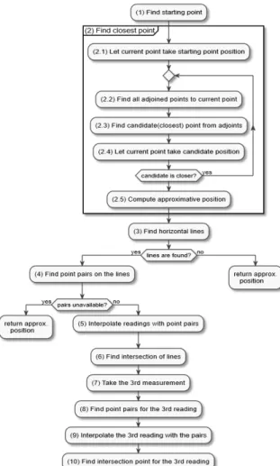
The interpolation algorithm used to find a measured position is presented below, see Fig. 6.
Fig. 6. Grid interpolation
1. Find a starting point in the grid. It will be a point close to the theoretical position given by the geometric method[2]. From this starting point we start spiraling outwards until we find the first grid point that has valid readings on both LEDs.
2. We find the grid point with valid reading for both LEDs that is closest to the position we try to measure.
2.1. We take as current point the point found at step 1.
2.2.We find all the adjoined grid points to the current point that have valid readings on both LEDs.
2.3.For each point found at step 2.2, we compute the distance to the position to measure and we take as candidate point the one with the minimum distance.
2.4. If the candidate point have the distance less than the current point, it became the new current point and we go to step 2.2. Otherwise the current point will be the closest grid point to the position to be measured.
2.5. We compute the coordinates of the position to be measured relative to the closest grid point and we retain this position as the less accurate alternative. We will use this less accurate position and use it where the interpolation cannot be computed because there are not enough valid points.
3. We find two horizontal lines in the grid that are closest to the position to be measured. If the two lines cannot be found the approximate position computed on step 2.5 is returned.
4. For each of the horizontal lines we find a pair of grid points that are closest to the point where the light ray crosses the horizontal line. If two points cannot be found for each light ray crossing, the approximate position computed on step 2.5 is returned.
5. For each point pair found at step 4 we apply a procedure of linear interpolation by finding the x coordinate between the two grid points that corresponds to the sensor reading.
6. With the four points found at step 5 we determine the position to be measured as the intersection point of the two lines given by the founded points. The two lines gives a good approximation of the light rays from the two LEDs.
7. From the x coordinate of the position to be measured we take the closest LED and make one more reading by turning on this LED. This 3rd reading will improve the accuracy
on the x axis[2].
x
8. On the two horizontal grid lines we find two pair of grid points that are closest to the light ray from 3rd LED.
9. We find a point on each horizontal grid line through interpolation of the reading with the grid point pair found at step 8.
10.We find a more accurate value for x coordinate at the intersection of the line given by the 2 points found at step 9 with the horizontal line given by the y coordinate found at step 6.
The visual structure of the algorithm is presented in Fig. 7.
Fig. 7. Diagram of the algorithm
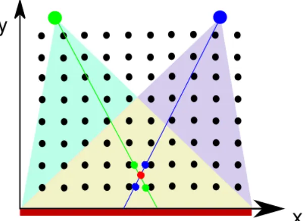
This algorithm may have a problem when the position to be measured is close to the margin of the measurement field of an LED. It can be seen on Fig. 8 such a case that is not a good fit for the interpolation procedure. For the LED
represented with the green color, on the grid line above the position to be measured there is only one valid reading in the grid. In such a case we will return with the position computed with relations (3) and (4) relative to the closest grid point (represented with turquoise color in Fig. 8), where we have valid readings for both LEDs. Although is not as accurate as a position obtained through interpolation, the value for the position computed with (3) and (4) is based on a reference value from the grid and so is more accurate than a position determined purely geometrically without taking in consideration the positioning errors of LEDs and the refraction errors.
Fig. 8. Grid interpolation in a degenerate case
3. CONCLUSIONS
The presented calibration procedure can be applied for this type of position measuring instrument that uses optoelectronic methods. This calibration procedure uses many measurements taken as reference points and uses an algorithm capable of doing interpolation of the readings even when readings for interpolation are taken with a different LEDs. This method was developed to improve the measurement accuracy of this type of instrument compared with other calibration methods[4], [6]. This calibration method uses many reference measurements which is a time consuming activity, so is better suited for instruments produced in smaller quantities.
x
4. REFERENCES
[1] TAOS Inc., TSL1412S 1536 × 1 LINEAR
SENSOR ARRAY WITH HOLD,
TAOS045F, Apr. 2007, https://html.alldatasheet.com/htmlpdf/20 3049/TAOS/TSL1412S/97/1/T
SL1412S.html
[2] Mocan A. and Ciascai I., A model for measuring the position of a pendulum
using opto-electronic method, Acta
Technica Napocensis, Series: AMME, Issue IV, Vol. 61, 2018
[3] Peatross J. and Michael W., Physics of
Light and Optics, Lulu, 2015, ISBN
9781312929272.
[4] Mocan, A., Ciascai, I., Analysis of
positioning errors for LED, 2019 IEEE
25th International Symposium for Design and Technology in Electronic Packaging (SIITME), pp. 127-130, ISBN 978-1-7281-3330-0, Cluj-Napoca, Romania, 2019.
[5] Wikipedia, Line–line intersection,
https://en.wikipedia.org/wiki/Line– line_intersection#Given_two_points_on_ each_line.
[6] Pop S., Ciascai I., Bande V. and Pitica D.,
Modeling the light of LED’s for position
detection with an optical sensor, in 33rd
International Spring Seminar on Electronics Technology, ISSE 2010, pp. 374–377.
PROCEDURĂ DE CALIBRARE PENTRU MĂSURAREA POZIȚIEI UNUI PENDUL
Rezumat: Se descrie o metodă de a calibra un instrument opto-electronic de măsură a deviației unui pendul de monitorizare a barajelor. Procedura de calibrare folosește multe măsurători luate într-un grid de poziții, pentru fiecare poziție folosind LED-uri diferite. Se prezintă un algoritm care face o interpolare a valorilor din grid. Algoritmul prezentat rezolvă situația în care între măsurători alăturate se schimbă LED-ul cu care se face măsurătoarea și se introduc astfel discontinuități in domeniul de măsură.
Ioan CIASCAI, Professor Ph.D., Technical University of Cluj-Napoca, Department of Applied Electronics, 24-26 George Baritiu str. 400027 Cluj-Napoca, +40-264-401809, e-mail:
Adrian MOCAN, drd., Technical University of Cluj-Napoca, Department of Applied Electronics, 24-26 George Baritiu str. 400027 Cluj-Napoca, +40-723-873249, e-mail: