1. Introduction. 2. Key Findings

COMPARISON OF TRANSPORTATION OPTIONS

IN A CARBON-CONSTRAINED WORLD:

HYDROGEN, PLUG-IN HYBRIDS AND BIOFUELS

By C. E. (Sandy) Thomas, Ph.D.*

National Hydrogen Association Annual Meeting

Sacramento, California, March 31, 2008

1.

Introduction

Most automobile and energy company executives, academics and government planners acknowledge the long-term promise of hydrogen-powered fuel cell vehicles (FCVs). Some organizations are now promoting plug-in hybrid electric vehicles (PHEVs), and biofuels such as ethanol or butanol. These near-term options are desirable and should be pursued to reduce our demand for imported oil, but they should not be taken as a substitute for much better mid- to long-term solutions to curb urban air pollution, climate change gases and oil consumption. The national security and environmental imperatives for action are so strong that we should be vigorously pursuing all plausible transportation alternatives without delay.

We have developed an extensive computer model to simulate the societal benefits of various alternative transportation options including hybrid electric vehicles (HEVs) and plug-in hybrids fueled by gasoline, diesel fuel, ethanol and hydrogen, including both internal combustion engines (ICEs) and fuel cell (FC) power sources. These simulations compare the societal benefits of each vehicle/fuel combination in terms of reduced local air pollution, reduced greenhouse gas pollution, and reduced oil consumption.

2.

Key Findings

The major conclusions from these computer simulations are:

Greenhouse gas reductions: the hydrogen-powered fuel cell vehicle is the only option

that could achieve the goal of reducing GHGs by 80% or more below 1990 levels in the transportation sector; the second-best option, hydrogen-powered ICE HEVs could reduce GHGs to 60% below 1990 levels; cellulosic ethanol1 PHEVs, could at best achieve a 25% reduction, and even then not until 2090; battery EVs might reach a 60% reduction by 2100.

Urban air pollution: the hydrogen-powered fuel cell vehicle is the only option that

would nearly eliminate all controllable2 urban air pollution from the transportation sector by 2100; all other vehicle/fuel options including both gasoline and ethanol PHEVs would produce essentially the same or greater urban air pollution as the existing car fleet due to increased vehicle miles traveled.

1 _{Existing corn ethanol could not even reach this level of GHG reduction.} 2 _{Particulate emissions from brake & tire wear continue for all vehicles.}

3 _{“Quasi-independence” is defined here as reducing oil consumption in the transportation sector to the level that} US domestic oil production could supply all petroleum needs in a crisis, assuming no growth in non-transport oil consumption and no further decline in US oil production capacity.

ethanol PHEVs would still consume over 5 million barrels of oil per day by the end of the century.

Hydrogen infrastructure

:

Societal cost savings5: hydrogen-powered fuel cell vehicles will provide greater societal cost savings than any other alternative: each FCV sold will cut societal costs by a factor of 7.8 relative to conventional gasoline cars in the near-term (now to 2020), by a factor of 10.7 in the mid-term (2021 to 2050) and by a factor of 20.4 in the long-term (2051 to 2100); second-best option is the hydrogen-powered ICE HEV (reduction factors of 5.1, 6.6, 13.2); third-best the battery EV (4.2, 4.6, 10.6); fourth-best the ethanol plug-in hybrid (3.8, 4.8, 6.8) and fifth-best the gasoline plug-in hybrid (1.7, 2.1, 2.9) (See Figure 7 below).

3.

Basis of Key Findings

We have focused on five vehicle/fuel scenarios to illustrate our key findings:

• Reference Case: 100% gasoline ICEVs

• Base Case: Gasoline HEV Scenario (including gasoline ICEVs) • Gasoline PHEV Scenario (including gasoline ICEVs and HEVs)

• Cellulosic Ethanol PHEV Scenario (including gasoline ICEVs and HEVs) • Hydrogen FCV Scenario (including all of the above in the early years)

3.1.

Greenhouse gas results

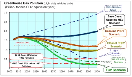
Figure 1 shows the projected greenhouse gas emissions from the four main scenarios plus three reference cases (100% conventional gasoline ICEVs (no hybrids of any kind), hydrogen ICE HEVs and BEVs). In the base case with gasoline HEVs, GHGs are reduced from the

4 _{Incentives or feebates will most likely be required, however, to reduce the initial FCV costs}

5 _{Societal costs include the health costs of urban air pollution, greenhouse gas emissions (varying linearly from} $25/metric tonne of CO2 in 2010 to $50/tonne in 2100) and the added societal costs of oil consumption (taken as $60/barrel; this societal cost is not the price paid for oil)

Figure 1. Greenhouse gas emissions for the four main scenarios plus three reference cases Story Simultaneous.XLS; Tab 'Graphs'; AN 344 6/24 /2008

-0.5 1.0 1.5 2.0 2.5 3.0 2000 2010 2020 2030 2040 2050 2060 2070 2080 2090 2100

Greenhouse Gas Pollution (Light duty vehicles only) (Billion/ tonnes CO2-equivalent/year)

1990 LDV GHG Level GHG Goal: 60% below 1990 Pollution GHG Goal: 80% below 1990 Pollution FCV Scenario Ethanol PHEV Scenario Gasoline PHEV Scenario PHEVs Base Case: Gasoline HEV Scenario 100% Gasoline ICEVs H2 ICE HEV Scenario BEV Scenario

reference case, but continue to rise through the century. The climate change goals of reducing GHGs to 60% or 80% below 1990 levels6 are also shown at the bottom of Figure 1 for light duty vehicles. With the assumptions in this model, the fuel cell vehicle is the only scenario to achieve reductions of 80% below

1990 levels; the (cellulosic) ethanol PHEV cuts GHGs 25% below 1990 levels. Without substantial ethanol use, the gasoline PHEV would return GHGs to 5% below 1990 levels by 2100, and GHG pollution would increase for both PHEVs after 2090 as vehicle miles traveled continued to rise.

3.2.

Urban air pollution

results

The FCV is the only main alternative that would substantially reduce urban air pollution according to the Argonne GREET model.

3.3.

Oil consumption results

The horizontal line near the bottom of Figure 3 labeled energy “quasi-independence” is the level where the projected US oil production of 7.5 million barrels/day in 2030 could meet all non-transportation needs (6.2 Mbbl/d, assuming no growth), leaving 1.3 Mbbl/d (or 0.5 billion barrels/year on the graph) for transportation needs. Only the FCV among the four main alternatives achieves this quasi-energy independence (by 2060); battery EVs and hydrogen ICE HEVs would also achieve this objective.

3.4.

Hydrogen infrastructure cost results

The model calculates the cost of installing a distributed hydrogen infrastructure based on steam methane reforming of natural gas, using data from the DOE H2A cost model. The total hydrogen infrastructure costs reach more than $35 billion per year by the end of the century.

6 _{Senate Bill S.280 sets goal of 60% reduction below 1990 GHG levels by 2050; Senate Bill S.309 sets a goal of} 80% below 1990 levels by 2050, and the states of California, Florida and Minnesota have enacted goals of 80% reduction by 2050, while New Mexico and Oregon has enacted 75% reductions by 2050.

Figure 3. Petroleum consumption projections for the alternative vehicle scenarios, including the estimated oil consumption level such that US domestic production could supply all non-transportation petroleum requirements. Figure 2. Urban air pollution costs (sum of grams/mile for each pollutant times $/kg societal cost) for each scenario; the lower line shows the costs for the health effects of particulates from brake & tire wear

-1.0 2.0 3.0 4.0 5.0 6.0 7.0 8.0 2000 2020 2040 2060 2080 2100 Oil Consumption (Billion barrels/year) FCV, H2 ICE PHEV & BPEV

Scenarios Gasoline PHEV Scenario PHEVs Ethanol PHEV Scenario Base Case: Gasoline HEV Scenario 100% Gasoline ICEVs Energy "Quasi-Independence" -10 20 30 40 50 60 70 80 2000 2020 2040 2060 2080 2100 FCV Scenario Ethanol PHEV Scenario Gasoline PHEV Scenario Base Case: Gasoline HEV Scenario 100% Gasoline ICEVs US Urban Air Pollution Costs

($Billions/year)

H2 ICE HEV Scenario

BPEV Scenario

However, as shown in Figure 4, these costs are minimal compared to what the oil and gas industry spends today to maintain the existing gasoline and diesel fueling system.

These costs are also similar to the $35 to $40 billion per year that will be required to reduce utility grid GHG pollution to at least 60% below 1990 levels (See Figure 13 below).

3.5.

Societal cost savings

results

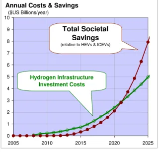
The model also calculates the total societal cost savings relative to the base case of gasoline ICEVs and HEVs from reducing urban air pollution, reducing greenhouse gases, and reducing oil consumption. These societal savings exceed the hydrogen infrastructure costs by 2022, rising rapidly thereafter as shown in Figure 5 for the near-term, and in Figure 6 for the long-term. These graphs only refer to the costs of installing and maintaining a hydrogen infrastructure and do not address any incentives to offset the extra cost of the FCVs during early deployment.

The model sums the costs of urban air pollution, greenhouse gas emissions and oil consumption for each alternative vehicle/fuel combination. We then calculate a cost reduction factor, defined as the total societal costs attributed to a conventional gasoline (non-hybrid) car divided by the total societal costs of the alterative vehicle. These cost reduction factors change as the electrical grid and the sources of ethanol and hydrogen become greener over time. Figure 7 shows these cost reduction factors for each

vehicle type averaged over three time periods: near-term (now to 2020), mid-term (2021 to 2050) and long-term (2051 to 2100).

Figure 4. Projected hydrogen infrastructure costs compared to estimated costs of maintaining the current US gasoline and diesel fueling system

Figure 5. Projected near-term costs of a distributed hydrogen fueling system compared to the projected societal savings

H2 Energy Story.XLS; Tab 'Annual Sales';ID 146 5/25 /2008

0 20 40 60 80 100 120 140 160 180 200 2000 2005 2010 2015 2020 2025 2030

Annual US Fuel Infrastructure Capital Expenditures

($US Billions)

Projected Hydrogen On-Site Infrastructure

Expenditures

Current Energy Company Expenditures in US

Estimated Capital Expenditures on Gasoline & Diesel

H2 Energy Story.XLS; Tab 'Annual Sales';FY 25 6/24 /2008 0 1 2 3 4 5 6 7 8 9 10 2005 2010 2015 2020 2025

Annual Costs & Savings

($US Billions/year)

Hydrogen Infrastructure Investment Costs

Total Societal Savings (relative to HEVs & ICEVs)

PM-10 PM-2.5 SOx VOC CO NOx CO2

Costs of Pollution: 1,608 134,041 29,743 6,592 1,276 13,844 25 to 50

($/metric tonne) Crude Oil Economic Cost $60/bbl H2 Energy Story.XLS; Tab 'Annual Sales';FL 26 5/25 /2008

0 50 100 150 200 250 300 350 400 450 500 550 600 650 2000 2010 2020 2030 2040 2050 2060 2070 2080 2090 2100

Total Societal Savings

(relative to ICEVs)

Annual Costs & Savings

($US Billions/year)

Hydrogen Infrastructure Investments

Total Societal Savings

(relative to HEVs & ICEVs)

Hydrogen FCV Scenario

Figure 6. Long-term projections of the hydrogen infrastructure costs compared to the total societal savings from deploying FCVs in terms of reduced urban air pollution, reduced greenhouse gases and reduced oil consumption with the costs listed above; the FCV would save more than $400 Billion per year compared to HEVs, and over $600 Billion per year compared to ICEVs by the end of the century.

We now turn to the assumptions and details behind these results.

4.

Vehicles & Fuels

Considered

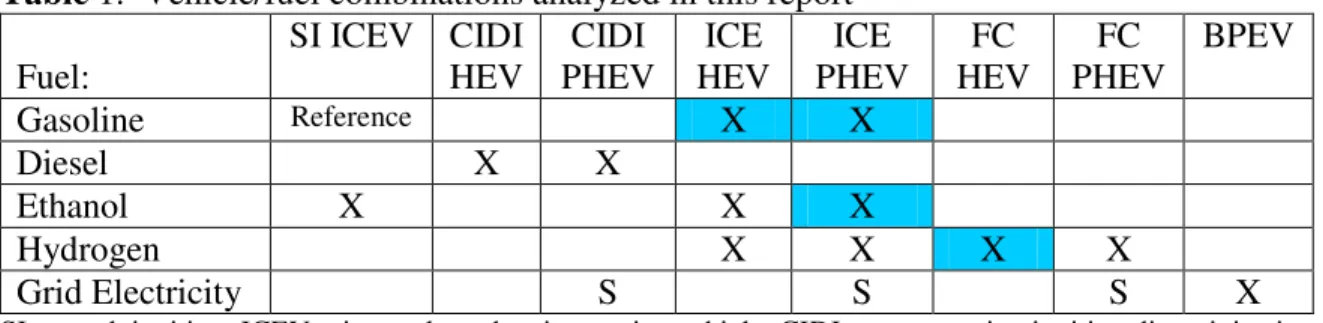
We considered eight types of vehicle and five different fuels and analyzed in detail 12 different alternative vehicle/fuel combinations plus the gasoline ICEV reference case (Table 1). These alternatives represent vehicle/fuel combinations that have the best chance (or are being promoted as having a good chance) of achieving our transportation goals of reduced environmental and oil footprints.

Figure 7. Societal cost reduction factors for alternative vehicle/fuel combinations over three time periods: near-term (now to 2020), mid-near-term (2021 to 2050) and far-term (2051 to 2100)

Summary Greet 1.8a.XLS; Tab 'Summary'; AG 200 4/21 /2008

-2 4 6 8 10 12 14 16 18 20 22 FCV H2 ICE PHEV

BPEV EtOH PHEV Gasoline PHEV Gasoline HEV Near-Term Mid-Term Far-Term Total Societal Cost Reduction Factor per Vehicle

Detailed dynamic simulations were run for the four highlighted vehicle/fuel combinations7. Table 1. Vehicle/fuel combinations analyzed in this report

Fuel: SI ICEV CIDI HEV CIDI PHEV ICE HEV ICE PHEV FC HEV FC PHEV BPEV Gasoline Reference _{X X} Diesel X X Ethanol X X X Hydrogen X X X X Grid Electricity S S S X

SI = spark ignition; ICEV = internal combustion engine vehicle; CIDI = compression ignition direct injection; PHEV = plug-in hybrid electric vehicle; FC = fuel cell’ BPEV = battery-powered electric vehicle; X= primary fuel; S = Secondary fuel for PHEVs

5.

Study Methodology

For each vehicle/fuel combination, we calculated the local air pollution (VOCs, NOx, CO, SOx, PM-2.5, PM-10), greenhouse gas (GHG) emissions and oil consumption using the GREET computer model developed by Michael Wang and associates at the Argonne National Laboratory [1]. We modified some of the GREET default input parameters over time to reflect the changing methods of producing ethanol, hydrogen and electricity, particularly when carbon constraints are introduced. Given the pollution and oil consumption estimates from GREET, our model then monetizes the externality costs associated with air pollution, greenhouse gas emissions and oil consumption.

To estimate the cost of building a national hydrogen infrastructure, we used the H2A cost model developed by the US Department of Energy and its contractors [2]. In particular, the H2A model projects that building small-scale steam methane reformers at the fueling station will be the least costly option initially, as summarized in Table 2. Eventually there will be enough FCVs on the road to justify

building central steam methane reformer (SMR) plants and installing a hydrogen pipeline network, which may then be less expensive than building all on-site SMRs. So the assumption used here of all on-site hydrogen generators for cost estimating purposes is conservative….hydrogen infrastructure costs could be less than shown here.

6.

Key Baseline Assumptions

7 _{We also analyzed the hydrogen ICE HEV and the all-electric battery-powered EV, since two major auto} companies are developing the former while other organizations are still pursuing BEVs.

Table 2. Estimated cost for compressed hydrogen for early markets, using the DOE H2A model

($/kg) Hydrogen Production Option

Forecourt** NG SMR 3.49 3.49

Forecourt** Electrolyzer 5.88 5.88

Central NG SMR 1.50 3.01 4.51

Central NG SMR with CCS 1.69 3.01 4.70 Central Coal Gasifier 1.34 3.01 4.35 Central Coal Gasifier with CCS 1.63 3.01 4.64 Central Wind + Electrolyzer 5.89 3.01 8.90 Cenral Biomass Gasifier 1.77 3.01 4.78

*Delievery costs assume 10% FCV market penetration in the Los Angeles basin; HDSAM 2.0 Beta **Forecourt costs include compression, storage and dispensing

H2 Energy Story.XLS; Tab 'H2 Cost';F 18 3/22 /2008 Production Costs Total Delivered Cost Delivery Cost LH2 Truck

Three key assumptions are the relative fuel economies of the alternative vehicles compared to the baseline gasoline ICEV, the externality costs of air pollution and the marginal electrical grid mix.

6.1. Relative Fuel Economy. Several studies have estimated the relative fuel economy for various alternative vehicle/fuel combinations. We used the average fuel economies of four sources: the GREET model, the National Research Council/National Academy of Engineering report on hydrogen[3], an Auto/Oil report led by GM and Argonne[4], and an MIT study on electric drive trains [5].

Table 3. Average relative fuel economies used in model (last column)

Vehicle

Fuel GREET NRC/

NAE

GM

-Argonne MIT* Average

SI ICEV Gasoline 1.00 1.00 1.00 1.00 1.000

SI ICEV EtOH 1.00 1.00 1.000

SI ICEV H2 1.20 1.20 1.201

CIDI ICEV Diesel 1.20 1.21 1.16 1.190

SI ICE HEV Gasoline 1.48 1.45 1.24 1.79 1.490

SI ICE HEV EtOH 1.48 1.24 est. 1.79 1.505

SI ICE HEV H2 1.60 1.48 est. 1.94 1.673

CIDI ICE HEV Diesel 1.60 1.45 est. 1.94 1.660

FC HEV H2 2.30 2.40 2.63 2.27 2.401

SI = spark ignition; ICEV = internal combustion engine vehicle; CIDI = compression ignition direct injection

HEV = hybrid electric vehicle; FC = fuel cell; H2 Energy Story.XLS; Tab 'Fuel Economy';F 17 6/24 /2008

*MIT estimated numbers to keep relative averages realistic

6.2. Externality Costs. Similarly, we evaluated several reports that attempted to quantify either the health costs associated with urban air pollution or the costs of technology to reduce air pollution. As shown in Table 4, there are extremely divergent estimates, so we again took the average for this study, all converted to 2006 $/metric tonne [6,7,8,9,10].

Table 4. Average cost of urban air pollution (last column) used in model Litman Urban EU AEA (Ave.

of 4) EU (Holland & Watkiss) Argonne National Lab Damage cost Argonne National Lab Control cost Average Air Pollution Costs

Low High (2006$/tonne) (2006$/tonne) (2006$/tonne) (2006$/tonne) (2006$/tonne) (2006$/tonne)

VOC $179 $1,993 $17,706 $ 2,722 $ 3,413 $ 3,940 $ 16,195 $ 6,592 CO $14 $137 $534 $ 4,420 $ 1,276 NOx $2,185 $32,074 $18,934 $ 11,714 $ 6,825 $ 7,860 $ 17,319 $ 13,844 PM-10 $18,881 $257,633 $6,565 $ 22,750 $ 10,599 $ 6,005 $ 53,739 PM-2.5 $20,352 $309,687 $ 72,085 $ 134,041 SO2 $13,220 $124,969 $ 15,506 $ 8,450 $ 4,733 $ 11,581 $ 29,743

H2 Energy Story.XLS; Tab 'Emission costs'; W 14 2/1 /2008

Delucchi US Urban (2006$/tonne)

6.3. Marginal Grid Mix. The source of grid electricity to charge PHEVs, BPEVs and to electrolyze water to make hydrogen is essential for calculating emissions. Some analysts calculate greenhouse gases based on the average grid mix, but this does not

represent the reality of electric utility grid operation. For example, if a utility generated 50% of its electricity from nuclear and 50% from coal, then the GHGs for any new electrical load might be taken as the average of zero (nuclear) and approximately 1,000 grams of CO2-equivalent/kWh from coal-based generators, or

500 gCO2/kWh.

However, this does not mimic actual utility operation. To maximize profits, utilities operate their lowest operating cost plants first, and only turn on plants with higher operating costs to

meet high demand. In the above example, since nuclear plants have lower operating costs than coal plants, the nuclear plants are run as baseload. The output from the coal plant would then be increased to accommodate any new electrical load. The net impact of adding a new load to the grid would generate 1,000 gCO2/kWh, or twice

the average GHG emissions in this example, unless the utility demand dipped below 50% of maximum capacity during the early morning hours, in which case the nuclear plant might have to be turned up slightly for a few hours at night.

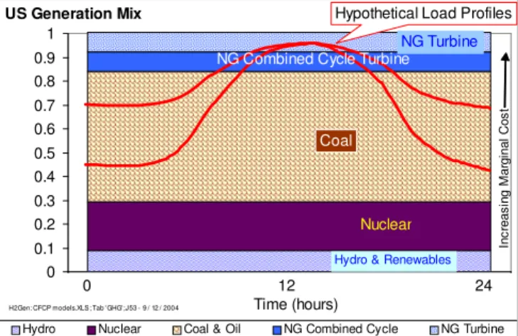
This marginal grid mix effect is illustrated in Figure 8, showing a hypothetical US utility grid over a 24-hour period. The electrical generators are layered in order of increasing marginal operating costs. Hydro and renewables have the lowest operating cost, and are therefore run as baseload8, followed by nuclear, then coal, and finally the natural gas generators that are used for peaking.

The red lines represent possible utility load profiles over 24 hours. Adding any new load will require this utility to increase the output from coal-based generators at night, and from natural gas generators during the peak day-time period. If vehicles

are charged from the grid, greenhouse gases will increase based primarily on coal plants, particularly if the vehicles are charged at night.

To simulate vehicle charging, the model calculates the fraction of grid generators that will have to be turned on using a PHEV charging profile (Figure 9) developed by the Electric Power Research Institute [11]. Most (74%) PHEV charging is off-peak at night in the EPRI model. The resulting estimates of the current marginal grid mix compared to the average grid

8 _{If water can be held behind dams without adversely affecting river flow or fisheries, then hydroelectricity can} be used for peak shaving, which maximizes its value.

0 0.1 0.2 0.3 0.4 0.5 0.6 0.7 0.8 0.9 1 1

Hydro Nuclear Coal & Oil NG Combined Cycle NG Turbine

0 12 24

Time (hours)

Hypothetical Load Profiles

Nuclear Hydro & Renewables Coal

NG Combined Cycle Turbine NG Turbine In c re a s in g M a rg in a l C o s t

H2Gen: CFCP models.XLS; Tab ' GHG';J53 - 9 / 12 / 2004

US Generation Mix

Figure 8. Illustration of marginal grid loads for a typical US electric utility 0% 2% 4% 6% 8% 10% 12% 1 2 3 4 5 6 7 8 9 10 11 12 13 14 15 16 17 18 19 20 21 22 23 24

Plug-In Hybrid Hourly Charging Percentage

Figure 9. PHEV charging profile suggested by EPRI

Renewables

& Nuclear Coal NG CC NG GT US Average 30.4% 50.1% 8.6% 10.9% US Marginal 0.0% 80.3% 3.9% 15.8% Cal. Average 39.0% 34.4% 11.7% 14.7% Cal. Marginal 0.0% 61.7% 21.5% 16.8% GHG.XLS, Tab 'Marginal Grid'; Q146;3/11/2008

mixes for the US and California are summarized in Table 5. In both cases, there is no credit for renewables and nuclear, the

two zero GHG sources. Our program estimates that 61.7% of electricity to charge vehicles in California will come from coal. For comparison, Mark Delucchi of UC-Davis estimates that 51.7% of electricity for charging car batteries in the West would come from coal and 15.2% from oil, or total of 66.9% high GHG emitting electricity [12].

For the near-term (2010) time period, we assumed current sources for the fuels: ethanol from corn, electricity from the grid, and hydrogen from natural gas.

7.

Key Dynamic

Assumptions

The methods of producing hydrogen, ethanol and electricity are expected to change over time, particularly if greenhouse gas reduction becomes a major priority. Transportation and electricity currently account for over 73% of all US GHG pollution (Figure 10). Reducing GHGs by 60% to 80% below 1990 levels by 2050 will require significant reductions in coal use for electricity (or carbon capture and storage-CCS) and reductions in petroleum use for transportation.

Electric Grid Mix. To simulate possible electrical grids of the future with a strong commitment to curbing GHGs, we averaged two projections

to 2030 by the EPA [13] and the DOE’s Energy Information Administration (EIA) to implement the GHG reduction goals of Senate Bill S.280 [14]. To provide the best benefit to battery EVs and plug-in hybrids, we also started with the current West Coast grid mix as represented by the Western Electricity Coordinating Council conglomerate of eleven western states. The electrical generators in these western states have a higher percentage of

-500 1,000 1,500 2,000 2,500 3,000 Res iden tial Com mer cial Indu stria l Tran spor tatio n Elec tric ity Coal Petroleum Natural Gas Greenhouse Gas Pollution

(Million Metric Tonnes of CO2/year)

40% 33.2%

16.9%

3.9% 6.1%

GHG emissions since 1949 EIA.XLS, Tab 'All,ElecPrw'; G99;3/11/2008

Figure 10. Current (2005) contributions to US greenhouse gas emissions from various sectors (all electricity was removed from residential, commercial and industrial sectors for this graphic)

Figure 11. Electrical grid production sources projected to 2100 based on EPA and EIA projections to 2030, scaled from WECC with significant carbon constraints; extra consumption shown for plug-in hybrids

-1,000 2,000 3,000 4,000 5,000 6,000 7,000 8,000 9,000 2005 2015 2025 2035 2045 2055 2065 2075 2085 2095

California/WECC Electricity Consumption Scaled to US

(Billion kWh/year) Renewables Nuclear Coal Coal with CCS Natural Gas

H2 Story: GHG.XLS, Tab 'Climat e Change Project ions'; U422;4/20/2008

Carbon Constrained Case

NG CC

Added Capacity for Gasoline Plug-in Hybrids

hydroelectricity and less coal-generated power than the rest of the nation. We then applied the average of the EPA and EIA

projections for the grid mix to the year 2030, and then extrapolated out to the year 2100, phasing in increasing fractions of renewables and also sequestration of carbon at integrated gasification combined cycle (IGCC) coal plants. This grid production mixture (Figure 11) was then used to estimate the marginal grid mix over time for the purpose of charging car batteries, applied to all sections of the US9.

The impact of these electrical generation changes on GHG pollution is shown in Figure 12, all relative to the 1990 US grid GHG’s. With the EIA’s 2008 Annual Energy Outlook projection to 2030, and a decrease in

the rate of electricity growth from 2030 to 2100 (excluding PHEV grid demand), the US utility GHGs would rise to 2.5 times the 1990 levels (150% increase) by 2100. With PHEVs, GHGs would rise to 200% above 1990 levels. With the assumptions used here, starting with the WECC grid mix (immediate drop

in 2005-2010), the grid GHGs would fall to 60% of 1990 levels by 2070 and to 75% below 1990 levels by 2090. With the low-carbon grid, adding PHEVs would have marginal impact. Even with this aggressive introduction of low-carbon generators, the GHGs from the grid would fall to only 20% below 1990 levels by 2050.

Electric Grid Capital Costs. We estimated the gross cost of installing these new low-carbon electrical generators using the capital expenditure costs and capacity factors for new generator technologies from the Electric Power Research Institute [15]. As

9 _{The extra electricity to charge PHEVs is assumed to come from the same mixture of generators as shown} without the PHEV consumption; extra grid capacity is needed with the EPRI charging schedule for PHEVs to accommodate 26% new on-peak demand; up to 700 billion kWh/year of existing off-peak power is assumed to be available from the grid for charging PHEVs at night

Figure 12. Estimated percentage change of grid greenhouse gas emissions relative to the 1990 US level assuming business as usual EIA projections through 2030, compared with the assumptions used here based on the WECC grid mix and significant carbon constraints over the century

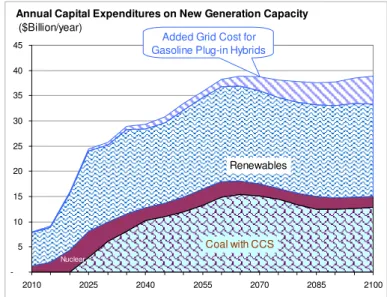
Figure 13. Estimated capital costs per year to install the new, low-carbon generators postulated in this model; also shown is the added cost to support plug-in hybrids

-5 10 15 20 25 30 35 40 45 2010 2025 2040 2055 2070 2085 2100

Annual Capital Expenditures on New Generation Capacity

($Billion/year)

Coal with CCS

Renewables

Added Grid Cost for Gasoline Plug-in Hybrids

Nuclear

GHG.XLS, Tab 'Climate Change Projections'; K421;3/24/2008

-100% -50% 0% 50% 100% 150% 200% 1980 1990 2000 2010 2020 2030 2040 2050 2060 2070 2080 2090 2100

% of Utility GHG above 1990 Levels

Business-as-usual; Extension of AEO 2008

US Projection based on California (WECC) Grid with Carbon Constraints

Business-as-usual; with PHEVs

shown in Figure 13, the electric utility industry would have to spend up to $30 billion per year by 2030 to install the new generators postulated for this assessment. This does not include any cost for new transmission and distribution equipment, but does include generator replacement after 30 years, assuming 20% salvage value. Note that we have assumed rather stringent energy conservation (Figure 11) in this model, with the rate of electricity consumption growth falling significantly after

2030 (without the added PHEV demand for electricity). If these energy conservation efforts fail to achieve these reductions, cost for new generator capacity would rise proportionately.

Hydrogen Sources. We have also assumed that the sources for hydrogen become greener over time. Hydrogen is made from natural gas initially as the least costly option for producing vehicle fuel, which immediately cuts GHGs by approximately 50% for FCVs compared to burning gasoline in a regular car. Further reductions in the hydrogen carbon footprint will be required, however, to meet the goals of a 60% to 80% reduction below 1990 levels.

The first move toward greener hydrogen postulated here is reforming ethanol at the fueling station. We assume that ethanol is made from corn initially, transitioning to cellulose and hemi-cellulose, starting with corn stover…the corn stalk and root residue that is currently left on the field. As fuel cell vehicles increase demand for hydrogen, we assume that hydrogen is made from biomass and natural gas and from coal gasification with carbon capture and storage (CCS). Finally, we assume that the bulk of the hydrogen is eventually made by electrolysis using green electricity from renewables or nuclear power, and from biomass gasification as shown in Figure 14.

Plug-in Hybrid Performance. The urban air and GHG pollution and petroleum consumption of PHEVs will depend on both their all-electric range (AER) and the percentage of energy drawn from the electrical grid. The AER is determined by the energy storage capacity of the PHEV’s battery bank. The larger the AER, the longer the vehicle can travel on grid electricity alone and the less frequently the vehicle will need to turn on its on-board power source. Figure 15 shows

Figure 14. Postulated sources of hydrogen over time

Story Simultaneous.XLS; Tab 'Graphs'; L 63 3/16 /2008

0 10 20 30 40 50 60 2000 2020 2040 2060 2080 2100 2120 0% 10% 20% 30% 40% 50% 60% 70%

PHEV All-Electric Range (Miles)

% Energy from Grid Percent of Energy from

the Electric Grid

All-Electric Range

Figure 15. The all-electric range and percentage of energy drawn from the electrical grid for plug-in hybrids

Hydrogen Production Sources

0% 10% 20% 30% 40% 50% 60% 70% 80% 90% 100% 2010 2020 2030 2040 2050 2060 2070 2080 2090 2100 Central Electrolysis (Renewable & Nuclear)

NG at Fueling Station

Coal IGCC + CCS

Ethanol at Fueling Station

Natural Gas SMR + CCS

Biomass Gasification

the AER and the corresponding fraction of PHEV energy drawn from the grid used in this model. The AER varies linearly from 12 to 52 miles, while the fraction of energy from the grid varies from 18% to 65% over the century. These data were derived from a report on PHEVs by the Electric Power Research Institute and the Natural Resources Defense Council where they estimated the fraction of grid energy for PHEVs with 10, 20 and 40 mile AER as a function of the annual vehicle miles traveled [16]. We extrapolated out to 52 miles range based on their data, using the vehicle miles traveled in this model.

8.

Key Static Transportation Results

Total Societal Cost. We have devised a single figure-of-merit to compare all vehicle/fuel combinations: the total societal costs including the costs of urban air pollution, greenhouse gas pollution, and the cost of oil imports. To account for GHG pollution, the model assumes a cost of $25/metric tonne of CO2 in 2010, rising linearly to $50/tonne by 2100. The model

assumes a societal cost of $60/barrel10 for oil to account for balance of trade and other macroeconomic costs and the military costs of protecting our oil supplies. This societal cost figure-of-merit changes over time as the relative “greenness” of fuel sources and the costs of GHGs vary. This figure-of-merit does not include any market acceptability information, but compares each vehicle on a one-for-one basis.

To further consolidate the data, we calculated the societal cost reduction factor for each

alternative vehicle/fuel combination; the reduction factor is the total societal cost of the baseline gasoline ICEV averaged over each time period divided by the societal cost of the alternative vehicle over that period. Thus if a gasoline ICEV generated $1,000 per year societal costs and a FCV produced $100 per year costs, then the FCV would have a 10 to one cost reduction factor. These cost reduction factors are summarized for the key vehicle/fuel combinations11 in Figure 7 above for the near-term (now to 2020), the mid-term (2021 to 2050) and the far-term (2051 to 2100.) These cost reduction factors are all based on the carbon constraints placed on the grid starting with the relatively clean West Coast (WECC) grid as described above.

As shown in Figure 7, the hydrogen-powered FCV reduces the total societal costs per car more than any other vehicle/fuel combination in all time periods. The FCV cuts societal costs by an average of 7.8 to one in the near-term compared to gasoline cars, rising to 20.4 to one in the far-term. The relative advantage of the FCV over the PHEVs would be even greater for the US electrical grid instead of the WECC grid mix assumed in this model.

The hydrogen-powered ICE plug-in hybrid is second-best, cutting societal costs by a factor of 5 initially, growing to 13.2 in the far-term.

10 _{This is not the price paid for oil, but an estimate of the additional societal cost in terms of economic loss} through trade imbalance, the cost of defending our oil supply, etc.

11 _{To reduce the data presented, we show only the best options in a given category. Thus the ethanol PHEV is} superior to either the ethanol ICEV or the ethanol HEV, so we do not show the latter two. Similarly, the FC HEV is superior to FC PHEV, while the hydrogen ICE PHEV is better than the hydrogen ICE HEV (although the H2 ICE HEV is superior for the dynamic simulations, since it does not have the limitation of access to night-time charging outlets). The diesel PHEV is similar to the gasoline PHEV, slightly better in some attributes and slightly worse in others, so we did not show the diesel PHEV.

The battery electric vehicle (BEV) is third-best, cutting societal costs between 4 to 10.6 to one over time. We have assumed here that the BEV uses advanced lithium-ion batteries that have achieved the DOE specific energy goal of 150 Wh/kg, which is a 50% improvement over the best Li-Ion energy battery developed to date[17]12. For widespread consumer acceptance, these BEVs would also have to reduce the long charging times to qualify for long-distance travel.

The fourth-best option is the ethanol-powered plug-in hybrid (PHEV). While ethanol supply will be limited, less would be needed for a PHEV than an ICEV.

The fifth-best option is the gasoline plug-in hybrid. Note that the average cost reduction factor for the gasoline PHEV, even in the long-term, is only 2.9 to one, compared to 20.4 to one for the FCV.

Finally, the gasoline (non-plug-in) hybrid offers the least advantage on a per-vehicle basis. The gasoline HEV essentially can only improve costs by the increased fuel economy compared to a conventional car,

assumed to be 1.39 to one in this model.

We now consider each of the three vehicle criteria separately:

Greenhouse Gas Pollution. The reduction factors for greenhouse gases (defined as the ratio of ICEV GHGs to the alternative vehicle GHGs) are shown in Figure 16. The data are similar to the societal cost reduction factors, but the ethanol PHEV has jumped to thrid place. Once again the hydrogen-powered FCV is superior for all time periods, cutting GHGs by factors of 2 to 11 compared to the

gasoline ICEV. The BEV actually has higher GHG emissions than a gasoline car in the near-term, before the electrical grid carbon constraints take effect, so the reduction factor is slightly less than one in the near-term.

Urban Air Pollution. The static urban air pollution reduction factors are shown in Figure 17, with the FCV superior to all the others. Surprisingly, the BEV has lower air pollution reduction factors (more pollution) than the ethanol PHEVs and gasoline PHEVs in the near-term. One normally thinks of the BEV as a zero emission vehicle. However, the Argonne GREET model calculates substantial urban air pollution from BEVs. Much of this pollution

12 _{Although a 2008 DOE energy storage R&D progress report [18] listed 100 wh/kg as the goal for PHEV} batteries, in which case the 150 Wh/kg assumed here would be 50% above the DOE goal.

Figure 16. Greenhouse gas reduction factors compared to gasoline ICEVs -2 4 6 8 10 12 FCV H2 ICE PHEV EtOH PHEV BPEV Gasoline PHEV Gasoline HEV Near-Term Mid-Term Far-Term Greenhouse Gas Reduction Factors per Vehicle

is due to SOx and NOx from electrical power plants either in or up wind of the urban airshed. Some particulates are also generated by the tires and brakes of a BEV.

Oil Consumption. The oil consumption reduction factors are huge for the FCV, hydrogen ICE PHEV and the BPEV, since they use virtually no oil (nearly division by zero!) We put them off-scale in Figure 18 to show the relative comparison of the ethanol and gasoline PHEVs and the gasoline HEVs. Significant petroleum is used to grow corn or other biomass, to transport the biomass and ethanol, etc., so the ethanol oil reduction factors are limited to the range between 6 and 12 to one.

9.

Dynamic Transportation

Simulation Assumptions

The static per vehicle data in Section 8 above do not take into account the marketability of the various alternative vehicle/fuel combinations or the availability of alternative fuels. The gasoline HEVs and ethanol (E-85) ICEVs are already on the road in limited numbers. Others such as PHEVs and FCVs will require further technical development and cost reductions before they satisfy a large segment of consumers. Battery EVs may

take even longer to overcome the limited range/refueling time dilemma. To account for these differences in technical/ economic readiness, we have simulated the gradual introduction of advanced vehicles into the fleet according to the modified logistic market share curves shown in Figure 19.

We have analyzed four different main vehicle/fuel scenarios:

• Base Case gasoline HEV Scenario • Ethanol PHEV Scenario

• Gasoline PHEV Scenario • Hydrogen FCV Scenario

Figure 17. Urban air pollution reduction factors relative to gasoline ICEVs

Figure 18. Oil consumption reduction factors -2 4 6 8 10 12 14 16 18 20 FCV H2 ICE PHEV BPEV EtOH PHEV Gasoline PHEV Gasoline HEV Near-Term Mid-Term Far-Term

Oil Reduction Factors per Vehicle

(Relative to gasoline ICEV) -0.5 1.0 1.5 2.0 2.5 3.0 3.5 4.0 4.5 5.0 FCV BPEV H2 ICE PHEV EtOH PHEV Gasoline PHEV Gasoline HEV Near-Term Mid-Term Far-Term Urban Air Reduction Factors per Vehicle (Relative to gasoline ICEV)

In addition we analyzed a gasoline ICEV-only case, excluding all hybrids, the BEV and H2 ICE HEV cases. The mix of new car sales for each scenario is illustrated in Figures 20 through 23.

For the base case, we assume that gasoline hybrids continue their current ramp-rate in sales, reaching 50% market share by 2024, with the remainder of all cars sold conventional gasoline ICEVs (Figure 20).

For the gasoline PHEV scenario,

we assume that the plug-in hybrids have a sales curve delayed by six years, or 50% sales share by 2032. We assume that 75% of all vehicles have access to night-time power outlets13. Gasoline HEVs continue to be sold as shown in Figure 21. Ethanol PHEVs enter the marketplace with the same basic sales share potential as gasoline PHEVs, but with the added constraint of limited ethanol production capacity. Ethanol consumption ramps up to 14 billion gallons by 2022 (limited by

13 _{EIA and Census Bureau data estimate that 45% to 50% of car owners have garages or carports (some of which} may actually still have cars inside!); assume that another 25% have driveways or assigned off-street parking places that could accommodate an outdoor charging port.

H2 Energy Story.XLS; Tab 'Annual Sales';HI 155 3/11 /2008

H2 Energy Story.XLS; Tab 'Annual Sales';IK 182 3/11 /2008 0% 10% 20% 30% 40% 50% 60% 70% 80% 90% 100% 2000 2010 2020 2030 2040 2050 2060 2070 2080 2090 2100 Market Share of New Car Sales

Gasoline HEVs, & EtOH ICEVs & HEVs

H2 ICE HEVs & PHEVs

H2 FC HEVs, FC PHEVs & BPEVs

Diesel HEVs, Gasoline, Deisel &EtOH PHEVs

Figure 19. Percentage market share of new vehicles sold in the US for each of the alternative vehicles

Percentage of New Car Sales

0% 10% 20% 30% 40% 50% 60% 70% 80% 90% 100% 2005 2015 2025 2035 2045 2055 2065 2075 2085 2095 Gasoline ICEVs Gasoline HEVs

Figure 20. Annual market share of gasoline ICEVs and gasoline HEVs for the base case scenario

Figure 21. Market share of new cars sold for the gasoline plug-in hybrid scenario

Figure 22 Market share of new cars sold for the ethanol plug-in hybrid scenario

Percentage of New Car Sales

0% 10% 20% 30% 40% 50% 60% 70% 80% 90% 100% 2005 2015 2025 2035 2045 2055 2065 2075 2085 2095 Gasoline ICEVs Gasoline PHEV Gasoline HEV

Percentage of New Car Sales

0% 10% 20% 30% 40% 50% 60% 70% 80% 90% 100% 2005 2015 2025 2035 2045 2055 2065 2075 2085 2095 Gasoline

ICEVs Gasoline HEV

PHEV sales), less than the 36 billion gallons/year Congressional goal, and continues up to a level of 120 billion gallons per year, by 2060. NRDC suggested that up to 120 billion gallons/year of cellulosic ethanol could be produced in the US, equivalent to 7.9 million barrels/day of gasoline on an energy basis [19]. The fuel cell vehicle scenario assumes that FCVs are sold into the existing gasoline HEV/PHEV and ethanol PHEV markets. The FCV market penetration curve is also delayed relative to the gasoline PHEV market curve, such that FCVs have the potential of reaching 50% of all new cars sold by 2035, with market

share increasing over time as shown in Figure 23. Both the H2 ICE HEV and the BEV scenarios follow the sales projection of Figure 23, replacing the FC HEV sales fractions.

10.

Hydrogen Infrastructure Costs

The U.S. Department of Energy and its contractors have developed the H2A hydrogen infrastructure cost estimating model. This model predicts that the cost of providing hydrogen will be minimized initially by installing steam methane reformers at fueling stations to convert natural gas and water to hydrogen. This avoids the necessity of installing a costly hydrogen pipeline system that would be severely under-utilized when there are very few hydrogen vehicles on the road. Hydrogen fueling stations are added when and where they are needed to match the introduction of hydrogen vehicles in each region of the country.

For purposes of estimating GHGs and urban pollution, we have assumed that hydrogen production shifts gradually from on-site distributed generation to central production with either truck or pipeline delivery. For costing purposes, however, it is easier to estimate costs for on-site production only and avoid the complexity of deciding when and where to begin building large central hydrogen production plants and hydrogen pipeline distribution systems. We assume that the shift to central production will occur when there are enough FCVs in a given region to make central production and hydrogen delivery by either truck or pipeline less costly than on-site distributed generation. Hence the costs calculated here should be considered an upper bound on the hydrogen fueling supply system.

The fueling equipment has an expected life of 20 years. At the end of its useful life, all equipment is replaced with zero assumed salvage value (another conservative assumption.) By the last quarter of the century, the annual costs reach $38 billion per year including both expansions of the hydrogen infrastructure as well as replacement of older fueling systems. This is approximately the same as the cost of converting the electrical grid to low-carbon sources, especially if extra grid capacity must be installed to support plug-in hybrids (See Figure 13).

Figure 23. Market share of new vehicles sold for the fuel cell vehicle scenario

Percentage of New Car Sales

0% 10% 20% 30% 40% 50% 60% 70% 80% 90% 100% 2005 2015 2025 2035 2045 2055 2065 2075 2085 2095 Gasoline

ICEVs Ethanol PHEVs

Gasoline PHEV Fuel Cell

Fueling Station Capacity Factor. As shown in Figure 24, the capacity factor approaches 70% by 2018 in this model after a cumulative hydrogen infrastructure investment of $9 billion for

6,500 hydrogen stations. At this point, the energy companies will start making the 10% real, after-tax return on the capital investments that is assumed in the model to calculate the price of hydrogen to drivers. In other words, little or no additional government incentives would be required to continue building the hydrogen infrastructure after the 2018 time period.

Hydrogen vs. Gasoline Infrastructure Costs. To put the hydrogen infrastructure expenditures in perspective, Figure 4 (shown above)

compares the hydrogen infrastructure cost with the recent history of actual energy company capital investments in the US gasoline and diesel fuel infrastructure. In 2008, the Oil and Gas Journal estimates that the energy companies will spend almost $200 billion in the US on capital items [20]. Some of these expenditures are for natural gas and some for non-fuel uses of crude oil. We have not located a source for the fraction of these capital expenditures that should be attributed to gasoline and diesel fuel, so we estimated that fraction as follows. The energy companies produced more natural gas (19 quads) in the US than oil (13.2 quads). However, the production of gasoline from crude oil

is much more capital intensive than the production of line natural gas from well-head gas. One measure of this cost is the price charged for these two products. In 2006, natural gas prices averaged $6.24/MBTU, while gasoline averaged $21.06/MBTU, including highway taxes. Subtracting 48 cents/gallon ($3.84/MBTU) average highway taxes, gasoline cost $17.22/MBTU. If we apply these costs times the production of oil and gas, the net revenues from natural gas were $119 billion and $227 billion for oil turned into gasoline.

By this revenue measure, natural gas accounted for 34% of the total capital expenditures, so we can associate 66% of the $200 billion spent in 2008 to petroleum, or $132 billion. Gasoline and diesel fuel account for approximately 67% of the output from US oil refineries[21], so the final estimate of their share of capital expenditures for 2008 is $87

Figure 24. Number of hydrogen fueling stations, the cumulative _{capital costs for those stations, and the average} capacity factors in the early years of FCV deployment

Table 6. Costs for distributed hydrogen fueling systems

Single Qty 500 Qty 100 kg/day $ 772,800 $ 535,000 500 kg/day $ 2,212,000 $ 1,534,000 1,500 kg/day $ 4,181,700 $ 2,900,000 H2 Energy Story.XLS; Tab 'Annual Sales';EC 18 3/22 /2008

Fueling Station Costs Capacity

H2 Energy Story.XLS; Tab 'Annual Sales';DB 24 4/20 /2008

-1,000 2,000 3,000 4,000 5,000 6,000 7,000 8,000 9,000 2006 2008 2010 2012 2014 2016 2018 0% 10% 20% 30% 40% 50% 60% 70% 80% 90% 100%

Cumulative Hydrogen Infrastructure Capital Expenditures

(US$ millions)

& # of H2 Fueling Stations

Average Capacity Factor Cumulative Capex Capacity Factor # of H2 Stations

billion as shown in Figure 4. Thus 2008 capital expenditures for gasoline & diesel infrastructure far exceed the expected 2030 costs for the hydrogen infrastructure.

11.

Natural Gas Resources

Some observers have suggested that by replacing gasoline with hydrogen made from natural gas we would just be switching from one foreign fossil fuel dependency to another. Several relevant points on natural gas usage for hydrogen production include:

• Natural gas would be a temporary transition energy source for hydrogen until lower

carbon sources such as biofuels, electrolysis of water using renewables, biofuels, nuclear or coal with sequestration become practical and affordable.

• US natural gas consumption would increase temporarily by less than 12% to supply

hydrogen for fuel cell vehicles in this scenario, falling thereafter as hydrogen is made from other sources

• Every BTU of natural gas used to make hydrogen for a FCV displaces approximately

two BTUs of crude oil, so hydrogen from natural gas would cut total fossil fuel use by a factor of two14

• The world has slightly more natural gas resources than crude oil resources, and the

world is consuming oil faster than natural gas. Therefore cutting some petroleum use and increasing natural gas consumption by a lesser amount actually helps to correct the imbalance developing between global oil and gas resources.

• The Middle East holds 55% of oil resources but only 31% of natural gas resources, so

slightly shifting from oil to gas at least diminishes dependence on fossil fuels from this unstable region.

If we assume constant natural gas consumption after 2030 based on the AEO2008 projections, then the addition of fuel cell vehicles according to the scenarios reported here would temporarily increase US natural gas consumption by less than 12% (right-hand scale of Figure 25) in the 2060 time period, then falling rapidly thereafter.

14 _{Crude oil BTU consumption / natural gas BTU consumption = 2.45 x .75/.86 = 2.1, assuming FCV fuel} economy is 2.45 times that of ICEVs, SMR efficiency =75% and gasoline refinery efficiency = 86%.

Figure 25. Comparison of projected US natural gas consumption assuming a flat rate after 2030 and the natural gas needed to make hydrogen in the FCV scenario, which is less than 12% of US consumption.

H2 Energy Story.XLS; Tab 'NG 2008'; U 76 3/21 /2008

0 5 10 15 20 25 30 2000 2020 2040 2060 2080 2100 0.0% 2.0% 4.0% 6.0% 8.0% 10.0% 12.0% 14.0% Natural Gas Consumption

(Quads) H2 NG % AEO 2008 NG Projections Natural Gas to Make Hydrogen % NG to Make Hydrogen

Natural gas vs. crude oil resources. The global natural gas resources (proved reserves, reserve growth, and undiscovered natural gas) are slightly larger than the crude oil resources. The curves in Figure 26 assume that

no new oil or gas is found, and the world consumption of both fuels continues at current rates. The two extra curves assume that 50% of all the world’s cars sold are FCVs by 2050 (rising to 100% by 2100) and all hydrogen is made from natural gas.

Under these conditions, the world’s supply of oil and gas would follow the trajectories shown in Figure 26. Without any new discoveries, the world would run out of petroleum before 2050. By adding FCVs, we would save approximately 900 quads of oil by 2050, adding a few years more global consumption. Natural gas reserves would decrease by approximately 470 quads under these worst-case conditions.

We conclude that even if all FCVs use hydrogen from natural gas, the impact on natural gas resources would be minimal on a global scale, and the slight decrease in natural gas consumption is more than offset by the larger increase in oil resources. The net effect is to partially improve the balance between natural gas and oil consumption while cutting total fossil fuel use in half.

Acknowledgments

We would like to thank the many people who have contributed over the years to the development and review of these vehicle simulation models, beginning with Ira Kuhn, Brian James, Julie Perez and their colleagues at Directed Technologies, Inc.; Ron Sims, Brad Bates, Mujeeb Ijaz and colleagues (then at the Ford Motor Company); Bob Shaw (Arête), Barney Rush (CEO) and Frank Lomax (CTO) and all our co-workers at H2Gen; the many players at

the Department of Energy including, among others, Sig Gronich, Neil Rossmeissl, Steve Chalk, JoAnn Milliken, Mark Paster and Arlene Anderson; Joan Ogden and Mark Delucchi and their colleagues at the University of California at Davis; Michael Wang and colleagues at the Argonne National Laboratory; Bob Rose at the US Fuel Cell Council and, more recently, to the members of the National Hydrogen Association task force developing a new hydrogen energy story, headed by Frank Novachek of Xcel Energy.

H2 Energy Story.XLS; Tab 'NG-Oil Resources';BA141 - 2 / 28 / 2008 -4,000 -2,000 0 2,000 4,000 6,000 8,000 10,000 12,000 14,000 2000 2010 2020 2030 2040 2050 NG Baseline NG + Optimistic FCVs Oil + Optimistic FCVs Oil Baseline FCVs Decrease Natural Gas Resources 470 Quads FCVs Increase Crude Oil Resources by 900 Quads

Remaining Global Resources

(Quads)

Figure 26. Hypothetical illustration of the impact of 50% FCV global sales by 2050, showing that world’s crude oil resources would increase much more than natural gas resources would decrease, tending to right the imbalance that would otherwise occur

References

1. Michael Q. Wang : Greenhouse gases, Regulated Emissions, and Energy use in Transportation, Argonne

National Laboratory, http://www.transportation.anl.gov/software/GREET/ ; Argonne has also released version 2.8a that includes the impact of vehicle manufacturing.

2. The DOE H2A model currently covers hydrogen production and delivery options, with others in process

http://www.hydrogen.energy.gov/h2a_analysis.html

3. The Hydrogen Economy: Opportunities, Costs, Barriers, and R&D Needs, the National Research Council

and the National Academy of Engineering, 2004, http://www.nap.edu/catalog/10922.html

4. Norman Brinkman (GM), Michael Wang (ANL) et al., Well-to-Wheels Analysis of Advanced Fuel/Vehicle Systems—A North American Study of Energy Use, Greenhouse Gas Emissions, and Criteria Pollutant Emissions, May 2005

5. M.A. Kromer and J. B. Heywood (MIT), “A comparative assessment of electric propulsion systems in the 2030 US light-duty vehicle fleet,” SAE Technical Paper Series 2008-01-0459, April 2008.

6. Mark A. Delucchi, Summary of the nonmonetary externalities of motor-vehicle use; Report #9: The Annualized Social Cost of Motor-Vehicle Use in the United States, based on 1990-1991 Data, University of

California at Davis, UCD-ITS-RR-96-3 (9) rev.1, September 1998, Revised October 2004.

7. Todd A Litman, Transportation Cost Analysis: Techniques, Estimates and Implications, Victoria Transport

Policy Institute, June 2002. www.vtpio.org

8. AEA Technology Environment, Damages Per Tonne Emission of PM2.5, NH3, SO2, Nox and VOCs from each EU25 Member State, Clean Air for Europe (CAFÉ) Programme, European Commission, 2005

http://ec.europa.eu/environment/air/café/activities/cba.htm

9. Mike Holland and Paul Watkins, Estimates of Marginal External Costs of Air Pollution in Europe,

European Commission, 2002 http://europa.eu.int/comm/environment/enveco/studies2.htm

10. M.Q. Wang, D.J. Santini, and S. A. Warinner, Methods of Valuing Air Pollution and Estimated Monetary Values of Air Pollutants in Various US Regions, Argonne National Lab, 1994, and M.Q. Wang, D.J. Santini,

and S. A. Warinner, Monetary Values of Air Pollutants in Various US Regions, Transportation Research

Record, 1475, pp. 33-41,1995.

11. Environmental Assessment of Plug-In Hybrid Electric Vehicles; Volume 1: Nationwide Greenhouse Gas Emissions, by the Electric Power Research Institute and the Natural Resources Defense Council, Final

Report 1015325, July 2007.

12. Mark A. Delucchi, A lifecycle emissions model (LEM): lifecycle emissions from transportation fuels, motor vehicles, transportation modes, electricity use, heating and cooking fuels, and materials, Institute for

Transportation Studies, University of California, Davis, Report # UCD-ITS-RR-03-17, December 2003, Table 15, pg. 330

13. EPA Analysis of the Climate Stewardship and Innovation Act of 2007, S.280, July 16, 2007, U.S. Environmental Protection Agency, Office of Atmospheric Programs, contact: Francisco de la Chesnaye,

www.epa.gov/climatechange/economicanalyses.html

14. Energy Information Administration, “Energy Market and Economic Impacts of S.280, the Climate Stewardship and Innovation Act of 2007,” EIA Report # SR/OIAF/2007-04, July 2007.

15. Electric Power Research Institute, “The Power to Reduce CO2 Emissions: The Full Portfolio,” by the EPRI Energy Technology Assessment Center, Discussion Paper, August 2007.

16. Environmental Assessment of Plug-In Hybrid Electric Vehicles; Volume 1: Nationwide Greenhouse Gas Emissions, by the Electric Power Research Institute and the Natural Resources Defense Council, Final

Report 1015325, Figure 2-3, page 2-14, July 2007

17. Edward J. Wall, Program Manager, FreedomCAR and Vehicle Technologies, Plug-In Hybrid Electric Vehicle R&D Plan, U. S. Department of Energy, February 2007, pg.18

18. David Howell, Manager, Energy Storage R&D, FY2007 Progress Report for Energy Storage Research and Development, U.S. Department of Energy, January 2008, pg. 7

19. Nathanael Greene, Growing Energy: How Biofuels Can Help End America’s Oil Dependence, Natural

Resources Defense Council, December 2004.

20. Marilyn Radler, “Oil and gas capital spending to rise in US, fall in Canada,” Oil & Gas Journal, Volume

105, Issue 13, Apr 02, 2007 & “Capital budgets grow in US, drop in Canada,” April 28,2008, p.20 21. Stacy C. Davis and Susan W. Diegel, Transportation Energy Data Book, 26th Edition, Center for

Transportation Analysis, Oak Ridge National Laboratory #6978, US Department of Energy, 2007, Table 1.10