6.1 Introduction 113
Chapter 6
Comparing Two Proportions
6.1 IntroductionIn this chapter we consider inferential methods for comparing two population propor-tions p1 and p2. More specifically, we consider methods for making inferences about the
difference p1−p2 between two population proportions p1 andp2. The inferential methods
for a single proportion p discussed in Chapter 5 are based on a large sample size normal approximation to the sampling distribution of ˆp. The inferential methods we will discuss in this chapter are based on an analogous large sample size normal approximation to the sampling distribution of ˆp1−pˆ2. Sections 6.2 and 6.3 deal with inferential methods
appro-priate when the data consist of independent random samples. The modifications needed for dependent (paired) samples are discussed in Section 6.4.
6.2 Estimation for two proportions (independent samples)
In some applications there are two actual physical dichotomous populations so that p1 denotes the population success proportion for population one and p2 denotes the
pop-ulation success proportion for poppop-ulation two. In other applications, such as randomized comparative experiments p1 and p2 denote hypothetical population success probabilities
corresponding to two treatments. We will assume that the data correspond to two inde-pendent sequences of Bernoulli trials: a sequence of n1 Bernoulli trials with population
success probabilityp1 and an independent sequence of n2 Bernoulli trials with population
success probabilityp2. The assumption that these are independent sequences of Bernoulli
trials means that the outcomes of all n1+n2 trials are independent. When sampling from
physical populations these assumptions are equivalent to assuming that the data consist of two independent simple random samples (of sizesn1 andn2) selected with replacement
from dichotomous populations with population success proportionsp1 andp2. In this
con-text the assumption of independence basically means that the method used to select the random sample from the first population is not influenced by the method used to select the random sample from the second population, and vice versa.
The observed success proportions ˆp1 and ˆp2 are the obvious estimates of the two
pop-ulation success proportions p1 and p2; and the difference ˆp1−pˆ2 between these observed
success proportions is the obvious estimate of differencep1−p2 between the two population
success proportions. The behavior of ˆp1−pˆ2 as an estimator ofp1−p2 can be determined
from its sampling distribution. As you might expect, since ˆp1 and ˆp2 are unbiased
114 6.2 Estimation for two proportions (independent samples)
distribution of ˆp1−pˆ2 has mean equal top1−p2. The standard deviation of the sampling
distribution of ˆp1−pˆ2 is the population standard error of ˆp1−pˆ2
S.E.(ˆp1−pˆ2) = s p1(1−p1) n1 + p2(1−p2) n2 .
Notice that the population variance var(ˆp1−pˆ2) (the square of S.E.(ˆp1−pˆ2)) is equal to the
sum of the population variance of ˆp1 and the population variance of ˆp2. This property is a
consequence of our assumption that the random samples are independent. This expression for the standard error of the difference between two sample success proportions is not appropriate if the random samples are not independent.
As was the case for the sampling distribution of a single sample proportion, the sam-pling distribution of ˆp1−pˆ2 is not the same when ˆp1 and ˆp2 are based on samples selected
without replacement as it is when ˆp1 and ˆp2 are based on samples selected with
replace-ment. In both sampling situations, the mean of the sampling distribution of ˆp1 −pˆ2 is
p1−p2. Thus ˆp1−pˆ2 is an unbiased estimator of p1−p2, whether the samples are selected
with or without replacement. On the other hand, as with a single proportion, the standard error of ˆp1−pˆ2 is smaller when the samples are selected without replacement. This implies
that, strictly speaking, the confidence interval estimates of p1−p2 given below, which are
based on the assumption that the samples are selected with replacement, are not appro-priate when the samples are selected without replacement. However, if the sizes of the two populations are both very large relative to the sizes of the samples, then, for practical pur-poses, we can ignore the fact that the samples were selected without replacement. Hence, when we have samples selected without replacement and we know that the populations are very large, it is not unreasonable to compute a confidence interval estimate of p1−p2 as
if the samples were selected with replacement.
Remark. When pˆ1 and pˆ2 are computed from independent simple random samples of
sizes n1 and n2 selected without replacement from dichotomous populations of sizes N1
and N2, the population standard error of pˆ1−pˆ2
S.E.(ˆp1−pˆ2) = s f1 p1(1−p1) n1 +f2 p2(1−p2) n2 ,
is smaller than the population standard error for independent samples selected with re-placement. In this situation there are two finite population correction factors f1 =
(N1 − n1)/(N1 − 1) and f2 = (N2 − n2)/(N2 −1) and the effect on the standard
er-ror is most noticeable when one or both of the N′s is small relative to the corresponding
n. If N1 and N2 are both very large relative to the respective n1 and n2, then f1 ≈ 1,
6.2 Estimation for two proportions (independent samples) 115 We will consider inferential methods based on a large sample size normal approxima-tion to the sampling distribuapproxima-tion of ˆp1 −pˆ2. This normal approximation is analogous to
the normal approximation to the sampling distribution of ˆp of Section 5.2. In the present context the normal approximation simply says that, when both n1 and n2 are large, the
standardized value of ˆp1 −pˆ2, obtained by subtracting the population difference p1−p2
and dividing by the population standard error of ˆp1−pˆ2, behaves in approximate
accor-dance with the standard normal distribution. For completeness, a formal statement of this normal approximation is given below.
The normal approximation to the sampling distribution of pˆ1 −pˆ2. Let pˆ1
de-note the observed proportion of successes in a sequence of n1 Bernoulli trials with success
probability p1 (or equivalently the observed proportion of successes in a simple random
sample drawn with replacement from a dichotomous population with population success proportion p1). Let pˆ2 denote the observed proportion of successes in a sequence of n2
Bernoulli trials with success probabilityp2 (or equivalently the observed proportion of
suc-cesses in a simple random sample drawn with replacement from a dichotomous population with population success proportion p2). Assume that these two sequences of Bernoulli
trials (or random samples) are independent. Finally let a < b be two given constants and S.E.(ˆp1−pˆ2) = s p1(1−p1) n1 + p2(1−p2) n2 . If n1 and n2 are sufficiently large, then the probability that
(ˆp1−pˆ2)−(p1−p2)
S.E.(ˆp1−pˆ2)
is betweenaandbis approximately equal to the probability that a standard normal variable Z is between a andb. In symbols, using ≈to denote approximate equality, the conclusion from above is that, for sufficiently large values of n1 and n2,
P a ≤ (ˆp1−pˆ2)−(p1−p2) S.E.(ˆp1−pˆ2) ≤ b ≈P(a≤Z ≤b).
Remark. If the two populations being sampled are very large relative to the sizes of the samples, then, for practical purposes, this normal approximation to the sampling distribution of pˆ1 −pˆ2 may also be applied when pˆ1 and pˆ2 are based on independent
simple random samples selected without replacement.
The starting point for using this normal approximation to construct a 95% confidence interval estimate of the difference p1−p2 between the two population success proportions
is the approximate probability statement
P |(ˆp1−pˆ2)−(p1−p2)| ≤1.96S.E.(ˆp1−pˆ2)
116 6.2 Estimation for two proportions (independent samples)
This probability statement indicates that the probability that the actual difference p1−p2
is within 1.96S.E.(ˆp1−pˆ2) units of the observed difference ˆp1−pˆ2 is approximately .95. As
was the case with the analogous interval for one proportion, this interval is not computable, since it involves the population standard error S.E.(ˆp1−pˆ2) which depends on the unknown
parameters p1 and p2 and is therefore also unknown.
The method we used to derive the Wilson confidence interval for a single proportion will not work in the present context. Therefore, in the present context we will consider a confidence interval estimate of the difference p1 −p2 based on the estimated difference
ˆ
p1−pˆ2 and the estimated standard error of ˆp1−pˆ2
d S.E.(ˆp1−pˆ2) = s ˆ p1(1−pˆ1) n1 + pˆ2(1−pˆ2) n2 .
We will refer to this estimated standard error as the standard error for estimation. The margin of error of ˆp1 −pˆ2 is obtained by multiplying this estimated standard error
by a suitable constant k. (Recall that: for a 95% confidence level k = 1.96, for a 90% confidence level k = 1.645, and for a 99% confidence level k = 2.576.) The 95% margin of error of pˆ1−pˆ2 is
M.E.(ˆp1−pˆ2) = 1.96S.E.(ˆd p1−pˆ2)
and the interval from (ˆp1 −pˆ2)−M.E.(ˆp1 −pˆ2) to (ˆp1 −pˆ2) + M.E.(ˆp1 −pˆ2) is a 95%
confidence interval estimate of the difference p1−p2. Thus we can claim that we are 95%
confident that the differencep1−p2 between the population success proportions is between
(ˆp1−pˆ2)−M.E.(ˆp1−pˆ2) and (ˆp1−pˆ2) + M.E.(ˆp1−pˆ2).
Recall that it is the estimate ˆp1 −pˆ2 and the margin of error M.E.(ˆp1 −pˆ2) which vary
from sample to sample. Therefore, the 95% confidence level applies to the method used to generate the confidence interval estimate.
Example. Rural versus urban voter preferences. Suppose that a polling or-ganization has separate listings of all the registered voters in a large rural district and a large urban district and wishes to compare the proportions of voters in these districts who favor a proposition which is to appear on an upcoming election ballot. Let p1 denote
the proportion of all registered voters in the rural district who favor the proposition at the time of the poll and let p2 denote the proportion of all registered voters in the urban
district who favor the proposition at the time of the poll. (In terms of the box of balls analogy of Chapter 5, we now have two boxes of balls with p1 denoting the proportion of
6.2 Estimation for two proportions (independent samples) 117 The most obvious way to obtain independent random samples in this scenario is to: (1) randomly generate a set ofn1 labels for the rural district, contact the corresponding voters,
and compute the estimate ˆp1for the voters in the rural district; and, (2) randomly generate
a set ofn2 labels for the urban district, contact the corresponding voters, and compute the
estimate ˆp2 for the voters in the urban district. (Select a simple random sample of balls
from box one and compute ˆp1 and, independently, select a simple random sample of balls
from box two and compute ˆp2.) Assuming that simple random samples are selected (with
replacement or from large populations) this method clearly yields independent samples and the confidence interval method described above is valid.
Now suppose that we do not have separate listings of the rural voters and the urban voter but instead have a single listing of all registered voters in a large district which includes both rural and urban voters. In this situation we could randomly generate a set of nlabels for the entire district, contact the corresponding voters, and in addition to determining whether the voter favors the proposition also determine whether the voter lives in a rural or urban area. We could then partition the simple random sample ofnvoters into the subsample ofn1 voters who live in a rural area and the subsample ofn2 voters who live
in an urban area. (This is like labeling the balls in box one with a one, labeling the balls in box two with a two, then combining the balls in a single box, selecting a simple random sample ofnballs from this box, and dividing it to get a sample ofn1balls from box one and
a sample ofn2balls from box two.) This approach yields independent random samples but,
technically (based on the formal definition), these random samples are not simple random samples, since the sample sizes n1 and n2 were not selected in advance. Actually this is
not a problem, since it is readily verified that the samples can be viewed as independent sequences of Bernoulli trials (exactly if selection is with replacement and approximately if selection is without replacement from a large population and both subpopulations are also large). Therefore, the confidence interval method described above is also valid when this alternate method of forming independent random samples by partitioning a simple random sample is used.
Example. An opinion poll. The purpose of this example is to demonstrate the application of a 95% confidence interval for p1−p2. To make the numbers more realistic
we will use numbers from a New York Times/CBS News poll conducted September 9–13, 2005. To place this in context note that hurricane Katrina made landfall on September 1, 2005. Like all such national polls this poll was not based on a simple random sample; it employed a complex random sampling method involving stratification and clustering.
Suppose that a listing of telephone numbers for a well–defined population of adults in the U.S. was used to select a simple random sample ofn= 1,167 adults. When asked “Are you white, black, Asian, or some other race?” 877 of these 1,167 adults chose white and 211 chose black. Therefore, we have independent simple random samples of size n1 = 877
118 6.2 Estimation for two proportions (independent samples)
(from the subpopulation of white adults) and n2 = 211 (from the subpopulation of black
adults).
First consider the responses to question 10: “Do you think George W. Bush has the same priorities for the country as you have, or not?” Let p1 denote the proportion of
all white adults in this population who would respond “has the same priorities” and let p2 denote the proportion of all black adults in this population who would respond “has
the same priorities”. Of the n1 = 877 whites 360 responded “has the same priorities”
giving ˆp1 = .4105 while 27 of the n2 = 211 blacks responded “has the same priorities”
giving ˆp2 =.1280. These data clearly suggest that the population proportion p1 is greater
than the population proportion p2, since 41.05% of the whites responded “has the same
priorities” while only 12.80% of the blacks responded this way. In this situation we are 95% confident that p1−p2 is between .2269 and .3381. Since this entire interval is positive
we can conclude that we are 95% confident that the population proportion of whites who would have responded “has the same priorities” if all had been asked exceeds the analogous population proportion for blacks by at least .2269 and perhaps as much as .3381. In other words, we are 95% confident that the percentage of all whites who would have responded “has the same priorities” exceeds the corresponding proportion for blacks by between 22.69 and 33.81 percentage points.
Next consider the responses to question 14: “Do you think Congress has the same priorities for the country as you have, or not?” Let p1 denote the proportion of all white
adults in this population who would respond “has the same priorities” and let p2 denote
the proportion of all black adults in this population who would respond “has the same priorities”. Of the n1 = 877 whites 252 responded “has the same priorities” giving ˆp1 =
.2873 while 51 of then2 = 211 blacks responded “has the same priorities” giving ˆp2 =.2417.
In this case it is not clear whether the data suggest that the population proportion p1 is
greater than the population proportion p2, since the sample proportions are reasonably
similar. In this situation we are 95% confident that p1−p2 is between –.0194 and .1107.
Since the lower limit of this interval is negative (suggesting p1 < p2) and the upper limit
of this interval is positive (suggesting p1 > p2) we cannot exclude the possibility that the
population proportionsp1 andp2 are the same.
Finally consider the responses to question 62: “As a result of the recent increase in gas prices, have you cut back on household spending on other things?” Let p1 denote
the proportion of all white adults in this population who would respond yes and let p2
denote the proportion of all black adults in this population who would respond yes. Of the n1 = 877 whites 517 responded yes giving ˆp1 =.5895 while 158 of the n2 = 211 blacks
responded yes giving ˆp2 =.7588. These data clearly suggest that the population proportion
p1 is less than the population proportion p2, since only 58.95% of the whites responded
6.2 Estimation for two proportions (independent samples) 119 p1 −p2 is between -.2263 and -.0923 (or equivalently that p2 −p1 is between .0923 and
.2263). Since this entire interval (for p1−p2) is negative we can conclude that we are 95%
confident that the population proportion of whites who would have responded yes if all had been asked is less than the analogous population proportion for blacks by at least .0923 and perhaps as much as .2263. In other words, we are 95% confident that the percentage of all blacks who would have responded yes exceeds the corresponding percentage for whites by between 9.23 and 22.63 percentage points.
Another common application of this confidence interval for the difference between two population proportions is for randomized comparative experiments. Consider a random-ized comparative experiment where N =n1+n2 available units are randomly assigned to
receive one of two treatments (withn1 units assigned to treatment 1 and the remainingn2
units assigned to treatment 2). We can imagine two hypothetical populations of responses and two population success proportions corresponding to the two treatments. The first hypothetical population is the collection of responses (S or F), corresponding to all N available units, which we would observe if all N available units were subjected to treat-ment 1 and p1 is the proportion of successes among these units. The second hypothetical
population and population success proportionp2 are defined similarly to correspond to the
responses we would observe if all N available units were subjected to treatment 2.
The model corresponding to the assumptions we made to justify the confidence interval forp1−p2 treats the data as if they constitute independent simple random samples selected
with replacement from these two hypothetical populations. In terms of balls in a box, this means that we are assuming that we have independent simple random samples selected with replacement from two separate boxes of balls, with each box containing N balls. Clearly this model is not appropriate for this application; a more appropriate model treats the data as two dependent random samples selected without replacement from a single box ofN balls. Fortunately, even though the underlying assumptions are not valid for this application the method still works reasonably well. Before we describe why it is helpful to consider a specific example.
Example. Leading questions. The wording of questions in surveys can have a ma-jor impact on the responses elicited. The effect of wording of questions was investigated in Schuman and Presser, Attitude measurement and the gun control paradox,Public Opinion Quarterly, 41winter 1977–1978, 427–438. Two groups of adults were used to estimate the difference in response to the following two versions of a question regarding gun control.
1. Would you favor or oppose a law which would require a person to obtain a police permit before he could buy a gun?
120 6.2 Estimation for two proportions (independent samples)
2. Would you favor a law which would require a person to obtain a police permit before he could buy a gun, or do you think that such a law would interfere too much with the right of citizens to own guns?
We might expect the second version of the question, with the added remark about the right of citizens to own guns, to lead to less responses in favor of requiring a permit.
This study was conducted in 1976. The researchers began with a group of 1263 adults which had been obtained by a random sampling method for a survey conducted by the Survey Research Center of the University of Michigan. These 1263 adults were randomly divided into two groups with 642 adults in the first group and 621 adults in the second group. The adults in the first group were asked to respond to the first version of the gun control question and the adults in the second group were asked to respond to the second version of the gun control question. Twenty–seven adults in the first group and 36 adults in the second group would not respond to the question. Therefore, we will restrict our attention to the 1200 adults who were willing to respond to a question about gun control, and we will use the n1 = 615 adults in the first group and the n2 = 585 adults in the
second group who responded to the question as our samples.
In this randomized comparative experiment the group of available units is the group of 1200 adults who were willing to respond to a question about gun control in 1976. Letp1
denote the proportion of these 1200 adults who would respond “favor” (in 1976) if all 1200 were asked the first question and let p2 denote the proportion of these 1200 adults who
would respond “favor” (in 1976) if all 1200 were asked the second question. Our goal is to estimate the differencep1−p2 between these proportions. When the study was conducted
463 of the 615 adults in the first group responded “favor” and 403 of the 585 adults in the second group responded “favor”. The observed proportions of adults who respond “favor” are ˆp1 = .7528 and ˆp2 =.6889 giving a difference of ˆp1−pˆ2 = .0639. The standard error
is S.E.(ˆd p1 −pˆ2) = .02586 and the margin of error is M.E.(ˆp1 −pˆ2) = .0507; therefore,
we are 95% confident that the difference p1 −p2 is between .0639−.0507 = .0132 and
.0639 +.0507 = .1146. That is, we are 95% confident that modifying the first question about gun control by adding the comment about the right of citizens to own guns lowers the probability that an individual adult (from this group of 1200 adults) would respond “favor” (in 1976) by at least .0132 and at most .1146.
In summary, we estimate that, in 1976, about 75.28% of these 1200 adults would respond “favor” if asked the first question and we estimate that, if these same people had instead been asked the second question with the comment about the right of citizens to own guns, then we would see a reduction of this percentage in the range of 1.32 to 11.46 percentage points. Thus we find sufficient evidence to conclude that the added comment has the anticipated effect of lowering the percentage who would respond “favor”; note, however, that this reduction might be as small as 1.32 percentage points, as large as 11.46
6.2 Estimation for two proportions (independent samples) 121 percentage points, or anywhere within this range. As we noted above these 1200 adults can be viewed as a random sample from the population of adults sampled by the University of Michigan researchers who would respond to a question about gun control, thus it is reasonable to claim that this inference applies to this entire population of adults (in 1976) not just these 1200.
Returning to our discussion of the validity of the assumptions for a randomized com-parative experiment we will now expand on the single box of N balls model for this situ-ation. Imagine a box containing N balls and suppose that each ball is marked with two values, one indicating the response to treatment 1 and the other indicating the response to treatment 2. Randomly assigningn1 units to treatment 1 and observing their response
to the treatment is like selecting a simple random sample of n1 balls without replacement
from this box of N balls and observing the values corresponding to treatment 1 on these balls. Once these n1 balls have been selected for treatment 1 there are only n2 balls left
in the box and we have no choice in our selection of the balls for treatment 2. Thus we cannot view these as independent samples. Furthermore, in this application both of the sample sizes n1 and n2 are usually large relative to the number of available unitsN (often
each is approximately half of N) and we should not ignore the fact that we are sampling without replacement.
The fact that the samples are selected without replacement causes the formula we are using for the standard error of ˆp1−pˆ2 to overstate the amount of variability in ˆp1−pˆ2 and
as a result this causes the estimate of the standard error used to construct the confidence interval to be too large which makes the confidence interval longer than it should be.
We will discuss the dependence of these samples in the context of the leading question example but the same basic argument applies to randomized comparative experiments in general. We might argue that an individual with strong feelings (pro or con) about gun control would probably respond the same way (favor or oppose) whether the individual was asked the first or second question. If by the luck of the draw many individuals who are strongly supportive of gun control happen to be assigned to the group asked the first question, then there will be fewer such individuals to be assigned to the group asked the second question. This suggests that random assignments which tend to make ˆp1 larger
(smaller) tend at the same time to make ˆp2 smaller (larger). Therefore, in this context we
expect negative association between ˆp1 and ˆp2 so that assignments which give large (small)
values of ˆp1 tend to give small (large) values of ˆp2.
This type of dependence (negative association between ˆp1 and ˆp2) causes the formula
we are using for the standard error of ˆp1−pˆ2 to understate the amount of variability in
ˆ
p1 −pˆ2 and as a result this causes the estimate of the standard error used to construct
the confidence interval to be too small which makes the confidence interval shorter than it should be.
122 6.3 Testing for two proportions (independent samples)
Fortunately, provided that n1 and n2 are reasonably large, the effects of these two
violations of the underlying assumptions tend to cancel each other and the confidence interval based on the assumptions of independent simple random samples selected with replacement work reasonably well for randomized comparative experiments.
Remark. The use of one of the confidence limits of a 90% confidence interval as a 95% confidence bound discussed in Section 5.4 can also be used in the present context. Thus, we can find an upper or lower 95% confidence bound for p1−p2 by selecting the appropriate
confidence limit from a 90% confidence interval estimate ofp1−p2.
6.3 Testing hypotheses about two proportions (independent samples)
In this section we will consider hypothesis tests for hypotheses relating two population success proportions p1 and p2. The tests we consider are based on the same normal
ap-proximation to the sampling distribution of ˆp1−pˆ2 that we used for confidence estimation.
Thus we will assume that the data on which the hypothesis test is based correspond to two independent simple random samples of sizes n1 and n2, selected with replacement,
from dichotomous populations with population success proportions p1 and p2, or
equiv-alently, that the data correspond to the outcomes of two independent sequences of n1
and n2 Bernoulli trials with success probabilities p1 and p2. However, as with confidence
estimation, for practical purposes, we do not need to worry about whether the samples are selected with or without replacement, provided both of the populations are very large; and, these tests are also applicable to randomized comparative experiments.
Many hypotheses about the relationship between the population proportions p1 and
p2 can be expressed as hypotheses about the relationship between p1−p2 and zero, e.g.,
p1 > p2 is equivalent to p1 −p2 > 0. Therefore, we will consider tests which are based
on a suitably standardized value of the difference ˆp1 −pˆ2 between the observed success
proportions.
The P–value for a hypothesis about the relationship between a single proportion p and a hypothesized value p0 is computed under the assumption that p=p0, therefore, we
used p = p0 in the standard error of ˆp for the Z–statistic of the test. The P–value for a
hypothesis about the relationship between p1 and p2 is computed under the assumption
that p1 = p2, therefore, we need to determine a suitable standard error of ˆp1 −pˆ2 (the
standard error for testing) under this assumption. Notice that p1 = p2 (p1 −p2 = 0)
specifies a common value for p1 and p2 but does not specify what this common value
is, e.g., we might have p1 = p2 = .5 or p1 = p2 = .1. When p1 = p2, ˆp1 and ˆp2 are
estimates of the same population success proportion. This suggests that we can pool or combine the information in the two random samples to obtain a pooled estimate, ˆp, of this common population success proportion. This pooled estimate ˆpcan then be used to get an
6.3 Testing for two proportions (independent samples) 123 estimate of S.E.(ˆp1−pˆ2) that is suitable for use in the hypothesis test. If we let p denote
the common population success proportion under the assumption that p1 = p2, then the
population standard error of ˆp1 −pˆ2 simplifies to
S.E.(ˆp1−pˆ2) = s p(1−p) 1 n1 + 1 n2 .
Replacingpin this population standard error by the pooled estimate ˆpgivesthe standard error for testing
d S.E.(ˆp1−pˆ2) = s ˆ p(1−p)ˆ 1 n1 + 1 n2 , where ˆ
p= the total number of successes in both samples the total number of observations in both samples =
n1pˆ1+n2pˆ2
n1+n2
.
When testing H0 :p1 ≤p2 versus H1 :p1 > p2 values of ˆp1−pˆ2 which are sufficiently
larger than zero provide evidence against the null hypothesis H0 :p1 ≤p2 and in favor of
the research hypothesis H1 :p1 > p2. Thus large (positive) values of
Zcalc = ˆ p1−pˆ2 d S.E.(ˆp1−pˆ2) ,
where S.E.(ˆd p1−pˆ2) denotes the standard error for testing, favor the research hypothesis
and the P–value is the probability that a standard normal variable takes on a value at least as large as Zcalc, i.e., the P–value is the area under the standard normal density
curve to the right of Zcalc.
The steps for performing a hypothesis test for
H0 :p1 ≤p2 versus H1 :p1 > p2
are summarized below.
1. Use a suitable calculator or computer program to find the P–value = P(Z ≥ Zcalc),
where Z denotes a standard normal variable and Zcalc is as defined above. This P–
value is the area under the standard normal density curve to the right of Zcalc as
shown in Figure 1.
Figure 1. P–value for H0 :p1 ≤p2 versus H1 :p1 > p2.
124 6.3 Testing for two proportions (independent samples)
2a. If the P–value is small enough (less than .05 for a test at the 5% level of significance), conclude that the data favor H1 : p1 > p2 over H0 : p1 ≤p2. That is, if the P–value
is small enough, then there is sufficient evidence to conclude that the population proportion p1 is greater than the population success proportion p2.
2b. If the P–value is not small enough (is not less than .05 for a test at the 5% level of significance), conclude that the data do not favorH1 :p1 > p2 overH0 :p1 ≤p2. That
is, if theP–value is not small enough, then there is not sufficient evidence to conclude that the population proportion p1 is greater than the population success proportion
p2.
When testing H0 :p1 ≥p2 versus H1 :p1 < p2 values of ˆp1−pˆ2 which are sufficiently
smaller than zero provide evidence against the null hypothesis H0 :p1 ≥p2 and in favor of
the research hypothesisH1 :p1 < p2. Thus sufficiently negative values of Zcalc (as defined
above) favor the research hypothesis and the P–value is the probability that a standard normal variable takes on a value no larger than Zcalc, i.e., the P–value is the area under
the standard normal density curve to the left of Zcalc.
The steps for performing a hypothesis test for
H0 :p1 ≥p2 versus H1 :p1 < p2
are summarized below.
1. Use a suitable calculator or computer program to find the P–value = P(Z ≤ Zcalc),
where Z denotes a standard normal variable and Zcalc is as defined above. This P–
value is the area under the standard normal density curve to the left ofZcalc as shown
in Figure 2.
Figure 2. P–value for H0 :p1 ≥p2 versus H1 :p1 < p2.
Zcalc 0
2a. If the P–value is small enough (less than .05 for a test at the 5% level of significance), conclude that the data favor H1 : p1 < p2 over H0 : p1 ≥p2. That is, if the P–value
is small enough, then there is sufficient evidence to conclude that the population proportion p1 is less than the population success proportion p2.
2b. If the P–value is not small enough (is not less than .05 for a test at the 5% level of significance), conclude that the data do not favorH1 :p1 < p2 overH0 :p1 ≥p2. That
6.3 Testing for two proportions (independent samples) 125 is, if theP–value is not small enough, then there is not sufficient evidence to conclude that the population proportion p1 is less than the population success proportion p2.
When testing H0 :p1 =p2 versus H1 :p1 6=p2 values of ˆp1−pˆ2 which are sufficiently
far away from zero in either direction provide evidence against the null hypothesis H0 :
p1 =p2 and in favor of the research hypothesis H1 :p1 6=p2. Thus sufficiently large values
of the absolute value of Zcalc (as defined above) favor the research hypothesis and the
P–value is the probability that a standard normal variable takes on a value below −|Zcalc|
or above |Zcalc|, i.e., theP–value is the combined area under the standard normal density
curve to the left of−|Zcalc| and to the right of|Zcalc|.
The steps for performing a hypothesis test for
H0 :p1 =p2 versus H1 :p1 6=p2
are summarized below.
1. Use a suitable calculator or computer program to find theP–value =P(|Z| ≥ |Zcalc|) =
P(Z ≤ −|Zcalc|) +P(Z ≥ |Zcalc|), where Z denotes a standard normal variable and
Zcalc is as defined above. This P–value is the combined area under the standard
normal density curve to the left of −|Zcalc| and to the right of |Zcalc| as shown in
Figure 3.
Figure 3. P–value for H0 :p1 =p2 versus H1 :p1 6=p2.
Zcalc -Zcalc 0
2a. If the P–value is small enough (less than .05 for a test at the 5% level of significance), conclude that the data favorH1 :p1 6=p2 overH0 :p1 =p2. That is, if theP–value is
small enough, then there is sufficient evidence to conclude that the population success proportions p1 and p2 are different.
2b. If the P–value is not small enough (is not less than .05 for a test at the 5% level of significance), conclude that the data do not favor H1 : p1 6= p2 over H0 : p1 = p2.
That is, if the P–value is not small enough, then there is not sufficient evidence to conclude that the population success proportions p1 and p2 are different.
Example. An HIV vaccine trial. This example is based on a study described in Flynnet al., Placebo–controlled phase 3 trial of a recombinant glycoprotein 120 vaccine to
126 6.3 Testing for two proportions (independent samples)
prevent HIV–1 infection, J. of Infect. Dis., 191 Mar. 1, 2005, 654–665. A double–blind randomized trial was conducted to investigate the effect of an rgp120 vaccine among men who have sex with men and among women at high risk for heterosexual transmission of type 1 HIV. A group of 5403 volunteers (5095 men and 308 women) was randomly divided into two groups (a control group (n1 = 1805) and a vaccine group (n2 = 3598)). Each
volunteer received 7 injections of either placebo or vaccine over a 30 month period. These individuals were tracked for a period of 3 years to see whether they developed HIV–1.
We can envision two hypothetical populations based on this group of 5403 individuals and these two experimental treatments. Since these 5403 volunteers do not form a random sample from some well defined population of people at high risk for developing HIV–1 we should restrict our inferences to these 5403 volunteers. Letp1denote the proportion of this
group of 5403 volunteers who would develop HIV–1 within 3 years if all 5403 volunteers were given the placebo. Let p2 denote the proportion of this group of 5403 volunteers who
would develop HIV–1 within 3 years if all 5403 volunteers were given the vaccine. We can also think of these proportions as the probabilities that one of these 5403 volunteers would develop HIV–1 within 3 years if he or she was treated with the placebo (p1) or if he or she
was treated with the vaccine (p2). In terms of these parameters our research hypothesis is
H1 :p1 > p2 (the vaccine reduces the risk of developing HIV–1) and our null hypothesis is
H0 :p1 ≤p2 (the vaccine does not reduce the risk of developing HIV–1).
By the end of the 3 years, 126 of the 1805 individuals treated with the placebo developed HIV–1 while 241 of the 3598 individuals treated with the vaccine developed HIV–1. The observed proportions are ˆp1 = .0698 and ˆp2 = .0670, and the difference is
ˆ
p1−pˆ2 =.0028. The fact that this difference is positive (ˆp1 is greater than ˆp2) shows that
there is some evidence in favor of the research hypothesis p1 > p2. We need to determine
whether observing a difference of .0028, with samples of size n1 = 1805 and n2 = 3598,
is sufficiently surprising under the assumption that p1 ≤p2 to allow us to reject this null
hypothesis as untenable. When we use the standard error for testing to standardize this difference we get Zcalc = .3892. The corresponding P–value= P(Z ≥ .38929) = .3486 is
quite large. In words, this means that (for these sample sizes) if the null hypothesis was true (p1 was actually no greater thanp2), then we would observe a difference this far above
zero about 34.86% of the time. In other words, for the volunteers used in this study, these data do not provide enough evidence to allow us to claim that this vaccine is better than a placebo.
Example. Scotland coronary prevention study. This example is based on the West of Scotland Coronary Prevention Study as described in Shepherd et al., Prevention of coronary heart disease with pravastatin in men with hypercholesterolemia, New England Journal of Medicine,333Nov. 16, 1995, 1994–1307, and Ford et al., Long–term follow–up of the West of Scotland coronary prevention study, New England Journal of Medicine,
6.3 Testing for two proportions (independent samples) 127 357 Oct. 11, 2007, 1477–1486. The primary goal of this study was to determine whether the administration of pravastatin to middle–aged men with high cholesterol levels and no history of myocardial infarction over a period of five years reduces the risk of coronary events. In this context a coronary event is defined as a nonfatal myocardial infarction or death from coronary heart disease. A group of 6595 men, aged 45 to 64 years, with high plasma cholesterol levels (mean 272 mg/dl) was randomly divided into two groups (a control group and a treatment group). The 3302 men in the treatment group received 40 mg of pravastatin daily while the 3293 men in the control group received a placebo. All of the men were given smoking cessation and dietary advice throughout the study.
We can envision two hypothetical populations based on this group of 6595 men and these two experimental treatments. Since these 6595 men do not form a random sample from some well defined population of middle–aged men with high cholesterol levels we should restrict our inferences to these 6595 men. However, the investigators examined these men to see if extrapolations beyond this group may be reasonable and they concluded that: “The subjects in this study were representative of the general population in terms of socioeconomic status and risk factors (Table 1). Their plasma cholesterol levels were in the highest quartile of the range found in the British population. A number had evidence of minor vascular disease, and in order to make the findings of the trial applicable to typical middle-aged men with hypercholesterolemia, they were not excluded.”
Let p1 denote the proportion of this group of 6595 men who would experience a
cardiac event (as defined above) if all 6595 men were subjected to the five year pravastatin treatment. Let p2 denote the proportion of this group of 6595 men who would experience
a cardiac event if all 6595 men were subjected to the five year placebo treatment. We can also think of these proportions as the probabilities that one of these 6595 men would have a cardiac event within five years if he was treated with pravastatin (p1) or if he was treated
with placebo (p2). In terms of these parameters our research hypothesis is H1 : p1 < p2
(pravastatin reduces the risk of a coronary event) and our null hypothesis is H0 :p1 ≥p2
(pravastatin does not reduce the risk of a coronary event).
By the end of this five year trial, 174 of the 3302 men treated with pravastatin had experienced a cardiac event and 248 of the 3293 men treated with a placebo had experienced a cardiac event. The observed proportions are ˆp1 =.0527 and ˆp2 =.0753, and the difference
is ˆp1−pˆ2 =−.0226. The fact that this difference is negative (ˆp1 is less than ˆp2) shows that
there is some evidence in favor of the research hypothesis p1 < p2. We need to determine
whether observing a difference of −.0226, with samples of size n1 = 3302 and n2 = 3293,
is sufficiently surprising under the assumption that p1 ≥p2 to allow us to reject this null
hypothesis as untenable. When we use the standard error for testing to standardize this difference we get Zcalc = −3.7523. The corresponding P–value= P(Z ≤ −3.7523) is less
than .0001 (approximately 8.8×10⁻⁵
128 6.3 Testing for two proportions (independent samples)
the null hypothesis was true (p1 was actually no less thanp2), then we would almost never
(less than .01% of the time) observe a difference this far below zero. Therefore, these data provide very strong evidence in favor of the research hypothesis that pravastatin reduces the probability of a cardiac event in the sense that the probability that one of these 6595 men would have a cardiac event within five years would be lower if he was treated with pravastatin than if he was treated with placebo.
In addition to this conclusion that pravastatin reduces the probability of a cardiac event we can construct a confidence interval to quantify the practical importance of this reduction. In this example we are 95% confident that p1−p2 is between -.0344 and -.0108
(p2−p1 is between .0108 and .0344).
In summary, for these 6595 men, we have very strong evidence (P–value< .0001) that pravastatin reduces the risk of a cardiac event (versus placebo). We estimate that about 7.53% of these men would have a cardiac event if they all were treated with a placebo, and we are 95% confident that if they all were treated with pravastatin we would see a 1.08 to 3.44 percentage point reduction in this percentage. Since we are dealing with small percentages it is instructive to note that a reduction from 7.53% (ˆp2) to 5.27% (ˆp1) is a
30% reduction ((7.53−5.27)/7.53 =.3001) in the risk of a man having a cardiac event. A follow–up to this study tracked the men used in this trial for ten additional years to assess the long term effects of treatment with pravastatin. At the end of the five year trial, treatment with pravastatin or placebo ceased, and the patients returned to the care of their primary care physicians. Five years after the conclusion of the trial 38.7% of the original pravastatin group and 35.2% of the original placebo group were being treated with statin drugs. The purpose of the follow–up study was to assess long–term effects regardless of treatment received after the initial trial period.
For this part of the study, let p3 denote the proportion of this group of 6595 men
who would experience a cardiac event within 15 years of the beginning of the initial trial if all 6595 men were subjected to the five year pravastatin treatment. Let p4 denote the
analogous proportion if all the men were subjected to the placebo treatment. In terms of these parameters our research hypothesis is H1 : p3 < p4 (pravastatin reduces the long–
term risk of a coronary event) and our null hypothesis is H0 : p3 ≥ p4 (pravastatin does
not reduce the long–term risk of a coronary event).
By the end of the 15 year period, 390 of the 3302 men treated with pravastatin had experienced a cardiac event and 509 of the 3293 men treated with a placebo had experienced a cardiac event. The observed proportions are ˆp3 =.1181 and ˆp4 =.1546, and
the difference is ˆp3−pˆ4 =−.0365. The fact that this difference is negative (ˆp3 is less than
ˆ
p4) shows that there is some evidence in favor of the research hypothesis p3 < p4. Since
the sample sizes for this test are the same as for the test above and since the difference in this case is more extreme than before, we know that the P–value will be even smaller.
6.4 Inference for two proportions (paired samples) 129 In this case, when we use the standard error for testing to standardize this difference we get Zcalc = −4.3136. The corresponding P–value= P(Z ≤ −4.3146) is less than .0001
(approximately 8.0×10⁻⁶
). Therefore, these data provide very strong evidence in favor of the research hypothesis that the five year pravastatin treatment reduces the probability of a cardiac event in the long–term in the sense that the probability that one of these 6595 men would have a cardiac event within 15 years would be lower if he was treated with pravastatin than if he was treated with placebo. In this case we are 95% confident that p4
exceeds p3 by at least .0199 and perhaps as much as .0530. Here we would estimate that
about 15.46% of these men would have a cardiac event within 15 years if they were all given the five year placebo treatment and we are 95% confident that the five year pravastatin treatment would reduce this percentage by between 1.99 and 5.30 percentage points. 6.4 Inference for two proportions (paired samples)
The inferential methods for comparing two population success proportions p1 and p2
we have considered thus far require independent estimates ˆp1 and ˆp2. We will now show
how these methods can be modified when ˆp1 and ˆp2 are dependent.
In some situations each unit in the first sample is paired with a corresponding unit in the second sample. The units which form a pair may be the same unit measured at two times or measured under two treatments; or the units which form a pair may be distinct units which are matched on the basis of characteristics believed to be related to the response of interest.
Consider the problem of assessing the effect of a debate between two candidates (A and B) in an upcoming election on voter opinion. Let p1 denote the population proportion of
voters who favor candidate A on the day before the debate and letp2 denote the population
proportion of all voters who favor candidate A on the day after the debate. Instead of selecting two independent simple random samples of voters, we could select a single simple random sample of voters and get responses (whether the voter favors candidate A) for each of these voter one day before the debate and one day after the debate.
Suppose that we wish to compare two methods of training workers to perform a com-plex task. Letp1denote the probability that a worker could perform this task satisfactorily
if the worker was trained using the first method and let p2 denote the probability that a
worker could perform this task satisfactorily if the worker was trained using the second method. Instead of randomly assigning workers to two groups, we could use preliminary information about the ability of the workers to perform this task to form matched pairs of workers (each having essentially the same ability). For each pair we could randomly assign one member to be trained using the first method and the other to be trained using the second method. Then we could determine whether each worker could successfully perform the task.
130 6.4 Inference for two proportions (paired samples)
In both of the situations described above the data consist of n ordered pairs of re-sponses (response 1, response 2). Letting S denote a success and F denote a failure, the four possible response pairs are: (S,S), (S,F), (F,S), and (F,F). The probability model for these responses shown in Table 1 is determined by the corresponding population probabilities pSS, pSF, pF S, and pF F. Notice that these four probabilities must sum to one.
Table 1. Probability model for paired dichotomous responses response 1 response 2 probability
S S pSS
S F pSF
F S pF S
F F pF F
The probability that the first response is a success is p1 =pSS+pSF, the probability that
the second response is a success isp2 =pSS+pF S, and the difference isp1−p2 =pSF−pF S.
Therefore, the probabilitiespSF and pF S of the outcomes SF and FS where the responses
are different determine the difference between the first and second response probabilities. When ˆp1 and ˆp2 are computed from a random sample of n paired responses, ˆp1, ˆp2, and
ˆ
p1−pˆ2 are unbiased estimators of p1, p2, and p1 −p2. In this situation the population
standard error of ˆp1 −pˆ2
S.E.(ˆp1−pˆ2) =
r
pSF +pF S−(pSF −pF S)2
n ,
depends on the sample sizenand the two probabilities pSF andpF S. Whennis large, the
standardized value of ˆp1−pˆ2, obtained by subtracting the population differencep1−p2 and
dividing by this population standard error of ˆp1−pˆ2, behaves in approximate accordance
with the standard normal distribution.
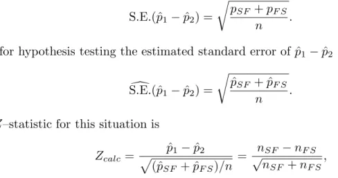
Given a simple random sample ofnresponse pairs we can use the observed proportions of (S,F) and (F,S) pairs ˆpSF and ˆpF S to estimate the standard error of ˆp1−pˆ2.
For confidence estimation the estimated standard error of ˆp1 −pˆ2 is
d S.E.(ˆp1−pˆ2) = r ˆ pSF + ˆpF S−(ˆpSF −pˆF S)2 n .
The 95% margin of error of pˆ1−pˆ2 is
M.E.(ˆp1−pˆ2) = 1.96S.E.(ˆd p1−pˆ2)
and the interval from (ˆp1 −pˆ2)−M.E.(ˆp1 −pˆ2) to (ˆp1 −pˆ2) + M.E.(ˆp1 −pˆ2) is a 95%
6.4 Inference for two proportions (paired samples) 131 When computing theP–value for a hypothesis test we will assume thatp1 =p2 which
is equivalent to assuming thatpSF =pF S. Under this assumption the population standard
error of ˆp1−pˆ2 simplifies to
S.E.(ˆp1−pˆ2) =
r
pSF +pF S
n .
Thus for hypothesis testing the estimated standard error of ˆp1−pˆ2 is
d S.E.(ˆp1−pˆ2) = r ˆ pSF + ˆpF S n .
The Z–statistic for this situation is Zcalc = ˆ p1−pˆ2 p (ˆpSF + ˆpF S)/n = √nSF −nF S nSF +nF S ,
where nSF and nF S are the respective frequencies of (S,F) and (F,S) pairs. Notice that
this test statistic only depends on the frequencies nSF andnF S, it does not depend on the
sample size n.
Example. Instant coffee purchases. This example is based on a study described in Grover and Srinivasan, A simultaneous approach to market segmentation and market structuring,J. of Marketing Research,24May 1987, 139–153. The authors selected a sim-ple random samsim-ple of households from the 4657 households constituting the 1981 MRCA market research panel. The data summarized in Table 2 correspond to a simple random sample of n= 541 households selected from the subpopulation of the MRCA households that purchased decaffeinated instant coffee at least twice during the one year study period. These purchases are recorded as Sanka or other to indicate the brand of coffee purchased. Let p1 denote the population proportion of households that chose Sanka on the first
pur-chase and let p2 denote the population proportion of households that chose Sanka on the
second purchase.
Table 2. Instant coffee purchase data
first purchase second purchase freq. rel. freq.
Sanka Sanka 155 .2865
Sanka other 49 .0906
other Sanka 76 .1405
other other 261 .4824
541 1.0000
In this sample 37.71% of the first purchases were Sanka and 42.70% of the second pur-chases were Sanka. Note that ˆpSF = .0906 and ˆpF S = .1405 indicating that 9.06% of
132 6.4 Inference for two proportions (paired samples)
the households switched from Sanka to other and 14.05% of the households switched from other to Sanka. In this case ˆp1 −pˆ2 = .3771−.4270 = −.0499, the standard error for
estimation is d S.E.(ˆp1−pˆ2) = r .0906 +.1405−(.0906−.1405)2 541 =.02056
and the 95% margin of error is M.E.(ˆp1−pˆ2) =.0403. This gives a 95% confidence interval
forp1−p2 ranging from−.0499−.0403 =−.0902 to−.0499+.0403 =−.0096. Thus we are
95% confident that the proportion of all households in the subpopulation defined above that chose Sanka first is between .0096 and .0902 smaller than the proportion of all households that chose Sanka second. In other words, for this population of decaffeinated instant coffee purchasers, we are 95% confident that the percentage of all households that chose Sanka on the second purchase is .96 to 9.02 percentage points higher than the percentage of all households that chose Sanka on the first purchase.
To demonstrate the method, consider a test of the null hypothesis H0 :p1 = p2 (the
same proportion purchase Sanka first as second) versus the research hypothesisH1 :p1 6=p2
(the proportions are different). For this test the Z–statistic is Zcalc = nSF −nF S √ nSF +nF S = √49−76 49 + 76 =−2.4150
and the P–value is P(Z ≤ −2.415) +P(Z ≥2.415) =.0157. Therefore, there is sufficient evidence to conclude that p1 and p2 are different.
Another situation where an inference about p1−p2 is based on dependent estimates
ˆ
p1 and ˆp2 arises when a single sample of units is categorized into three or more categories.
Suppose that three or more candidates are listed on a ballot and we want to compare the proportion of all voters who favor candidate A, pA, with the proportion of all voters who
favor candidate B, pB. Let pC = 1−(pA+pB) denote the proportion of all voters who
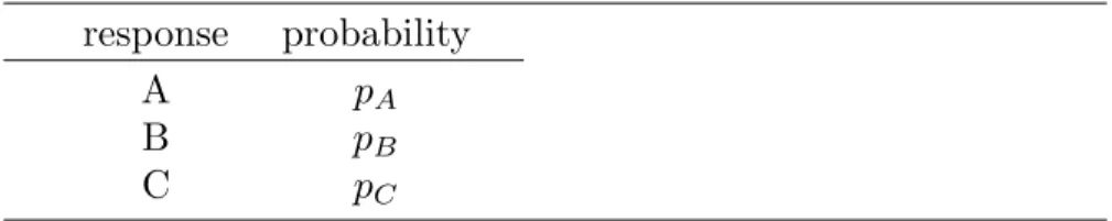
favor neither A nor B or who have no opinion. The probability model for this situation given in Table 3 is determined by the corresponding population probabilities pA, pB, and
pC. Notice that these three probabilities must sum to one.
Table 3. Probability model for trichotomous responses response probability
A pA
B pB
6.4 Inference for two proportions (paired samples) 133 Assuming that the data form a simple random sample of sizen; ˆpA, ˆpBand ˆpA−pˆB are
unbiased estimators ofpA, pB, and pA−pB. In this situation the population standard
error of ˆpA−pˆB,
S.E.(ˆpA−pˆB) =
r
pA+pB−(pA−pB)2
n ,
depends on the sample size n and the two probabilities pA and pB.
For confidence estimation the estimated standard error of ˆpA−pˆB is
d S.E.(ˆpA−pˆB) = r ˆ pA+ ˆpB−(ˆpA−pˆB)2 n ,
and the 95% margin of error of pˆA−pˆB is
M.E.(ˆpA−pˆB) = 1.96S.E.(ˆd pA−pˆB).
When computing the P–value for a hypothesis test we will assume that pA = pB.
Under this assumption the population standard error of ˆpA−pˆB simplifies to
S.E.(ˆpA−pˆB) =
r
pA+pB
n .
Thus for hypothesis testing the estimated standard error of ˆpA−pˆB is
d S.E.(ˆpA−pˆB) = r ˆ pA+ ˆpB n . The Z–statistic for this situation is
Zcalc = ˆ pA−pˆB p (ˆpA+ ˆpB)/n = √nA−nB nA+nB ,
where nA andnB are the respective frequencies of categories A and B. As in the previous
application, this test statistic only depends on the frequencies nA and nB, it does not
depend on the sample size n.
Example. Opinions about a change in tax law (revisited). Recall that a simple random sample of 100 taxpayers with telephones was selected and each taxpayer was asked “Do you favor or oppose the proposed change in state tax law?”. For this population of taxpayers let pA denote the proportion who would respond “favor”, let pB denote the
proportion who would respond “oppose”, and let pC denote the proportion who would
respond “no opinion”. When we first looked at this example we considered two ways to dichotomize this population so that we could use inferential methods for a single proportion p. First we considered “favor” versus “not favor” for the entire population and inference
134 6.5 Summary
about p = pA (with 1−p = pB +pC). Then we considered “favor” versus “oppose” for
the subpopulation of taxpayers who had an opinion and inference aboutp=pA/(pA+pB)
(with 1 −p = pB/(pA +pB)). We now have methods for making inferences about the
difference pA−pB without restricting the population.
As before, suppose thatn= 100, 64 taxpayers favor the change, 26 taxpayers oppose the change, and 10 taxpayers have no opinion. For this sample we have ˆpA = .64 and
ˆ
pB =.26, which gives the estimated standard error for estimation of
d
S.E.(ˆpA−pˆB) =
r
.64 +.26−(.64−.26)2
100 =.0869
and a 95% margin of error of .1703. Therefore, we are 95% confident that pA −pB is
between.38−.1703 =.2097 and.38 +.1703 =.5503. In other words, we are 95% confident that the actual proportion of taxpayers in this metropolitan area (who have telephones) who favored the proposed tax law change at the time of this poll is between 20.97 and 55.03 percentage points higher than the corresponding proportion who opposed the change.
To demonstrate a hypothesis test consider the research hypothesis H1 :pA > pB that
a larger proportion of all the taxpayers in this metropolitan area (who have telephones) favored the proposed tax law change at the time of this poll than opposed the change. The estimated standard error for testing is
d
S.E.(ˆpA−pˆB) =
r
.64 +.26
100 =.09487,
giving Zcalc = .38/.09487 = 4.0055 with P–value = P(Z ≥ 4.0055) = 3.1×10⁻⁵. Thus
there is very strong evidence that a larger proportion of all the taxpayers in this metropoli-tan area (who have telephones) favored the proposed tax law change at the time of this poll than opposed the change.
Remark. This hypothesis test is actually equivalent to the conditional test for the research hypothesisH1 :p > .5forp=pA/(pA+pB)when the population and sample are restricted
to the subpopulation and subsample of taxpayers who had an opinion at the time of the poll. That is, if we compute Zcalc and the P–value for n= 90 and pˆ= 64/90 = .7111 we
get Zcalc = 4.0055 and P–value = 3.1×10⁻⁵.
6.5 Summary
In this chapter we considered the use of the observed difference between two propor-tions ˆp1 −pˆ2 to make inferences about the corresponding population difference p1 −p2.
First we considered the case when the estimates ˆp1 and ˆp2 are independent. In this case
6.5 Summary 135 considered the case when the estimates ˆp1 and ˆp2 are dependent. In this case we
consid-ered two situations. First we assumed that ˆp1 and ˆp2 were computed from a single random
sample of paired observations and then we assumed that ˆp1 and ˆp2 were computed from a
single random sample from a population of units with three or more possible categorical values.
The confidence interval estimates of p1 −p2 and formal tests of hypotheses about
p1−p2 are based on a normal approximation to the sampling distribution of ˆp1−pˆ2 and
require certain assumptions about the random samples. Strictly speaking, the inferential methods discussed in this chapter are not appropriate unless these assumptions are valid. Independent estimates
For the independent estimates case the requisite assumptions are that the data consist of two independent simple random samples selected with replacement or equivalently two independent sequences of Bernoulli trials. The assumption of independent random samples is very important. We also noted that this approximation works well for independent simple random samples selected without replacement provided both of the populations being sampled are very large. The sampling distribution of ˆp1 − pˆ2 is the theoretical
probability distribution of ˆp1−pˆ2 which indicates how ˆp1 −pˆ2 behaves as an estimator
of p1−p2. Under the assumptions described above, the sampling distribution of ˆp1 −pˆ2
indicates that ˆp1−pˆ2 is unbiased as an estimator of p1−p2 (ˆp1−pˆ2 neither consistently
overestimates p1 −p2 nor consistently underestimates p1 −p2) and provides a measure
of the variability in ˆp1 −pˆ2 as an estimator of p1 −p2 (the population standard error of
ˆ
p1 −pˆ2, S.E.(ˆp1 −pˆ2) =
p
p1(1−p1)/n1+p2(1−p2)/n2 ). The normal approximation
allows us to compute probabilities concerning ˆp1−pˆ2 by re–expressing these probabilities
in terms of the standardized variable Z = [(ˆp1−pˆ2)−(p1−p2)]/S.E.(ˆp1−pˆ2) and using
the standard normal distribution to compute the probabilities.
A 95% confidence interval estimate of p1 −p2 is an interval of plausible values for
p1 − p2 constructed using a method which guarantees that 95% of such intervals will
actually contain the unknown difference p1 −p2 between the population proportions. In
the present context a confidence interval forp1−p2may include only negative numbers, only
positive numbers, or a mixture of negative and positive numbers, since we are estimating a difference. The 95% confidence interval estimate of p1 −p2 is formed by adding and
subtracting the appropriate margin of error to an estimate of p1 −p2. The estimate is
ˆ
p1−pˆ2 and the margin of error M.E.(ˆp1−pˆ2) used to form the 95% confidence interval is
M.E.(ˆp1−pˆ2) = 1.96 s ˆ p1(1−pˆ1) n1 + pˆ2(1−pˆ2) n2 .
136 6.5 Summary
The 95% confidence interval is the interval from (ˆp1−pˆ2)−M.E.(ˆp1 −pˆ2) to (ˆp1−pˆ2) +
M.E.(ˆp1 −pˆ2). Notice that the margin of error of ˆp1 −pˆ2 is a constant multiple (the
multiplier is 1.96) of the estimated standard error of ˆp1−pˆ2,
d S.E.(ˆp1−pˆ2) = s ˆ p1(1−pˆ1) n1 + pˆ2(1−pˆ2) n2 .
We also discussed formal hypothesis tests to compare two competing, complementary hypotheses (the null hypothesis H0 and the research or alternative hypothesis H1) about
p1−p2. Recall that a hypothesis test begins by tentatively assuming that H0 is true and
examining the evidence, which is quantified by the appropriate P–value, against H0 and
in favor of H1. Since the P–value quantifies evidence against H0 and in favor of H1, a
small P–value constitutes evidence in favor of H1. Guidelines for interpreting a P–value
are given on page 99.
If there is sufficient a priori information to specify a directional hypothesis of the form H1 : p1 −p2 > 0 or H1 : p1 −p2 < 0, then we can perform a hypothesis test to
address the respective questions “Is there sufficient evidence to conclude that p1 > p2
(p1−p2 > 0)?” or “Is there sufficient evidence to conclude that p1 < p2 (p1 −p2 < 0)?”
The null hypotheses for these research hypotheses are their negations H0 : p1 ≤ p2 and
H0 : p1 ≥ p2, respectively. The hypothesis test proceeds by tentatively assuming that
the null hypothesis H0 is true and checking to see if there is sufficient evidence (a small
enough P–value) to reject this tentative assumption in favor of the research hypothesis H1. The P–values for these directional hypothesis tests are based on the observed value
of the Z–statistic Zcalc = ˆ p1−pˆ2 d S.E.(ˆp1−pˆ2) , where, in this testing context, the estimated standard error is
d S.E.(ˆp1−pˆ2) = s ˆ p(1−p)ˆ 1 n1 + 1 n2 ,
with ˆp denoting the proportion of successes in the combined sample of all n1+n2 units.
ForH1 :p1 > p2 large values of ˆp1−pˆ2, relative to zero, favor H1 overH0 and theP–value
is the probability that Z ≥ Zcalc. For H1 : p1 < p2 we look for small values of ˆp1−pˆ2,
relative to zero, and the P–value is the probability that Z ≤Zcalc.
For situations where there is not enough a priori information to specify a directional hypothesis we considered a hypothesis test for the null hypothesisH0 :p1 =p2 versus the
alternative hypothesis H1 : p1 6= p2. Again we tentatively assume that H0 is true and
6.6 Exercises 137 assumption in favor ofH1. In this situation the hypothesis test addresses the question “Are
the data consistent withp1 =p2 or is there sufficient evidence to conclude that p1 6=p2?”
For this non–directional hypothesis test we take the absolute value when computing the observed value of the Z–statistic
Zcalc = | ˆ p1−pˆ2| d S.E.(ˆp1−pˆ2) ,
since values of ˆp1−pˆ2 which are far away from zero in either direction support p1 6= p2
over p1 =p2. Thus theP–value for this hypothesis test is the probability that|Z| ≥Zcalc.
For all of these hypothesis tests, the P–value is computed under the assumption that H0 is true. The P–value is the probability of observing a value of ˆp1 − pˆ2 that is as
extreme or more extreme, relative to zero, than the value we actually observed, under the assumption that H0 is true (in particular ˆp1 = ˆp2). In this statement the definition of
extreme (large, small, or far from in either direction) depends on the form of H1.
Dependent estimates
For the dependent estimates case we first considered the situation when the data con-sist of a single simple random sample of success/failure pairs (or equivalently success/failure pairs corresponding to paired sequences of Bernoulli trials). We then considered the situ-ation when the data consist of a simple random sample selected with replacement from a population of units with three or more possible categorical values. The details are given in Section 6.4.
6.6 Exercises
Provide a complete analysis for each of the following examples. Be sure to: define relevant population proportions p1 and p2; setup and perform a relevant hypothesis test; and, find
a confidence interval for p1 −p2. Provide a complete summary of your findings in the
context of the example.
1. Childers and Ferrell (1979) (Journal of Marketing Research, 16, 429–431) conducted a study to investigate the effects of the format of a survey on the response rate for mailed questionnaires. In this context the response rate is the probability that a recipient will return the completed questionnaire. They created two forms of a questionnaire one with questions on both sides of a single sheet of paper and one with questions on one side of each of two sheets of paper. Before reading the remainder of this example answer the following question. Which of these two formats do you believe would result in a higher response rate and why do you believe this? Childers and Ferrell randomly divided a sample of 440 members of the American Marketing Association into two groups of 220.
138 6.6 Exercises
Of the 220 people who were sent the one sheet version of the questionnaire, 79 returned the questionnaire. Of the 220 people sent the two sheet version of the questionnaire, 66 returned the questionnaire.
2. This example is based on a study of D.M. Barnes (1988), Science, 241, 1029–1030, as described in Moore (1995). This study was conducted to compare two antidepressants as treatments for cocaine addiction. In particular, the researchers wanted to compare the effects of the antidepressant desipramine with the effects of lithium (a standard treatment for cocaine addiction). A group of 48 chronic cocaine users was randomly divided into two groups of 24. One group was treated with desipramine and the other was treated with lithium. The subjects were tracked for three years and the number of subjects who relapsed into cocaine use during this period was recorded. Ten of the 24 people in the desipramine group relapsed into cocaine use and 18 of the 24 people in the lithium group relapsed.