PALEOCLIMATE RECONSTRUCTION IN NORTHWEST SCOTLAND
AND SOUTHWEST FLORIDA DURING THE LATE HOLOCENE
Ting Wang
A dissertation submitted to the faculty of the University of North Carolina at Chapel Hill in partial fulfillment of the requirements for the degree of Doctor of Philosophy in the
Department of Geological Sciences.
Chapel Hill 2011
© 2011 Ting Wang
ABSTRACT
TING WANG: Paleoclimate Reconstruction in Northwest Scotland and Southwest Florida during the Late Holocene
(Under the direction of Dr. Donna M. Surge)
The study reconstructed seasonal climate change in mid-latitude northwest Scotland during the climate episodes Neoglacial (~3300-2500 BP) and Roman Warm Period (RWP; ~2500-1600 BP) and in subtropical southwest Florida during the latter part of RWP (1-550 AD) based on archaeological shell accumulations in two study areas. In northwest Scotland, seasonal sea surface temperature (SST) during the Neoglacial and RWP was estimated from
high-resolution oxygen isotope ratios (δ18O) of radiocarbon-dated limpet (
Patella vulgata) shells accumulated in a cave dwelling on the Isle of Mull. The SST results revealed a cooling transition from the Neoglacial to RWP, which is supported by earlier studies of pine pollen in Scotland and European glacial events and also coincident with the abrupt climate
deterioration at 2800-2700 BP. The cooling transition might have been driven by decreased solar radiation and weakened North Atlantic Oscillation (NAO) conditions. In southwest Florida, seasonal-scale climate conditions for the latter part of RWP were reconstructed by using high-resolution δ18O of archaeological shells (
and cooling trend across the RWP to Vandal Minimum (VM; ~500-800 AD) transition, which is consistent with falling sea level and reduced solar radiation. Reduced solar radiation might have triggered a change in atmospheric circulation patterns that precipitated the
ACKNOWLEDGEMENTS
I wish to thank my advisor Dr. Donna Surge for your continuous guidance and support. I cherish the enriching and nurturing experiences from you. I am also grateful to my committee, Dr. Carter, Dr. Rial, Dr. Ries and Dr. Walker, for your insightful suggestions and comments.
Last, but not least, I would like to thank my beloved mother, father, and brother in China, and especially my husband for your support and encouragement. I’m also grateful to my friends at Chapel Hill and my host family Ms. Marjorie White for your precious
friendship.
TABLE OF CONTENTS
LIST OF TABLES………...x
LIST OF FIGURES………..xi
LIST OF ABBREVIATIONS AND SYMBOLS………..xiii
Preface………xvi
References………..……..xviii
Chapter I. SEASONAL TEMPERATURE VARIABILITY OF THE NEOGLACIAL AND ROMAN WARM PERIOD RECONSTRUCTED FROM OXYGEN ISOTOPE RATIOS OF LIMPET SHELLS (PATELLA VULGATA), NORTHWEST SCOTLAND……….………...………...1
Abstract……….…...1
Keywords………2
1 Introduction.………..………..……….2
1.1 Ecology of Patella vulgata ………...………..4
1.2 Oceanography of Study Area….……….……….………5
2 Materials and methods…………...………...6
2.2 Geochemical analysis.………...7
2.3 Estimated temperature….………...8
3 Results………..………..………10
3.1 Neoglacial ………..……...10
3.2 Roman Warm Period ………...………..10
4 Discussion………..……….…...11
4.1 Neoglacial ………...11
4.2 Roman Warm Period ………...…...14
4.3 Comparison of Neoglacial and Roman Warm Period...……..16
4.4 Subboreal/Subatlantic transition ………..…...18
5 Conclusions………..…………..………21
Acknowledgements………...21
References……….………23
II. SEASONAL CLIMATE CHANGE ACROSS THE ROMAN WARM PERIOD/VANDAL MINIMUM TRANSITION USING ISOTOPE SCLEROCHRONOLOGY IN ARCHAEOLOGICAL SHELLS AND OTOLITHS, SOUTHWEST FLORIDA, USA..………...39
Abstract……….………...39
Keywords………...40
1 Introduction.………..……….……….40
2 Study Site………...………42
2.1 Climatic context….………….……….……….……….…42
2.2 Archaeological context….………….……….………….…………..……44
3.2 Microstructure and miscrosampling..…………...46
3.3 Estimated precipitation and temperature….………….……….47
4 Results………..……...………49
5 Discussion………....…...50
5.1 Oxygen isotope ratios of shells and otoliths…...50
5.2 Reconstructed precipitation and temperature during the RWP……...51
5.3 Climate transition across the RWP and VM climate episodes...….54
6 Conclusions……….………57
Acknowledgements………..…..58
References……..………59
III. STOCHASTIC EVALUATION OF CLIMATE CHANGE OVER THE PAST 1000 YEARS………...………...73
Abstract………..………...73
1 Introduction………..……..………...………..…………74
2 Methods………...77
2.1 Stochastic climate model…...77
2.2 Randomness evaluation for stochastic time series (RESTS)...79
3 Results and discussion………81
3.1 Evaluation of stochastic extent with linear stochastic climate model…....81
3.2 Temporal variations of stochastic extent over the past millennium……...84
4 Conclusions……….………87
Acknowledgements………..…………..88
References………..……89
LIST OF TABLES
Table
1.1. Time range of the archaeological limpets.………..………29 1.2. Summary statistics for temperature estimated from the Neoglacial
limpets...30 1.3. Summary statistics for temperature estimated from the Roman Warm
Period limpets...31 2.1. Time range of the archaeological shells in the Roman Warm Period…………..63 2.2. Summary statistics for the modern and Roman Warm Period shells and
LIST OF FIGURES
Figure
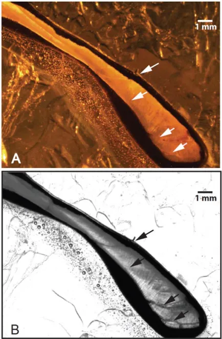
1.1. Map of Scotland and Isle of Mull.………..………...…...32 1.2. Cross-section along the axis of maximum growth of archaeological
limpet 102b-43-1...33
1.3. δ18O values of the Neoglacial limpets versus distance from margin
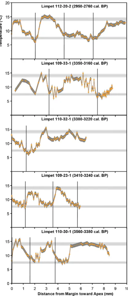
toward apex………...34 1.4. Estimated temperatures with errors from the Neoglacial limpets...…….35
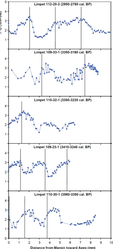
1.5. δ18O values of the Roman Warm Period limpets versus distance from
margin toward apex....………...……….……….……….36 1.6. Estimated temperatures with errors from the Roman Warm Period
limpets………...37 1.7. Temperature comparison between the Neoglacial and Roman Warm
Period……….………..……….…...38 2.1. Map and stratigraphy of the study area...………...………..67 2.2. Microstructure and microsampling of archaeological specimens………68
2.3. δ18O values of archaeological shells versus distance from growth
margin.…..……….………...69
2.4. δ18O values and estimated temperatures of archaeological otoliths
versus distance from the inner core toward the growth margin…...…………...70 2.5. Reconstructed Roman Warm Period and Vandal Minimum summers
and winters in comparison with sea-level change...………...……...71 2.6. Reconstructed Roman Warm Period and Vandal Minimum summers
and winters in comparison with solar irradiance change.…...………...72 3.1. Temperature variations of Northern Hemisphere over the past
millennium………...92 3.2. Comparison between the reconstruction and the ensemble average of
3.3. Comparison between the reconstruction and the simulation with solar
forcing…………..………...94 3.4. Calibration of the method RESTS………...95 3.5. Different climate records and their score distribution with the method
LIST OF ABBREVIATIONS AND SYMBOLS
AD Anno Domini
A. felis Ariopsis felis
AMO Atlantic Multidecadal Oscillation AMS accelerator mass spectrometry AO Arctic Oscillation
BC Before Christ BP before present
CALIB calibration program for radiocarbon age 14C radiocarbon isotope 14
CIIA cultural period of Caloosahatchee IIA CI cultural period of Caloosahatchee I CI-A Caloosahatchee I-Ariopsis felis CIIA-A Caloosahatchee IIA-Ariopsis felis
CIIA-M Caloosahatchee IIA-Mercenaria campechiensis CI-M Caloosahatchee I-Mercenaria campechiensis cm centimeter
CR Citrus Ridge oC degrees Celsius
δ13C carbon isotope ratio
δ18O oxygen isotope ratio
et al. and others
FLMNH Florida Museum of Natural History
GISS GCM Goddard Institute for Space Studies general circulation model GISP2 Greenland Ice Sheet Project 2
i.e., that is
ITCZ Intertropical Convergence Zone LIA Little Ice Age
LM Low Mound Lv Level
M. camphechiensis Mercenaria campechiensis M. mercenaria Mercenaria mercenaria
μg microgram, 10-6 gram mm millimeter
MWP Medieval Warm Period
ΝΑΟ North Atlatic Oscillation
NBS National Bureau of Standard NH Northern Hemisphere
NOAA National Oceanic and Atmospheric Administration NOSAMS National Ocean Sciences Accelerator Mass Spectrometry NWP Northwest Pasture
OM Old Mound
‰ per mil or parts per thousand ± plus or minus
psu practical salinity units
P. vulgate Patella vulgata
RESTS randomness evaluation for stochastic time series RWP Roman Warm Period
SCR Surf Clam Ridge SP South Pasture SPG sub-polar gyres
SST sea surface temperature St Stratum
STG sub-tropical gyres TSI total solar irradiance VM Vandal Minimum
VPDB Vienna Pee Dee Belemnite
PREFACE
Climate in the late Holocene (0-3000 BP) was more variable and dynamic than previously thought. Several climate change episodes have been detected, such as the Subboreal/Subatlantic transition (2800-2700 cal. BP), Roman Warm Period (RWP; ~2500-1600 cal. BP), Vandal Minimum (VM; ~400-800 AD), Medieval Warm Period (MWP; ~1200-1400 AD) and Little Ice Age (LIA; ~1500-1700 AD). Paleoclimate reconstructions during these climate episodes in the sensitive North Atlantic sector are pivotal for
understanding natural variation in the climate system prior to anthropogenic influence. However, the majority of Holocene climate proxies in the North Atlantic sector provide decadal or annual resolution. Few studies provide the high resolution necessary to reconstruct seasonal-scale variability, which can provide more accurate reconstruction necessary to gain insights into climate mechanism. Therefore, there is an increasing demand for seasonal-scale resolution.
understanding of human-climate relationships (Surge and Walker, 2005; Walker and Surge, 2006; Hallmann et al., 2009; Hufthammer et al., 2010; Jones et al., 2010; Patterson et al., 2010; Helama and Hood, 2011; Wang et al., 2011). The archaeological middens found along the northwest coast of Scotland and the southwest coast of Florida contain abundant shells, providing a rich source of seasonal climate records and information on human subsistence strategies. Chapter 1 reconstructs seasonal sea surface temperature (SST) variability during the Neoglacial (3300-2500 BP) and the RWP using δ18O values of archaeological limpet (Patella vulgata) shells from Croig Cave, an archaeological site in northwest Scotland. Chapter 2 reconstructs the variability of summer precipitation and winter temperature during
the latter part of RWP (1-500 AD) using δ18O values of archaeological shell-otolith pairs (Mercenaria campechiensis and Ariopsis felis) from southwest Florida.
Although solar radiation change has generally been accepted as the external trigger for climate change in the late Holocene, there is no consensus on the internal mechanism for the changes. Stochastic climate models have been widely used to help understand the
References
Ditlevsen PD. 2001. Stochastic climate dynamics observed in an ice-core record. Proceedings ISSAOS 2001, l'Aquilla.
Dobrovolski SG. 2000. Stochastic climate theory: models and applications. Springer-Verlag Berlin: Heidelberg New York.
Goewert AE, Surge D. 2008. Seasonality and growth patterns using isotope sclerochronology in shells of the Pliocene scallop Chesapecten madisonius. Geo-Marine Letters 28: 327-338. Hallmann N, Burchell M, Schöne BR, Irvine GV, Maxwell D. 2009. High-resolution sclerochronological analysis of the bivalve mollusk Saxidomus gigantea from Alaska and British Columbia: Techniques for revealing environmental archives and archaeological seasonality. Journal of Archaeological Science 36: 2353-2364.
Helama S, Hood BC. 2011. Stone Age midden deposition assessed by bivalve
sclerochronology and radiocarbon wiggle-matching of Arctica islandica shell increments. Journal of Archaeological Science 38(2): 452-460.
Hufthammer AK, Høie H, Folkvord A, Geffen AJ, Andersson C, et al. 2010. Seasonality of human site occupation based on stable oxygen isotope ratios of cod otoliths. Journal of Archaeological Science 37: 78-83.
Jones KB, Hodgins GWL, Etayo-Cadavid MF, Andrus CFT, Sandweiss DH. 2010. Centuries of marine radiocarbon reservoir age variation within archaeological Mesodesma donacium shells from southern Peru. Radiocarbon 52(3): 1207-1214.
Jones D., Allmon WD. 1995. Records of upwelling, seasonality and growth in stable-isotope profiles of Pliocene mollusk shells from Florida. LETHAIA 28: 61-74.
Király A, Jánosi IM. 2002. Stochastic modeling of daily temperature fluctuations. Physical Review 65: 051102, doi: 10.1103/PhysRevE.65.051102.
Majda AJ, Timofeyev I, Eijnden EV. 1999. Models for stochastic climate prediction. PNAS 96: 14687-14691, doi: 10.1073/pnas.96.26.14687.
Patterson WP, Dietrich KA, Holmden C, Andrews JT. 2010. Two millennia of North Atlantic seasonality and implications for Norse colonies. Proceedings of the National Academy of Sciences 107 (12): 5306-5310.
Schöne BR, Fiebig J, Pfeiffer M, Gleβ R, Hickson J, Johnson ALA, Dreyer W, Oschmann W. 2005. Climate records from a bivalved Methuselah (Arctica islandica, Mollusca; Iceland). Palaeography, Palaeoclimatology, Palaeoecology 228: 130-148.
Surge D, Walker K J. 2005. Oxygen isotope composition of modern and archaeological otoliths from the estuarine hardhead catfish (Ariopsis felis) and their potential to record low-latitude climate change. Palaeogeography, Palaeoclimatology, Palaeoecology 228: 179-191. Surge D, Walker KJ. 2006. Geochemical variation in microstructural shell layers of the southern quahog (Mercenaria campechiensis): Implications for reconstructing seasonality. Palaeogeography, Palaeoclimatology, Palaeoecology 237: 182-190.
Walker KJ, Surge D. 2006. Developing oxygen isotope proxies from archaeological sources for the study of Late Holocene human–climate interactions in coastal southwest Florida. Quaternary International 150: 3-11.
CHAPTER I
SEASONAL TEMPERATURE VARIABILITY OF THE NEOGLACIAL
AND ROMAN WARM PERIOD RECONSTRUCTED FROM OXYGEN
ISOTOPE RATIOS OF LIMPET SHELLS (PATELLA VULGATA),
NORTHWEST SCOTLAND
Abstract
Seasonal SST variability for the Neoglacial (3300-2500 BP) and Roman Warm Period (RWP; 2500-1600 BP), which correspond to the Bronze and Iron Ages, respectively was estimated using oxygen isotope ratios obtained from high-resolution samples micromilled from radiocarbon-dated, archaeological limpet (Patella vulgata) shells. The coldest winter months recorded in Neoglacial shells averaged 6.6±0.3ºC, and the warmest summer months averaged 14.7±0.4ºC. One Neoglacial shell captured a year without a summer, which may have resulted from a dust veil from a volcanic eruption in the Katla volcanic system in Iceland. RWP shells record average winter and summer monthly temperatures of 6.3±0.1oC and 13.3±0.3ºC, respectively. These results capture a cooling transition from the Neoglacial to RWP, which is further supported by earlier studies of pine pollen in Scotland and
European glacial events. The cooling transition observed at the boundary between the
Keywords: oxygen isotope, Patella vulgata, Neoglacial, Roman Warm Period, northwest Scotland, Subboreal/Subatlantic transition
1. Introduction
Pre-industrial climate reconstructions during the mid to late Holocene provide the necessary information for understanding natural variation in the climate system prior to anthropogenic changes in the atmosphere, hydrosphere, and land use. Moreover,
paleoclimate reconstructions that use archaeological sources contribute to our understanding of human-climate relationships (Surge and Walker, 2005; Walker and Surge, 2006; Hallmann et al., 2009; Hufthammer et al., 2010; Jones et al., 2010; Patterson et al., 2010; Helama and Hood, 2011; Wang et al., 2011), particularly in regions that are sensitive to climate change, such as mid-latitude coastal areas of the North Atlantic. These paleoclimate records can be compared to proxies of possible climate forcings (e.g., solar activity, the North Atlantic Oscillation, Atlantic Meridional Overturning Circulation) and to predictions made by regional climate models (Shindell et al., 2001; Renssen et al., 2006; Swindles et al., 2007; Mann et al., 2009, and many others). Linking paleoclimate records with proxies of climate forcings is particularly important for the North Atlantic sector because the North Atlantic plays a critical role in heat transport and climate change at regional and global scales.
need for such high-resolution, seasonality studies. Numerical (idealized multi-level primitive equation) and sensitivity (ECBilt-Clio) model experiments show that small changes in the coupled atmospheric-oceanographic climate system influence regional mid-latitude seasonality in the North Atlantic sector (Lee and Kim, 2003; van der Schrier et al., 2007). Therefore, climate archives capable of capturing seasonal-scale resolution can provide the data necessary to gain insights into the mechanisms controling seasonal variability at mid latitudes in the North Atlantic.
In this study, we reconstructed the seasonal SST variability during the Neoglacial (3300-2500 BP) and the RWP (RWP; 2500-1600 BP) using oxygen isotope ratios of ten archaeological P. vulgata shells from Croig Cave, an archaeological site on the Isle of Mull in the Hebrides Islands west of mainland Scotland. We also compared our reconstructed temperatures with previous climate reconstructions to discuss the potential forcing factors responsible for the two climate change episodes. Based on results of climate modeling experiments (Lee and Kim, 2003; van der Schrier et al., 2007), our approach allowed us to test the hypothesis that seasonal temperature should also change when climate forcing drives climate change from one episode to the other one.
1.1. Ecology of Patella vulgata
The common European limpet, P. vulgata, is a gastropod that inhabits rocky
shorelines in the high intertidal and shallow subtidal zones. This species grazes on diatoms, algae, algal spores, and small plants from the substratum. It rarely shows migratory
movements much beyond its home base and is able to record environmental conditions at a fixed location. P. vulgata occurs in the cold- and warm-temperate biogeographic provinces from Norway to northern Spain and is particularly widespread around the British Isles (Blackmore, 1969). Water temperature and salinity tolerances of P. vulgata range from −8.7 to 42.8oC and 20 to 35 psu (practical salinity units) (Crisp, 1965; Branch, 1981), although shell growth rate slows down at extreme temperatures. Although they can inhabit a range of salinities, our specimens came from fully marine environments where surface salinity
P. vulgata has a conical, cap-shaped shell (~2-4 cm in length on average), which the apex of the shell located at the center or slightly anterior. The shell exterior exhibits gray to white color similar to the substratum, and the coarse surface is sculptured with radiating ribs and concentric growth rings. The shell interior is smooth and exhibits a prominent muscle scar. The shell cross-section reveals its major sclerochronological features, such as annual growth lines and growth increments. When the cross-section is processed with Mutvei’s solution (Schöne, et al., 2005), the sclerochronological features are enhanced and more detailed microstructures can be observed, such as semidiurnal, lunar daily, fortnightly growth lines and increments (Fenger et al., 2007). The growth rate of P. vulgata shells is not constant throughout the year and varies from 0.005mm/month to 2.6mm/month (Blackmore, 1969; Ekaratne and Crisp, 1984). Growth rate is primarily controlled by temperature. In mid to high latitudes, such as the United Kingdom, shells form a prominent growth line in the coldest winter month. In contrast, shells in low latitudes, such as the Mediterranean, slow their growth rate during the summer (Schifano and Censi, 1986). Although temperature plays the dominant role on growth rate and the formation of annual growth lines (Blackmore, 1969), reproduction can also influence growth rate (Ekaratne and Crisp, 1984).
1.2. Oceanography of study area
strength of the prevailing winds is largely governed by the North Atlantic Oscillation (NAO). During positive NAO phases, a large sea-level pressure gradient between the subtropical Azores High and the subpolar Icelandic Low will generate strong mid-latitude westerly winds and bring warm and saturated air masses northward to this region (Hurrell, 1995). The close relationship between the climate and NAO pattern has been indicated by the residual winter flows through Tiree Passage (56o37.7’N, 6o23.8’W, Fig. 1.1). Inall et al. (2009) measured the residual winter flow through Tiree Passage from 1980 to 2006 and found that winter flow has significant correlation with the NAO index.
The coastal waters in our study area are dominantly marine with a narrow (±0.3 psu) salinity range around 34.3 psu (Inall et al., 2009). The coastal waters are primarily composed of two sources: the Scottish Coastal Current from the Irish and Clyde Seas and the North Atlantic Current from Atlantic origin. Inall et al. (2009) reported that ~50% of the
temperature variance is attributed to the temperature variations of Irish and Clyde Sea waters, and ~17% of the variance to that of the North Atlantic Current.
2. Materials and methods
2.1. Archaeological site, shell selection and radiocarbon dating
Ages and spans the Neoglacial through Little Ice Age climate episodes. The midden deposits of Croig Cave were first excavated in 2006 and were further explored in 2007.
Bulk samples were collected from discrete stratigraphic horizons, and shells were hand picked from bulk samples for radiocarbon dating. Shells were selected based on growth rate, preservation (diagenetic assessment), and pristine taphonomic grade. Only specimens with >1mm of growth per year were used to avoid truncated records (i.e., diminished amplitudes in the δ18O time series) due to slow ontogenetic growth (e.g., Fig. 5 in Fenger et al., 2007). Assessment of diagenetic alteration requires preservation of original mineralogy. We selected shells with original calcitic microstructure (concentric cross-foliated and radial cross-foliated layers) indicating fidelity of the stable isotopic ratios. Shells containing remnants of encrusting or boring organisms were not selected to avoid secondary calcite contamination (taphonomic assessment).
The selected shells were dated by accelerator mass spectrometry (AMS) at Beta Analytic Inc. in the United Kingdom. Radiocarbon dates of the archaeological shells were calibrated using MARINE04 of CALIB 6.0 (Hughen et al., 2004) and corrected for the global ocean reservoir effect (408 years), local reservoir effect (−68±6 years; Harkness, 1983), and 13C fractionation (Stuiver et al., 2005) (Table 1.1). We identified 5 shells (110-30-1, 109-23-1, 110-32-109-23-1, 109-33-109-23-1, 112-20-2) from the Neoglacial climate episode and 5 shells (103a-37-1, 103a-39-(103a-37-1, 111-31-(103a-37-1, 103a-38-(103a-37-1, 102b-43-1) from the RWP (Table 1.1).
Selected shells were coated with a quick-dry metal epoxy resin (J-B KWIK WELD) on the outer and inner surface to prevent the shells from breaking during cutting. The shells were sectioned from the anterior to posterior margins along the axis of maximum growth and mounted on microscope slides. The slides were attached to a Buehler Isomet low speed saw
and cut into ~1 mm thick cross-sections. Cross-sections were polished down to 1μm diamond suspension grit until the internal growth lines and increments were visible. We identified prominent annual growth lines to guide our microsampling strategy by using an Olympus stereomicroscope with a 12.5 megapixel DP71 digital camera. The light control of the
stereomicroscope allows viewing with reflected (Fig. 1.2A) and transmitted light (Fig. 1.2B). Transmitted light enhanced the prominence of winter growth lines enabling identification of these annual features to guide microsampling (Fig. 1.2B).
Limpet shells were microsampled at 20-26 samples per year from the margin toward the apex to achieve submonthly resolution. Microsampling was conducted on a Merchantek micromill with a carbide dental scriber (Brasseler). Oxygen isotope ratios of carbonate powder were measured using an automated carbonate preparation device (Kiel-III) coupled to a gas-ratio
mass spectrometer (Finnigan MAT 252) housed in the Environmental Isotope Laboratory at the
University of Arizona. The precision of the measurements was better than ±0.1‰ VPDB
(Vienna Pee Dee Belemnite) for δ18O (1σ).
2.3. Estimated temperature
1.01‰ was subtracted from each δ18O value to account for the predictable vital effect in
P.
vulgata. Calculated temperatures from the subtracted values were based on the equilibrium fractionation equation for calcite and water (Friedman and O’Neil, 1977) modified from Tarutani et al (1969):
1000lnα = 2.78 × 10⁶/T2 − 2.89
where α is the fractionation factor between calcite and water, and T is temperature in Kelvin.
The relationship between α and δ is as follows:
α = (δ18Ο
CALCITE + 1000) / (δ18ΟWATER + 1000)
where δ is expressed relative to the standard VSMOW (Vienna-Standard Mean Ocean
Water). δ18Ο
CALCITE values of limpet shells were converted from the VPDB scale to the VSMOW scale before applying the above equations using the following relationship reported by Coplen et al. (1983) and Gonfiantini et al. (1995)
δ18O
VPDB = (δ18OVSMOW − 30.91)/1.03091
because the annual mean seawater oxygen isotope ratio in the study area is similar to that of Fenger et al.(2007)’s location according to the global gridded data set of LeGrandeand Schmidt(2006). This value is reasonable because it is close to the estimation from the
salinity:δ18Ο
WATER relationship (mixing line) in nearby Loch Sunart (Austin and Inall, 2002; Fig. 1.1). The δ18Ο
WATER mixing line for Loch Sunart indicated that at 34 psu, the δ18ΟWATER value is approximately 0.12‰, in agreement with our assumed value from LeGrandeand
Schmidt(2006). Estimated temperature from the measured δ18O
SHELL values and the assumed +0.1‰±0.04‰ (VSMOW) of δ18Ο
WATER has an overall error of ±0.6ºC.
3. Results 3.1. Neoglacial
All Neoglacial shells (110-30-1, 109-23-1, 110-32-1, 109-33-1, 112-20-2) have a
temporal variation of δ18Ο values following a quasi-sinusoidal trend (Fig. 1.3). The
prominent growth lines occur at or near peaks in the δ18Ο time series. Distances between growth lines measured around 2mm except specimen 109-33-1 which measured around 4mm (Fig. 1.3 and 1.4, Table 1.2). Estimated warmest summer temperatures range from 12.6oC to 15.7oC (Fig. 1.4, Table 1.2). Estimated coldest winter temperatures of the two
chronologically youngest shells (110-30-1, 109-23-1) recorded the coldest winter
temperature around 7.0oC, whereas the three more recent shells (110-32-1, 109-33-1, 112-20-2) recorded cooler temperatures during the coldest winter months (Fig. 1.4, Table 1.112-20-2).
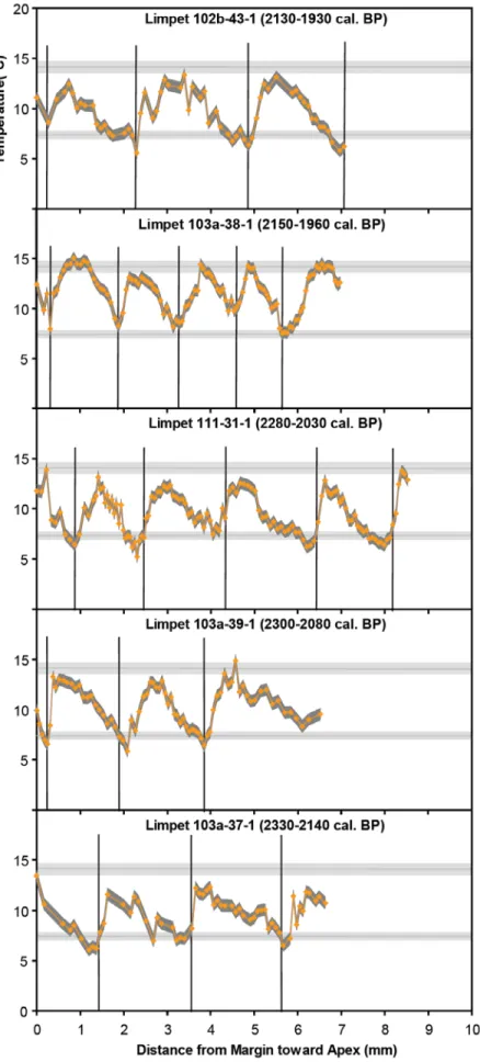
The δ18Ο values of the RWP limpets vary sinusoidally with prominent growth lines
occurring at or near the most positive δ18Ο values (Fig. 1.5). Distances between growth lines
ranged from 1.04 to 2.56 mm, although most of them are close to 2mm except specimen 103a-38-1 (Figs. 1.5 and 1.6, Table 1.3). Estimated warmest summer temperatures range from 11.6oC to 14.9oC (Fig. 1.6, Table 1.3). Coldest winter temperatures in all shells showed a consistent trend with the exception of specimen 103a-38-1 which recorded ~2oC warmer winter temperature (Fig. 1.6, Table 1.3).
4. Discussion 4.1. Neoglacial
The Neoglacial climate interval is conventionally defined as the advancing of continental glaciers following the retreat of the Wisconsin glaciation during the early
In our study, the temporal variation of δ18Ο values in Neoglacial shells (110-30-1,
109-23-1, 110-32-1, 109-33-1, 112-20-2) recorded seasonal temperature changes during the Neoglacial (Fig. 1.3). The most positive δ18Ο values represent winter, whereas the lowest
δ18Ο values represent summer. Prominent annual growth lines formed during cold winter
months (Figs. 1.3 and 1.4), which is consistent with the modern calibration study of Fenger et
al. (2007). We also observed fewer numbers of δ18Odata points in cold seasons relative to
warm seasons, reflecting slower growth during winter and fast growth during the warm
months. Both these observations are in agreement with previous studies that P. vulgata from the cold-temperate biogeographic province slows its growth during the winter (Blackmore, 1969; Jenkins and Hartnoll, 2001).
The temporal variation of δ18Ο values also showed differences among individuals.
Specimen 112-20-2 exhibited the smoothest sinusoidal curve. Specimens 109-23-1, 110-30-1 and 110-32-1 are generally smooth with several fluctuations interrupting the sinusoidal curve. Specimen 109-33-1 has the most fluctuations and therefore least smooth. These high-frequency fluctuations likely reflect frequent changes in SST rather than changes in
δ18ΟWATER because the study area is not affected by influxes of freshwater and is dominated by well-mixed shelf water (Connor et al, 2006). Perhaps these fluctuations represent times of increased storminess.
One shell (specimen 112-20-2) recorded a year (~4.58-7.09 mm from margin) lacking
the typical seasonal variation (Fig. 1.4). Normally, the δ18Ο values between two neighboring
the warmest summer. However, the third annual growth increment from the margin of specimen 112-20-2 exhibited only a slight change in temperature. We interpret this observation as a year without a summer. Such an event has been documented in 536 AD, within the Vandal Minimum climate episode. Historical documents report a widespread dust veil event that caused dimming and cooling across much of the Northern Hemisphere
(Stothers and Rampino, 1983; Rampino et al., 1988). In some regions, dry fog or aerosols were so persistent that the fine dust existed in the atmosphere for as long as 18 months. Due to the extended residence time of the dry fog or aerosols, the solar radiation was reduced to one tenth of normal and the year 536 AD was a year without summer (Gunn, 2000). In addition to the historical records, Larsen et al. (2008) reported evidence from Greenland and Antarctic ice cores suggesting that the dust veil causing the year without a summer in 536 AD resulted from a large explosive eruption from an equatorial volcano. This episode in 536 AD likely surpassed the severity of the cold period following the Tambora eruption in 1815. We hypothesize a similar cause for the year without a summer in specimen 112-20-2. The age range of specimen 112-20-2 is 2950-2760 cal. BP and is close to the time of GB4-150 tephra (2750-2708 cal. BP) identified from a peat deposit in Northern Ireland (Swindles et al., 2007). The GB4-150 tephra preserved in the Irish peat is believed to correspond to a large volcanic eruption in the Katla volcanic system in Iceland identified by Larsen et al. (2001) and Swindles et al. (2007).
on the temperature record from the National Oceanic and Atmospheric Administration (NOAA) Extended Reconstructed SST V2 database (http://www.cdd.noaa.gov). The
comparison between the estimated temperatures from the Neoglacial shells and modern SST record indicated that the coldest winter temperatures during the Neoglacial were similar to the late 20th century in the beginning of Neoglacial as recorded by the specimens 110-30-1 and 109-23-1(Fig. 1.4, Table 1.2). Following this earlier interval, the coldest winter
temperatures became ~1oC colder than the late 20th century (Fig. 1.4, Table 1.2). In the early part of our Neoglacial record, the warmest summer temperatures were ~1oC warmer than the late 20th century, subsequently became slightly colder (at the time of specimen 109-23-1), and then became warmer again (at the time of 110-32-1 and 109-33-1). The latest part of our Neoglacial summer temperature record was similar to the late 20th century (Fig. 1.4, Table 1.2). The observed temperature fluctuations are in agreement with temporal fluctuations of the pollen record from south of the Alps during the Neoglacial (Tinner et al., 2003). Aside from the temperature fluctuations, the average winter temperature for the overall Neoglacial period was 6.6±0.3ºC based on the estimated winter temperatures of all our specimens, and the average summer temperature was 14.7±0.4ºC (Table 1.2). Our results indicated that the Neoglacial winters were slightly colder than the late 20th century winters and Neoglacial summers were slightly warmer than the late 20th century summers.
4.2. Roman Warm Period
Qinghai-Tibet Plateau (Ji et al., 2005), 2700-1600 BP in southwest Greenland (Seidenkrantz et al., 2007) and 2600-1600 BP in southern Spain (Martín-Puertas et al., 2009). The character of this climate change is not always warm; for instance, the record from Martín-Puertas et al. (2009) suggests wet and humid climate during this time.
The sinusoidal time series of δ18Ο values recorded in the RWP shells reflect seasonal
We also compared the estimated RWP temperatures to the modern SST record from 1961 to 1990 near the study area. For the winter months, the RWP shells (not including excluded specimen 103a-38-1) were consistent in the coldest winter temperatures at ~6oC and therefore all recorded winter temperatures that were colder than the late 20th century. For the summer months, the RWP was initially ~2oC colder than the late 20th century as recorded by the specimen 103a-37-1 (Table 1.3). Summer temperature subsequently increased to 13oC at the time of 103a-39-1 and 111-31-1, but was still 1oC colder relative to the late 20th
century. At the time of 103a-38-1, the summer temperature was similar to the late 20th century and then dropped back to 13oC at the time of 102b-43-1. By averaging the temperatures of all the specimens, we concluded that the RWP winters (6.3±0.1oC) were ~1oC colder than late 20th century winters and the RWP summers (13.3±0.3oC) were slightly colder than late 20th century summers.
4.3. Comparison of Neoglacial and Roman Warm Period
As previously discussed, the five Neoglacial shells recorded average winter
temperature of 6.6±0.3ºC and average summer temperature of 14.7±0.4ºC, whereas the RWP shells recorded average winter temperature of 6.3±0.1oC and average summer temperature of 13.3±0.3oC. Therefore, the RWP winters were similar to or slightly colder than the
Neoglacial winters, and the RWP summers were ~1oC colder than the Neoglacial summers, which is statistically significant according to the results of one-way analysis of variance (F=
3.46, α=0.10, with 1 and 8 degrees of freedom). Consequently, the seasonal range of the
Our findings that the RWP was colder than the Neoglacial are consistent with
previous studies. The Neoglacial shells primarily recorded the temperature during 3500-3100 cal. BP, and most of the RWP shells recorded the temperature in 2300-1900 cal. BP (Table 1.1, Fig. 1.7). According to the pine history in Scotland (Bridge et al., 1990) and the European glacier record (Matthews and Dresser, 2008), the climate between 3500-3100 cal. BP was relatively warm compared to other times during the Neoglacial period, and the
climate between 2300-1900 cal. BP was relatively cold compared to the rest of the RWP. The macrofossil record of Scots pine (Pinus sylvestris) from Scotland indicates that the
percentage of pine pollen was high at 3520-3030 14C yr BP but decreased to a minimum at 2500-1800 14C yr BP (Bridge et al., 1990). Because pine growth requires dry, warm climate, this suggests that the RWP was colder and wetter than the Neoglacial interval; i.e., had higher effective precipitation (low temperature may reduce rates of evapotranspiration and increase wetness). Moreover, the pollen record in northeast Scotland spanning the Bronze and Iron Ages also indicates a significant increase in effective precipitation at ca. 2900 cal. BP which led to more wet mire surfaces (Tipping et al., 2008). The chronology of European Neoglacial events also showed major glacial advances around 2200-1900 cal. BP and no glacial advances between 3500-3100 cal. BP (Matthews and Dresser, 2008).
generally coincident with lower coastal salinities and westward migration of isohalines (Inall et al., 2009). The westward displacement of Scottish Coastal Current and isohalines is further determined by the strength of sub-polar gyres (SPG) and sub-tropical gyres (STG). A strong SPG results in a more east-west orientated gyre and, hence, colder and fresher water mass in the coast, whereas a strong STG results in a more south-north orientated gyre and modifies the coastal water mass towards warmer and saltier. In addition, Holliday (2003) investigated the air-sea interaction and circulation in the northeast Atlantic and suggested that the gyre circulation of SPG and STG are significantly influenced by the state of the NAO. Therefore, the cooling transition detected in our study may result from the change of NAO via
modulating the strength of SPG and STG circulation.
4.4. Subboreal/Subatlantic transition
The Neoglacial-RWP climate transition detected in our study is in agreement with the Subboreal/Subatlantic transition (2800-2700 cal. BP). This climate transition is also known as the 850 cal. BC “event” and has been identified by pollen zones, and the Bronze Age/Iron Age transition based on episodes in human history. The various names for this climate shift result from its widespread impact on global climate and vegetation distribution, and hence, on prehistoric agriculture and human society.
from continental Europe (Kilian et al., 1995; van Geel et al., 1998; Speranza et al., 2000, 2002; Blaauw et al., 2004; Swindles, et al., 2007), and from eastern North America (Brown et al., 2000; Booth et al., 2003). There is also some proxy evidence from the Andean region of South America (Heusser, 1995; van Geel et al., 2000), south-central Siberia (van Geel et al., 2004), and northwest Africa (Van Geel et al., 1998; Elenga et al., 2004). In the North Atlantic, colder surface waters and accompanying prominent increases in drift ice around 2800 cal. BP were detected from the proxy records in deep-sea sediment cores (Bond et al., 2001). Synchronous with the change of overlying surface waters, deep meridional
overturning circulation was reduced in the North Atlantic (Bianchi and McCave, 1999; Oppo et al., 2003; Hall et al., 2004). In continental Europe, this climate event shows more or less regional variation, although it is normally characterized by a decline of temperature or a wetter climate shift. Sudden increase in wet conditions started at ca. 2800 cal. BP in the eastern part of Netherlands based on high resolution AMS dating and micro/macro-fossil compositions of Holocene bog deposits (Kilian et al., 1995; Blaauw et al., 2004). A shift to wetter and cooler climate occurred at ca. 2800 cal. BP according to proxy records in the peat sequence of the Giant Mountains (Czech Republic) (Speranza et al., 2000, 2002). The multiproxy records from the peatlands of northern Ireland reveal a major climate shift to wetter/colder climate conditions at ca. 2700 cal. BP (Swindles, et al., 2007). The resolution for these proxy records is generally at the decadal scale.
irradiance probably triggered this climate shift. This hypothesis is supported by the solar activity record derived from the Δ14C record of multiple peat deposits in northwest Europe (Mauquoy et al., 2004). Renssen et al. (2006) further explored the impact of reduced solar activity on centennial-scale cooling events in the Holocene by using the coupled global atmosphere-ocean-vegetation model ECBilt-CLIO-VECODE. In the simulation, the global annual atmospheric surface temperature anomaly closely followed variations in total solar irradiance (TSI) during the cooling phase of 2800-2700 cal. BP, implying that temperature change was triggered by reduced solar activity. In addition, the simulation showed a spatial pattern in the temperature change. For instance, the strongest cooling (up to 0.5ºC) was observed at Northern Hemisphere mid-latitude continents, which is in agreement with most proxy evidence. After 2700 cal. BP, the value of the TSI anomaly started to increase, but the global atmospheric surface temperature anomaly still remained low. The extended cooling of surface temperature was explained by positive oceanic feedbacks. Simulated precipitation at Northern Hemisphere mid-latitudes did not show significant change on continents, which is inconsistent with the general shift to wetter conditions found in proxy data from continental Europe.
Moreover, Mann et al. (2009) and Trouet et al. (2009) implicated weak NAO conditions as a driver of climate during the Little Ice Age, which may also explain the cooling trend
observed in our study. However, we are not able to exclude other possibilities in explaining the cooling transition from the Neoglacial to the RWP.
5. Conclusions
Our study provides the first reconstruction of SST variability at seasonal time scales in the North Atlantic along northwestern coastal Scotland across the Neoglacial-RWP transition. Neoglacial shells recorded slightly colder winters and slightly warmer summers during their growth period. RWP shells generally have slightly colder summers and ~1oC colder winters than present during their growth period. Our findings document a slight winter cooling and a significant summer cooling of ~1ºC from the Neoglacial to the RWP. This cooling transition is supported by other paleoclimate proxies in Scotland and Europe. This transition is likely associated with the Subboreal/Subatlantic transition and may have been triggered by reduced solar radiation at 2800-2700 cal. BP with weakened NAO conditions. One shell from the Neoglacial period captured a year without a summer, which may have resulted from an explosive volcanic eruption in the Katla volcanic system in Iceland.
Acknowledgements
References
Austin WEN, Inall ME. 2002. Deep-water renewal in a Scottish fjord: temperature, salinity and oxygen isotopes. Polar Research 21: 251-257.
Baxter JM, Boyd IL, Cox M, Cunningham L, Holmes P, Moffat CF. 2008. Scotland's seas: towards understanding their state. Fisheries Research Services, Aberdeen.
Bianchi GG, McCave IN. 1999. Holocene periodicity in North Atlantic climate and deep-ocean flow south of Iceland. Nature 397: 515–517.
Blaauw M, van Geel B, van der Plicht J. 2004. Solar forcing of climatic change during the mid-Holocene: indications from raised bogs in the Netherlands. Holocene 14: 1-35. Blackmore DT. 1969. Studies of Patella vulgata L.I. Growth, reproduction, and zonal distribution. Journal of Experimental Marine Biology and Ecology 3: 200–213.
Bond G, Kromer B, Beer J, Munscheler R, Evans MN, Showers W, Hoffmann S, Lotti R, Hajdas I, Bonani G. 2001. Persistent solar influence on North Atlantic climate during the Holocene. Science 294: 2130–2136.
Booth RK, Jackson ST. 2003. A high-resolution record of late-Holocene moisture availability from a Michigan raised bog, USA. Holocene 13: 863–876.
Branch GM. 1981. The biology of limpets: Physical factors, energy flow, and ecological interactions. Oceanography and Marine Biology: an annual review 19: 235-380.
Bridge MC, Haggart BA, Lowe JJ. 1990. The history and palaeoclimatic significance of subfossil remains of Pinus sylvestris in blanket peats from Scotland. Journal of Ecology 78: 77-99.
Brown SL, Bierman PR, Lini A, Southon J. 2000. 10000 yr record of extreme hydrological events. Geology 28: 335–338.
Cohen AL, Tyson PD. 1995. Sea-surface temperature fluctuations during the Holocene off the south coast of Africa: Implications for terrestrial climate and rainfall. Holocene 5: 304-312.
Connor DW, Gilliland PM, Golding N, Robinson P, Todd D, Verling E. 2006. UKSeaMap: the mapping of seabed and water column features of UK seas. Joint Nature Conservation Committee, Peterborough.
Crisp DJ. 1965. Observations on the effect of climate and weather on marine communities. In The Biological Significance of Climatic Changes in Britain, Johnson CG, Smith LP (eds). Elsevier: New York; 63-77.
Elenga H, Maley J, Vincens A, Farrera I. 2004. Palaeoenvironments, palaeoclimates and landscape development in Atlantic Equatorial Africa: a review of key sites covering the last 25 kyrs. In Past climate variability through Europe and Afrcia, Battarbee, RW, Gasse F, Stickley CE (eds). Springer: Dordrecht; 181–198.
Ekaratne SUK, Crisp DJ. 1984. Seasonal growth studies of intertidal gastropods from shell micro-growth band measurements, including a comparison with alternative methods. Journal of the Marine Biological Association of the United Kingdom 64: 13-210.
Fenger T, Surge D, Schone B, Milner N. 2007. Sclerochronology and geochemical variation in limpet shells (Patella vulgata): A new archive to reconstruct coastal sea surface
temperature. Geochemistry Geophysics Geosystems 8: Q07001, doi:10.1029/2006GC001488. Friedman I, O’Neil JR. 1977. Compilation of stable isotope fractionation factors of
geochemical interest. In Data of Geochemistry, Fleischer M (ed). U.S. Govt. Print. Office: Washington, D.C.; 1-12.
Goewert AE, Surge D. 2008. Seasonality and growth patterns using isotope sclerochronology in shells of the Pliocene scallop Chesapecten madisonius. Geo-Marine Letters 28: 327-338. Gonfiantini R, Stichler W, Rozanski K. 1995. Standards and intercomparison materials distributed by the International Atomic Energy Agency for stable isotope measurements. In References and Intercomparison Materials for Stable Isotopes of Light Elements, the Isotope Hydrology Section of the International Atomic Energy Agency (eds). IAEA: Vienna,
Austria; 13-29.
Gunn JD. 2000. The years without summer: tracing A.D. 536 and its aftermath. British Archaeological Reports International Series 872.
Hall IR, Bianchi GG, Evans JR. 2004. Centennial to millennial scale Holocene climate-deep water linkage in the North Atlantic. Quaternary Science Reviews 23: 1529-1536.
Hallmann N, Burchell M, Schöne BR, Irvine GV, Maxwell D. 2009. High-resolution sclerochronological analysis of the bivalve mollusk Saxidomus gigantea from Alaska and British Columbia: Techniques for revealing environmental archives and archaeological seasonality. Journal of Archaeological Science 36: 2353-2364.
Hass HC. 1996. Northern Europe climate variations during late Holocene: evidence from marine Skagerrak. Palaeogeography, Palaeoclimatology, Palaeoecology 123: 121-145. Helama S, Hood BC. 2011. Stone Age midden deposition assessed by bivalve
sclerochronology and radiocarbon wiggle-matching of Arctica islandica shell increments. Journal of Archaeological Science 38(2): 452-460.
Heusser CJ. 1995. Palaoecology of a Donatia-Astlia cushion bog, Magellanic Moorland-Subantarctic Evergreen Forest transition, southern Tierra del Fuego, Argentina. Review of Paleobotany and Palynology 89: 429-40.
Holliday NP. 2003. Air-Sea interaction and circulation changes in the northeast Atlantic. Journal of Geophysical Research 108 (C8): 3259, doi:10.1029/2002JC001344.
Hufthammer AK, Høie H, Folkvord A, Geffen AJ, Andersson C, et al. 2010. Seasonality of human site occupation based on stable oxygen isotope ratios of cod otoliths. Journal of Archaeological Science 37: 78-83.
Hughen K, Baille M, Bard E, Beck J, Bertrand C, Blackwell P, et al. 2004. Marine04 Marine radiocarbon age calibration, 26–0 ka BP. Radiocarbon 46: 1059-1086.
Hurrell JW. 1995. Decadal trends in the North Atlantic Oscillation: regional temperatures and precipitation. Science 269: 676-679.
Inall M, Gillibrand P, Griffiths C, MacDougal N, Blackwell K. 2009. On the oceanographic variability of the north-west European shelf to the west of Scotland. Journal of Marine Systems 77: 210-226.
Jenkins SR, Hartnoll RG. 2001. Food supply, grazing activity and growth rate in the limpet Patella vulgata L.: A comparison between exposed and sheltered shores. Journal of
Experimental Marine Biology and Ecology 258: 123–139.
Ji J, Shen J, Balsam W, Chen J, Liu L, Liu X. 2005. Asian monsoon oscillations in the northeastern Qinghai-Tibet Plateau since the late glacial as interpreted from visible reflectance of Qinghai Lake sediments. Earth and Planetary Science Letters 233: 61-70. Jones D., Allmon WD. 1995. Records of upwelling, seasonality and growth in stable-isotope profiles of Pliocene mollusk shells from Florida. LETHAIA 28: 61-74.
Jones KB, Hodgins GWL, Etayo-Cadavid MF, Andrus CFT, Sandweiss DH. 2010. Centuries of marine radiocarbon reservoir age variation within archaeological Mesodesma donacium shells from southern Peru. Radiocarbon 52(3): 1207-1214.
Landscheidt T. 1987. Long-range forecasts of solar cycles and climate change. In Climate History, Periodicity and Predictability. Rampino MR, Sanders JE, Newman WS, Konigsson LK. (eds).Van Nostrand Reinhold: New York; 421–445.
Larsen G, Newton AJ, Dugmore AJ, Vilmundardóttir EG. 2001. Geochemistry, dispersal, volumes and chronology of Holocene silicic tephra layers from the Katla volcanic system, Iceland. Journal of Quaternary Science 16: 119-132.
Larsen LB, Vinther BM, Briffa KR, Melvin TM, Clausen HB, Jones PD, et al. 2008. New ice core evidence for a volcanic cause of the A.D. 536 dust veil. Geophysical Research Letters 35: L04708, doi:10.1029/2007GL032450.
Lee S, Kim H. 2003. The dynamical relationship between subtropical and eddy-driven jets. Journal of the Atmospheric Sciences 60: 1490-1503.
LeGrande AN, Schmidt GA. 2006. Global gridded data set of the oxygen isotopic composition in seawater. Geophysical Research Letters 33: L12604,
doi:10.1029/2006GL026011.
Mann ME, Zhang Z, Rutherford S, Bradley RS, Hughes MK, et al. 2009. Global signatures and dynamical origins of the Little Ice Age and Medieval Climate Anomaly. Science 326: 1256-1260.
Martín-Puertas C, Valero-Garcés BL, Brauer A, Mata MP, Delgado-Huertas A, Dulski P. 2009. The Iberian-Roman Humid Period (2600-1600 cal yr BP) in the Zoñar Lake varve record (Andalucía, southern Spain). Quaternary Research 71: 108-120.
Matthews JA, Dresser PQ. 2008. Holocene glacier variation chronology of the
Smørstabbtindan massif, Jotunheimen, southern Norway, and the recognition of century- to millennial-scale European Neoglacial events. Holocene 18: 181-201.
Mauquoy D, van Geel B, Blaauw M, Speranza A, van der Plicht J. 2004. Changes in solar activity and Holocene climatic shifts derived from 14C wiggle-match dated peat deposits. Holocene 14: 45-52.
Oppo DW, McManus JF, Cullen JL. 2003. Deepwater variability in the Holocene epoch. Nature 422: 277–278.
Patterson WP, Dietrich KA, Holmden C, Andrews JT. 2010. Two millennia of North Atlantic seasonality and implications for Norse colonies. Proceedings of the National Academy of Sciences 107 (12): 5306-5310.
Rampino MR, Self S, Stothers RB. 1988. Volcanic winters. Annual Review of Earth and Planetary Sciences 16: 73-99.
Renssen H, Goose H, Muscheler R. 2006. Coupled climate model simulation of Holocene cooling events: ocean feedback amplifies solar forcing. Climate of the Past 2: 79-90. Schifano G, Censi P. 1986. Oxygen and carbon isotope composition, magnesium and strontium contents of calcite from a subtidal Patella coerulea shell. Chemical Geology 58: 325-331.
Schöne BR, Fiebig J, Pfeiffer M, Gleβ R, Hickson J, Johnson ALA, Dreyer W, Oschmann W. 2005. Climate records from a bivalved Methuselah (Arctica islandica, Mollusca; Iceland). Palaeography, Palaeoclimatology, Palaeoecology 228: 130-148.
Schöne BR, Dunca E, Fiebig J, Pfeiffer M. 2005. Mutvei's solution: An ideal agent for resolving microgrowth structures of biogenic carbonates. Palaeogeography,
Palaeoclimatology, Palaeoecology 228: 149-166.
Seidenkrantz M.-S, Aagaard-Sørensen S, Sulsbrück H, Kuijpers A, Jensen KG, Kunzendorf H. 2007. Hydrography and climate of the last 4400 years in a SW Greenland fjord:
implication for Labrador Sea palaeoceanography. Holocene 17: 387-401.
Shackleton NJ. 1973. Oxygen isotope analysis as a means of determining season of occupation of prehistoric midden sites. Archaeometry 15: 133-141.
Shindell DT, Schmidt GA, Mann ME, Rind D, Waple A. 2001. Solar forcing of regional climate change during the Maunder Minimum. Science 294: 2149-2152.
Speranza A, van der Plicht J, van Geel B. 2000. Improving the time of control of the Subboreal/Subatlantic transition in a Czech peat sequence by 14C wiggle-matching. Quaternary Science Review 19: 1589-604.
Speranza A, van Geel B, van der Plicht J. 2002. Evidence for solar forcing of climate change at ca. 850 cal. BC from a Czech peat sequence. Global and Planetary Change 35: 51-65. Stothers RB, Rampino MR. 1983. Volcanic eruptions in the Mediterranean before A. D. 630 from written and archaeological sources. Journal of Geophysical Research 88: 6357-6371. Stuiver M, Reimer PJ, Reimer RW. 2005. CALIB Radiocarbon Calibration. http: //
radiocarbon.pa.qub.ac.uk/calib.
Surge D, Walker KJ. 2006. Geochemical variation in microstructural shell layers of the southern quahog (Mercenaria campechiensis): Implications for reconstructing seasonality. Palaeogeography, Palaeoclimatology, Palaeoecology 237: 182-190.
Swindles G, Plunkett G, Roe HM. 2007. A delayed climatic response to solar forcing at 2800 cal. BP: multiproxy evidence from three Irish peatlands. Holocene 17: 177-182.
Tarutani T, Clayton RN, Mayeda TK. 1969. The effect of polymorphism and magnesium substitution on oxygen isotope fractionation between calcium carbonate and water. Geochimica et Cosmochimica Acta 33: 987-996.
Tinner W, Lotter AF, Ammann B, Conedera M, Hubschmid P, van Leeuwen JFN, Wehrli M. 2003. Climatic change and contemporaneous land-use phases north and south of the Alps 2300 BC to 800 AD. Quaternary Science Reviews 22: 1447-1460.
Tipping R, Davies A, McCulloch R, Tisdall E. 2008. Response to late Bronze Age climate change of farming communities in north east Scotland. Journal of Archaeological Science 35: 2379-2386.
Trouet V, Esper J, Graham NE, Baker A, Scourse JD, Frank DC. 2009. Persistent positive North Atlantic Oscillation mode dominated the Medieval Climate Anomaly. Science 324: 78-80.
van der Schrier G, Drijfhout SS, Hazeleger W, Noulin L. 2007. Increasing the Atlantic subtropical jet cools the circum-North Atlantic. Meteorologische Zeitschrift 16: 1-8. van Geel B, Bokovenko NA, Burova ND, Chugunov KV, Dergachev VA, et al. 2004. Climate change and the expansion of the Scythian culture after 850 BC, a hypothesis. Journal of Archaeological Science 31: 1735-1742.
van Geel B, Heusser CJ, Renssen H, Schuurmans CJE. 2000. Climatic change in Chile at around 2700 BP and global evidence for solar forcing: a hypothesis. Holocene 10: 659-664. van Geel B, van der Plicht J, Kilian MR, Klaver ER, Kouwenberg JHM, Renssen H,
Reynaud-Ferrera I, Waterbolk HT. 1998. The sharp rise of Δ14C c. 800 cal BC: possible causes, related climatic teleconnections and the impact on human environments.
Radiocarbon 40: 535-550.
Walker KJ, Surge D. 2006. Developing oxygen isotope proxies from archaeological sources for the study of Late Holocene human–climate interactions in coastal southwest Florida. Quaternary International 150: 3-11.
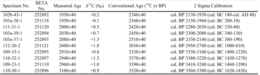
Table 1.1. Time range of the archaeological limpets.
Specimen No. BETA No. Measured Age δ13C (‰) Conventional Age (14C yr BP) 2 Sigma Calibration
102b-43-1 252892 1930±40 +0.2 2340±40 cal. BP 2130-1930 (cal. BC 180-cal. AD 40) 103a-38-1 251118 1950±40 −0.1 2360±40 cal. BP 2150-1960 (cal. BC 200-10)
111-31-1 251120 2000±40 +0.5 2420±40 cal. BP 2280-2030 (cal. BC 330-80) 103a-39-1 252894 2030±40 +0.7 2450±40 cal. BP 2300-2080 (cal. BC 340-130) 103a-37-1 252893 2080±40 +1.3 2510±40 cal. BP 2330-2140 (cal. BC 380-190) 112-20-2 251121 2600±40 +1.0 3030±40 cal. BP 2950-2760 (cal. BC 1000-810) 109-33-1 252895 2910±40 +0.8 3330±40 cal. BP 3350-3160 (cal. BC 1400-1220) 110-32-1 252897 2940±40 +1.5 3370±40 cal. BP 3380-3220 (cal. BC 1430-1270) 109-23-1 251119 2960±40 +1.0 3390±40 cal. BP 3410-3240 (cal. BC 1460-1290) 110-30-1 252896 3100±40 +0.9 3520±40 cal. BP 3560-3380 (cal. BC 1620-1430)
Table 1.2. Summary statistics for temperature estimated from the Neoglacial limpets. For each specimen, distance between growth lines, coldest winter temperature and warmest summer temperature are all listed with the first year at bottom.
Specimen (cal. BP) Distance between growth lines (mm) Coldest winter temperature (oC)
Average winter temperature with standard errors (oC)
Warmest summer temperature (oC)
Average summer temperature with standard errors (oC)
Seasonal range
(oC)
112-20-2 (2950-2760) 2.52 2.51 6.0 6.6 6.3±0.3 13.6
15.2 14.4±0.8 8.1
109-33-1
(3350-3160) 4.19
6.0
6.1 6.0
14.9
14.9 14.9 8.9
110-32-1
(3380-3220) 6.1 6.1 15.5 15.5 9.4
109-23-1 (3410-3240) 2.46 2.08 7.1 7.5 7.0 7.2±0.2 12.6
14.0 13.3±0.7 6.1
110-30-1 (3560-3380)
1.61 2.16
7.8
7.1 7.5±0.4
15.7
15 15.4±0.4 7.9
Average in
total 6.6±0.3 14.7±0.4 8.1±0.6
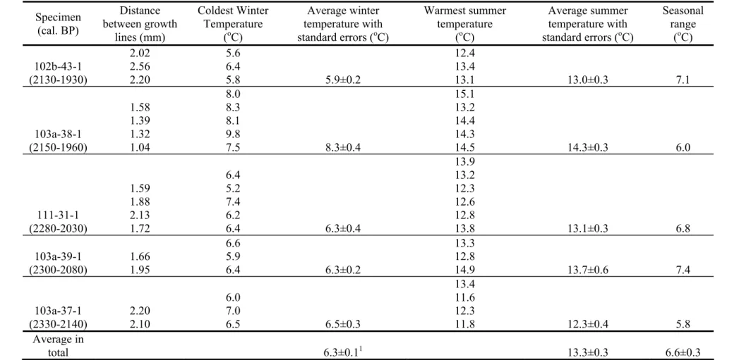
Table 1.3. Summary statistics for temperature estimated from the Roman Warm Period limpets. For each specimen, distance between growth lines, coldest winter temperature and warmest summer temperature are all listed with the first year at bottom.
Specimen (cal. BP) Distance between growth lines (mm) Coldest Winter Temperature
(oC)
Average winter temperature with standard errors (oC)
Warmest summer temperature
(oC)
Average summer temperature with standard errors (oC)
Seasonal range
(oC)
102b-43-1 (2130-1930) 2.02 2.56 2.20 5.6 6.4 5.8 5.9±0.2 12.4 13.4
13.1 13.0±0.3 7.1
103a-38-1 (2150-1960) 1.58 1.39 1.32 1.04 8.0 8.3 8.1 9.8 7.5 8.3±0.4 15.1 13.2 14.4 14.3
14.5 14.3±0.3 6.0
111-31-1 (2280-2030) 1.59 1.88 2.13 1.72 6.4 5.2 7.4 6.2
6.4 6.3±0.4
13.9 13.2 12.3 12.6 12.8
13.8 13.1±0.3 6.8
103a-39-1 (2300-2080) 1.66 1.95 6.6 5.9
6.4 6.3±0.2
13.3 12.8
14.9 13.7±0.6 7.4
103a-37-1 (2330-2140) 2.20 2.10 6.0 7.0 6.5 6.5±0.3 13.4 11.6 12.3
11.8 12.3±0.4 5.8
Average in
total 6.3±0.11 13.3±0.3 6.6±0.3
31
Figure 1.4. Estimated
temperatures with errors from the Neoglacial limpets. The vertical lines represent the positions of annual growth lines. The horizontal bars indicate the average range of summer SST data
(14.12±0.54oC) and winter SST data (7.40±0.35oC) from 1961-1990 around the grid (56oN, 6oW) provided by the National Oceanic and Atmospheric Administration (NOAA) Extended Reconstructed SST V2 database
Figure 1.6. Estimated temperatures with errors from the Roman Warm Period limpets. The vertica lines represent the position of annual growth lines. Th horizontal bars indicate the average range of summer SST data (14.12±0.54oC) and winter SST data
(7.40±0.35oC) around the grid (56oN, 6oW) from 1961-1990 provided by the
National Oceanic and Atmospheric Administration (NOAA) Extended
Reconstructed SST V2 database
(
l s e
Figure 1.7. Temperature comparison between the Neoglacial and Roman Warm Period. The solid black lines refer to the age range of the limpets. The outlier 103a-38-1 is marked with dashed circle. The vertical bars indicate the average range of winter SST data (7.40±0.35oC) and
summer SST data (14.12±0.54oC) around the grid (56oN, 6oW) provided by the National Oceanic and Atmospheric Administration (NOAA) Extended Reconstructed SST V2 database
CHAPTER II
SEASONAL CLIMATE CHANGE ACROSS THE ROMAN WARM
PERIOD/VANDAL MINIMUM TRANSITION USING ISOTOPE
SCLEROCHRONOLOGY IN ARCHAEOLOGICAL SHELLS AND
OTOLITHS, SOUTHWEST FLORIDA, USA
Abstract
Archaeological evidence suggests that southwest Florida experienced variably warmer and wetter climate during the Roman Warm Period (RWP; 300 BC-550 AD) relative to the Vandal Minimum (VM; 550-800 AD). To test this hypothesis, we reconstruct seasonal-scale climate conditions for the latter part of the RWP (1-550 AD) by using high-resolution oxygen isotope
ratios (δ18O) of archaeological shells (Mercenaria campechiensis) and otoliths (Ariopsis felis). Eight shells radiocarbon-dated to 150-550 AD recorded RWP summers that were drier relative to today, which is represented by the average value of modern shell specimens. Eight otoliths indicate that RWP winters gradually increased in temperature from 18oC (150-200 AD) to 23oC (500-550 AD) punctuated by cold interruptions at 250-300 AD and 450-500 AD. Our climate reconstructions agree with archaeological observations and are partially coherent with the history of sea-level change. We observe a marked drying and cooling trend across the RWP/VM
transition. The climate transition is not only consistent with falling sea level, but also coincident with reduced solar radiation. Reduced solar radiation might have triggered a change in
Keywords: oxygen isotope, Ariopsis felis, Mercenaria campechiensis, Roman Warm Period, Vandal Minimum, southwest Florida
1. Introduction
The pre-European Calusa people in southwest Florida left behind abundant shell middens/mounds, artifacts, and other cultural remains (Marquardt 2004). Archaeological evidence from these deposits suggests that this region was impacted by abrupt climate change and sea-level fluctuation during two climate episodes in the first millennium: the Roman Warm Period (RWP; 300 BC-550 AD) and the Vandal Minimum (VM; 550-800 AD) (Marquardt and Walker, 2001). In an earlier study, we reconstructed seasonal climate change during the VM using oxygen isotope proxy data (δ18O) preserved in archaeological
Mercenaria campechiensis shells and Ariopsis felis otoliths (fish “ear bones”) from discrete chronostratigraphic layers within these Calusa middens and mounds (Wang et al., 2011). Following the earlier VM study, the primary intent of the present research is to reconstruct climate change in the RWP with oxygen isotope ratios of archaeological shell-otolith pairs and provide isotope evidence to test the archaeological findings across the RWP and VM climate episodes. Archaeological shell-otolith pairs are good study proxies for both
Aside from providing isotope evidence for the archaeological findings, the climate reconstruction in this study should also be pivotal for studying the mechanism dominating late Holocene climate change. Accurate reconstruction of paleoclimate is essential to investigate the mechanism underlying the climate change. High-resolution climate proxies are able to help reduce uncertainties generated in the process of reconstruction. Oxygen isotope ratios of mollusc shells and fish otoliths have been widely used in high-resolution temperature or precipitation reconstructions, and are accepted as reliable and accurate climate proxies (Jones et al., 1989, 1990, 1996; Ivany et al., 2000; Wurster and Patterson, 2001; Surge and Walker, 2005, 2006; Wang et al., 2011). Moreover, there is increasing
paleoclimate evidence that tropical/subtropical climate is actually more variable and dynamic than previously thought (Winter et al., 2000; Haug et al., 2001; Hodell et al., 2001; Black et al., 2007; Richey et al., 2009). The model simulation conducted by Barnett et al. (1992) identified the climate variability within the latitudes of 0o-30o as the primary contributor to global climate variability at multi-decadal to centennial timescales. Adjacent to our study area, the Gulf of Mexico, experienced a larger magnitude of cooling than the mean magnitude of northern hemisphere cooling during the Little Ice Age (Richey et al., 2009). Therefore, subtropical southwest Florida (26-27oN) is sensitive to climate change like other low-latitude regions and is appropriate for studying multi-decadal to centennial climate oscillations, such as the VM and RWP.
Florida. We further compare the RWP climate reconstruction with archaeological evidence to check if they are in agreement. Additionally, we integrate the climate records of RWP and VM with the history of sea level and solar activity to gain insights into the climate
mechanism driving the late Holocene climate change in southwest Florida.
2. Study site
2.1. Climatic context
Coastal southwest Florida, and in particular the Charlotte Harbor-Pine Island Sound region (Fig. 2.1), is a low-lying, topographically flat estuarine environment, which makes it vulnerable to climate related disasters such as sea-level rise, floods, droughts, hurricanes and other storms, etc. (Beever III et al., 2009). Additionally, falls in sea level such as those
indicated by regional beach-ridge research (Stapor et al. 1991) in a shallow-water bay such as Pine Island Sound (Fig. 1) would be or have been especially disastrous for a people
dependent on the molluscan and fish populations of these inshore waters. In response to some of this variability, ancient Calusa people in this region may have shifted their residential locations several times during their long history there (Walker, 2000; Walker et al., 1995). Therefore, coastal southwest Florida is an ideal location for studying past human-climate interactions.