Yin_unc_0153D_15000.pdf

(1)

STATISTICAL ANALYSES OF HIGH THROUGHPUT GENETICS AND GENOMICS DATA

Zhaoyu Yin

A dissertation submitted to the faculty of the University of North Carolina at Chapel Hill in partial fulfillment of the requirements for the degree of Doctor of Philosophy in

the Department of Biostatistics in the Gillings School of Global Public Health.

Chapel Hill 2014

(2)

c

○ 2014 Zhaoyu Yin

(3)

ABSTRACT

ZHAOYU YIN: Statistical Analyses of High Throughput Genetics and Genomics Data (Under the direction of Fei Zou)

Mixed effects models are commonly used for modeling the dependence structure be-tween twin pairs in twin studies. However, mixed effects models are extremely compu-tationally intensive for eQTL (expression quantitative trait loci) analysis. To overcome the computational challenge, twin pairs can be randomly split into two independent groups on which multiple linear regression analysis can be performed. In my first topic, a computationally efficient score statistic is proposed to combine non-independent anal-ysis results from the two groups.

Genome-wide association studies (GWAS) aim to identify genetic variants associ-ated with complex traits. The standard first pass GWAS analysis where SNPs are tested one at a time may fail to detect associations due to, for example, multiple causal SNPs. Alternatively, regional SNP-set analyses have been established to test the association between a set of SNPs and a phenotype through a mixed effects model where testing the association is equivalent to testing whether one or more of the variance components are equal to 0. However, the null distribution of the likelihood ratio test (LRT) does not

follow the conventional 50∶50 mixture chi-square distribution in this setting. My

sec-ond topic investigates the spectral representation ofLRT, based on which an empirical

resampling procedure is proposed to approximate the null distribution of LRT.

(4)

(5)

ACKNOWLEDGEMENTS

I would like to express my deepest gratitude to my advisor Dr. Fei Zou for her guidance throughout my doctoral research. Her knowledge and insights in biostatistics and genetics have greatly helped me to pursue my research and study with enthusiasm. I am also grateful for her generous financial support, persistent caring and encouragement during the entire period of my graduate study.

I also would like to provide my sincere appreciation to my committee members: Dr. Patrick Sullivan, Dr. Wei Sun, Dr. Haibo Zhou and Dr. John Preisser for their helpful insights, comments and suggestions.

(6)

TABLE OF CONTENTS

LIST OF TABLES. . . viii

LIST OF FIGURES. . . ix

1 INTRODUCTION . . . 1

1.1 Genome-wide Association Study (GWAS) . . . 1

1.1.1 Introduction of GWAS . . . 1

1.1.2 Linkage Disequilibrium . . . 2

1.2 Association Mapping . . . 3

1.2.1 Methods for Qualitative Traits . . . 4

1.2.2 Methods for Quantitative Traits . . . 6

1.3 Expression Quantitative Trait Loci (eQTL) . . . 7

1.4 Multiple Testing Correction . . . 8

1.5 Twin Studies . . . 12

1.6 SNP-set Analysis in GWAS . . . 14

1.7 Outline of Thesis . . . 18

2 A FAST EQTL ANALYSIS FOR TWIN STUDIES . . . 19

2.1 Introduction . . . 19

2.2 Methods . . . 23

2.3 Simulations and Real Data Analysis . . . 27

2.3.1 Simulation Studies . . . 27

2.3.2 Computational Efficiency . . . 32

(7)

2.3.4 Netherlands Twin Registry (NTR) eQTL Study . . . 35

2.4 Discussion . . . 39

3 EMPIRICAL PROCEDURE FOR ASSESSING SI-GNIFICANCE OF SNP-SET AND PHENOTYPE ASSOCIATION . . 42

3.2 Methods . . . 44

3.3.2 Application to CF Data . . . 56

4 INTEGRATIVE ANALYSIS OF SNP AND GENE EXPRESSION DATA IN GWAS . . . 61

4.2 Methods . . . 63

4.3.2 Application to CF data . . . 78

(8)

LIST OF TABLES

1.1 An example of2×3 contingency table of genotypes in case-control studies 5

2.1 Type I error comparison for data from the ACE model . . . 29

2.2 Type I error comparison for data from the ACDE model . . . 29

2.3 Power comparison for data from the ACE model . . . 30

2.4 Power comparison for data from the ACDE model . . . 31

2.5 Resampling method power comparison for data generated from the ACE model with different sampling distributions . . . 34

2.6 Top 20SNP-transcript pairs identified from the proposed method . . . . 37

2.7 Type I error for data from misspecified ACE model . . . 41

3.1 Type I error of LRT1 for one block including 10 or 30 SNPs . . . 52

3.2 Type I error of LRT∗ for one block including 10 or 30 SNPs . . . 52

3.3 Application to CF data - LRT1 . . . 57

3.4 Application to CF data - LRT∗ . . . 58

4.1 Performance comparison under H0 ∶β=0 forK =10. . . 70

4.4 Power comparison for block size K =10 . . . 72

4.7 Type I error rates from permutation test at α=0.05. . . 75

4.8 Type I error rates from permutation test at α=0.01. . . 75

4.9 Application of the proposed method to HLA data . . . 79

(9)

LIST OF FIGURES

2.1 eQTL hotspot for NTR twin data . . . 38

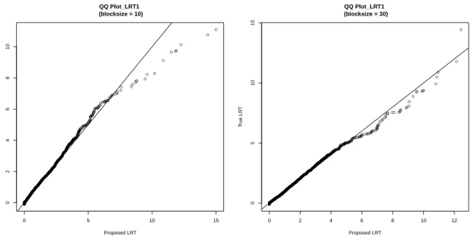
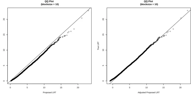
3.1 QQ plot between true LRT1 VS proposed LRT1. . . 53 3.2 QQ plot between true LRT∗ VS proposed LRT∗ for the LD

block with size 10. . . 54 3.3 QQ plot between true LRT∗ VS proposed LRT∗ for the LD

block with size 30. . . 55

4.1 QQ plot between true LRT VS permutedLRT for K =30and ρ=0.5 . . 76

(10)

CHAPTER 1

INTRODUCTION

1.1 Genome-wide Association Study (GWAS)

1.1.1 Introduction of GWAS

(11)

Ragoussis [2009] reviewed several high throughput SNP genotyping platforms. Among all available genotyping platforms, two are most popular: Illumina and Affymetrix. Their popularity is dominant in GWAS. As Ragoussis [2009] mentioned in his review paper, among 209 GWAS papers published until November 2008, data of 103 studies was obtained from Affymetrix Genechips and data of 83 studies was from Illumina’s Infinium Beadchips.

1.1.2 Linkage Disequilibrium

Linkage disequilibrium (LD) describes the degree of no-random association between an allele of one SNP and an allele of another SNP in the same region of the genome. LD can arise in a population for many reasons, and the degree of LD is determined by several factors such as recombination rate, mutation, and demographic features. LD plays an important role in association studies, because suppose all markers are independent at the population scale, the association of every SNP with a trait needs to be investigated, which would present a significant challenge, however, due to the existence of LD, multiple variants could be highly correlated, thus only a subset of SNPs needs to be genotyped in association studies [Laird and Lange, 2011, Section 5.4].

Considering two lociA and B, there exist four possible haplotypes in a population,

due to each separation for two alleles (A,a and B,b). There are several measures of

LD, all of which compare the discrepancy between the observed haplotype frequencies and the haplotype frequencies expected under the null assumption of independence between the two markers. Lewontin and Kojima [1960] proposed the linkage disequi-librium coefficient D and Lewontin [1964] proposed a scaled version ofD,D′ whereD

is standardized by its maximum possible value and D′ varies between 0 and 1. D′=0

(12)

LD. Alternatively, the correlation coefficient r2 (elsewhere, _r2 is also denoted by _∆2) was proposed by Hill and Robertson [1968] for the purpose of genetic analysis, which ranges from 0 to 1. High r2 values indicate that the two SNPs carry similar genetic information and an r2 of 1 indicates perfect predictability of one SNP from another SNP, whereas an r2 of 0 indicates the markers are in perfect equilibrium. _D′ and _r2 are currently the two most widely used LD measurements nowadays [Laird and Lange, 2011, Section 5.4].

Bush and Moore [2012] discussed two categories of the association between a genetic polymorphism and a trait, which are direct and indirect association due to the existence of LD. Specifically, direct association indicates the genotpyed SNP itself is the functional (causal) SNP that can affect biological mechanisms underlying a trait and result in its variation. In other circumstances, only tagSNPs are genotyped and serve as surrogates for the causal locus. Due to the presence of LD between tagSNPs and the causal SNP, the indirect association might be detected between one or more of the tagSNPs and the trait. However, the power to detect significant associations is lower with tagSNPs than that with modeling causal SNPs directly.

1.2 Association Mapping

The goal of GWAS is to investigate the association between genetic variants and complex diseases/phenotypes. The response variable in any genetic association study can be quantitative or qualitative (often binary). The association between the complex trait and the genetic variant can be measured or tested through regression models. The standard method is individual SNP analysis where the effect of each SNP on a trait is examined separately and independently. A list of candidate loci can be selected based on theirp−values less than a given threshold after multiple testing correction [Kraft and

(13)

regression or contingency table is used for a binary trait. For complex diseases, such as obesity and asthma, affection status is often defined by an intermediate phenotype or endpoint phenotype, such as body mass index for obesity or forced expiratory volume in one second (FEV1)for asthma [Laird and Lange, 2011, Section 7.8]. Compared to qualitative traits, association studies with a quantitative measurement as the response variable can be more reproducible, have greater power to detect genetic effects evidence, and offer better interpretations [Bush and Moore, 2012]. In addition to genetic variants, other non-genetic factors such as age or gender are also available to be adjusted for in the statistical model. For a single locus, based on modes of inheritance, genetic models can be divided into four categories: additive, recessive, dominant and multiplicative [Lewis, 2002]. Although the true genetic model is rarely known in practice, signals from both additive and dominant genetic effects can be identified with fairly good power in GWAS using additive models, thus additive models are the most popular models for GWAS data [Bush and Moore, 2012; Lettre et al., 2007].

1.2.1 Methods for Qualitative Traits

In a standard case-control GWAS, a large number of SNPs are genotyped among thousands of individuals with diseases and also for thousands of healthy individuals. The aim is to identify an initial collection of promising susceptibility loci. The frequen-cies of SNP alleles are compared between the case and control groups. Suppose at a given gene, the SNP has two allelesg and Gwith three possible genotypes gg,Gg and GGon a set of cases and controls, the observed frequencies can be summarized in the

following 2×3 contingency table of Table 1.1 [Laird and Lange, 2011, Section 7.1].

(14)

Table 1.1: An example of 2×3 contingency table of genotypes in case-control studies

gg Gg GG Total Cases n11 n12 n13 n1.

Controls n21 n22 n23 n2.

Total n.1 n.2 n.3 n

as [Pearson, 1909, 1910]:

χ2= ∑

i

∑

j

(O_ij−E_ij)2

Eij

,

whereOij is the observed frequency of the genotype in each cell andEij is the expected

value under the null hypothesis. The test statistic approximately follows χ2_{2. If the} sample size is small or an expected cell count is less than 5, then the asymptotic approximation of the null distribution χ2 is no longer valid. Fisher’s exact test is used to calculate the significance of the deviation from the null hypothesis exactly, via a hypergeometric distribution [Tomlinson et al., 2007]. Baz et al. [2008] conducted a case-control study in a Turkish population and used the χ2

2 test to determine if the polymorphisms T N F −α and acne are significantly associated.

For the above test, no prior genetic information is used. However, if prior in-formation is available or a supposition exists that a greater number of allele G will

(15)

identify late-onset Alzheimer disease risk loci in a study using 492 cases and 498 con-trols. By Cochran-Armitage trend test, the 12q13 locus was detected to be significantly associated with late-onset Alzheimer’s disease.

Logistic regression is an alternative way to evaluate genetic associations for di-chotomized disease phenotypes. In addition to genetic variants, many environmental factors could contribute to variations of complex traits, such as age, gender and other demographic characteristics. Inclusion of covariates can dramatically remove their con-founding effects and may improve power. Pirinen et al. [2012] studied the impact of including known covariates on the power of detecting the association in case-control studies. The inclusion of the covariates in logistic regression models generally increases power for common traits. Logistic regression can flexibly model the covariates and has become a standard tool in most GWAS packages such as PLINK by Purcell et al. [2007]. Yu et al. [2012] used logistic regressions in PLINK to perform a two-stage lgA nephropathy (lgAN) study in Han Chinese and identified genome-wide associations at 17q13 and 8p23.

1.2.2 Methods for Quantitative Traits

Quantitative measures better characterize some complex traits, such as high blood pressure, obesity and asthma. For single SNP analysis, Analysis of Variance (ANOVA) is popular. The null hypothesis is that the mean values of a phentoype are the same among all genotype groups. Linear regression is another popular approach for analyzing quantitative traits among n independent samples,

(16)

where for theithindividual,Yiis the quantitative trait,Xirepresents the genetic variant

and Bi is a vector of other covariates to be adjusted for. The advantages of applying

linear regression in GWAS include easy incorporation of covariates under the explicit parametric model and convenient conduction of hypothesis testing through likelihood ratio or score test [Laird and Lange, 2011, section 7.7]. Li et al. [2007] scanned a genome consisting of362,129SNPs among4,305Sardinian individuals and reported that SNPs

in GLUT9 are associated with Uric Acid (UA), by applying a linear regression model. Loos et al. [2008] performed data analysis for genom-wide association data from16,876

subjects using a linear regression model to identify the common variants affecting body mass index.

1.3 Expression Quantitative Trait Loci (eQTL)

(17)

(genomic regions play regulatory roles for different transcripts), classification of clini-cal phenotypes into a cluster of subcategories depending on the cliniclini-cal characteristics and determination of lists of candidate genes based on the knowledge from GWAS for complex diseases [see reviews of Kendziorski and Wang, 2006; Wright et al., 2012].

Various analyses have become well established. Simple linear regression is one of the most commonly used models for eQTL analysis. With millions of SNPs and thousands of transcripts among thousands of individuals in modern eQTL data, eQTL analysis is extremely computationally intensive. Shabalin [2012] proposed Matrix eQTL as a tool for more computational efficient eQTL analysis as follows:

g=α+βs+γx+, i.i.d.∼ N(0, σ2),

whereg is the gene expression,sis the SNP genotype andxrepresents other covariates.

Shabalin [2012] leveraged orthogonalization techniques for the gene expression and SNP with respect to other covariates so that the multiple linear regression model was simplified to a simple linear regression model. Within the simple model framework, test statistics, including t, F and LRT for the null hypothesis H0 ∶β=0, are functions

of the sample correlationr=cor(g, s). For example,t= √

n−2√r

1−r2. The friendly used software, such as Genevar [Yang et al., 2010] and eQTL viewer [Zou et al., 2007], is available for eQTL analysis, output visualization and association results interpretation.

1.4 Multiple Testing Correction

(18)

2005], since it assumes all the tests are independent from each other [Sidak, 1967]. However, neighboring SNPs on a chromosome are likely to be highly correlated due to the presence of the LD and incline to be inherited together (International HapMap Consortium). Another correction method is permutation; it has been widely used in GWAS [Dudbridge, 2006; Tenesa et al., 2008]. One advantage of this method is that the correlation among SNPs is preserved and thus it is less conservative than the Bonferroni correction. However, a permutation procedure can be computationally intensive for large association studies. Zou et al. [2004] proposed an efficient resampling algorithm to determine significance threshold with overall type I error control based on a score test statistic, expressed by a sum of independent random vectors; each vector represents the contribution from one subject to the test statistic. The score test statistic only requires the calculation of estimates under the null hypothesis. Zou et al. [2004] established a detailed derivation of the score test statistic for mapping quantitative trait loci. A multiple linear regression model is considered to test the association between a single SNP and a quantitative trait with inclusion of other non-genetic covariates:

yi=βg_i+γx_i+_i, i=1,⋯, n,

whereyi is the phenotype of theith individual,β is the genetic effect,γ= (γ₀, γ₂, ..., γ_q)

is a vector of coefficients for the intercept and non-gene covariates xi = (1, xi1, ..., xiq).

The log-likelihood of θ= (β, γ, σ2) takes the form

l(θ) =

n

∑

i=1

li(θ),

where li = −1₂logσ2−(yi−βgi−xiγ)

2

2σ2 . In general, we test the null hypothesis H0 ∶ β =0 in

presence of the nuisance parameter vector η= (γ, σ2).

(19)

∂li(β,η)

∂η . The restricted MLEη˜is obtained by solving∑ n

i=1Uη,i(θ) =0underβ =0. η˜, the

estimate of η, does not change from SNP to SNP, and thus only needs to be estimated

once for each transcript in the case that multiple SNPs are examined for one transcript in eQTL analysis. Denote U = ∑n_i₌₁Uβ,i(0,η˜) as the score function for β. The Taylor

expansion and law of large numbers show the equivalence of asymptotic distribution between n−1/2_U and _n−1/2

∑n_i₌₁Ui, where

Ui=Uβ,i(0, η) −Σβ,η(0, η)Ση,η(0, η)−1Uη,i(0, η)

and Σβ,η(β, η) is lim_n_→∞n−1∑n_i₌₁ ∂

2_l

i

∂β∂η and Ση,η(β, η) is limn→∞n−1∑

n

i=1 ∂

2_l

i

∂η∂η [Cox and

Hinkley, 1974, Section 9.3]. The Uis for i=1, ..., n are independent random variables

with mean zero. Zou et al. [2004] claimed thatn−1/2_U is a zero-mean Gaussian process with variance Ξ, which is limn→∞n−1∑n_i₌₁UiUi′. Substituting all unknown parameters

by their sample estimator leads to

ˆ

Ui =U_β,i(0,η˜) −Σ_β,η(0,η˜)Σ_η,η(0,η˜)−1U_η,i(0,η˜).

The consistency of MLE with the law of large numbers indicates that n−1

∑n_i₌₁UiˆUiˆ

′

could be used to estimate Ξ. Denote Uˆ = ∑n_i₌₁Uî and Vˆ = ∑n_i₌₁UîUî

′

, the score test statistic for H0∶β =0 is

W =Uˆ′Vˆ−1U .ˆ

For a single SNP analysis in GWAS, gi represents the genotype score of one SNP in

the additive model. ThenUi is a scalar rather than a vector, thus the expression of the

score test statistic reduces to

W =(∑

n i=1Ui)2 ∑n_i₌₁Ui2

,

(20)

is large.

In contrast to a permutation test, the resampling method only needs to maximize the likelihood of the observed data once, then the significance threshold can be determined. Thus it is computationally less demanding. Alternatively, Diao and Vidyashankar [2013] proposed a modified resampling approach, where the standard normal distribu-tion was replaced by a Rademacher distribudistribu-tion, that is, the random variable takes 1

or−1with equal probability.

The resampling procedure proposed by Zou et al. [2004] is as follows:

1. SimulateGi independently fromN(0,1)(Diao and Vidyashankar [2013] generated

Gi from a Rademacher distribution, whereGi takes the value 1 or -1 with equal

probability).

2. Let U∗(d) = ∑iUˆi(d)G_i and W∗ =U∗(d)T(Vˆ(d))−1U∗(d), then set T∗ to be the

maximum value of W∗(d)for all possible locations d.

3. Repeat the above steps N times whereN is a large integer.

4. Compute the 100(1−α)th percentile of (T₁∗,⋯, T_N∗) as the threshold for a given

significance levelα.

Heredis the SNP location when multiple markers are tested. This resampling method

preserves the correlation structure among multiple score test statistics via the standard normal random variableGi.

(21)

1.5 Twin Studies

Subjects in genetic association studies may be unrelated, or from one family with high correlations such as twin studies. A twin study is a very different study design from a traditional association study, thus a specialized model is needed to account for correlations between twin pairs. Twin studies are commonly used to investigate the associations between genetic variants and complex traits [Chou et al., 2009; Park et al., 2012; Vaccarino et al., 2008]. Typical twin data includes monozygotic twins (MZ) and dizygotic twins (DZ), plus some singletons. MZ twins carry identical genetic informa-tion and are more similar than DZ twins who only share around 50% of their genes

on average. Given that MZ and DZ twins grow in the same environment, the presence of a higher phenotypic correlation indicates that the phenotype is more genetically re-lated between MZ twins than between DZ. Twin studies are often helpful to estimate the heritability by evaluating the contribution from genetic factors to the variation of a complex trait [Boomsma et al., 2002; Neale and Cardon, 1992; Silventoinen et al., 2003; True et al., 1993]. Unlike studies with independent samples, twin studies require more careful statistical modeling techniques, since neglecting genetic relatedness and shared environments among twins may result in high false positive findings.

One popular method is mixed effects models, which have been widely applied to analyze twin and family data with correlation considerations [Carlin et al., 2005; Kuna et al., 2012; Wang et al., 2011]. Another commonly used approach for twin data analysis is structural equation modeling (SEM) [Neale et al., 1989]. SEM is used to measure the contribution from genetic factors to a trait by partitioning the total variation of a trait nto four components. Specifically, Neale et al. [1989] decomposed the total variation of a phenotype into additive genetic effects (ai), dominant genetic effect (di), common

environment effect (ci) and random noise (ei), where ai, ci, di and ei are independent

(22)

N(0, σ2_d), N(0, σ_c2)and N(0, σ_e2) respectively. The genetic model can be written as

yi =µ+g_iβ+x_iγ+a_i+c_i+d_i+e_i, i=1,⋯, n,

where for theith individual,yi is the trait of interest,µis the grand mean,girepresents

genetic variants, and xi denotes covariates. Referring to Falconer and Mackay [1996],

the covariances from the additive genetic effects cov(a_i, a_j) for M Z pairs and DZ

pairs are σ2

a and σa2/2 respectively; the covariances from dominance genetic effects cov(d_i, d_j) for M Z pairs and DZ pairs areσ_d2 and σ_d2/4 respectively; the covariance of

common environmental effect for any twin pairs iscov(c_i, c_j) =σ_c2; the covariances from

additive, dominant and common environment effects are zero for any pair of unrelated individuals. The above model is referred as the ACDE model, however, if parental data are not available, not all random effects can be estimated due to an identifiability issue, in which situation the ACE model is generally used where σ2

d = 0 [Feng et al., 2009;

Wang et al., 2011]. The covariance structures for any pair ofM Z twins,DZ twins and

unrelated singletons are listed as follows,

cov

⎛

⎜ ⎜

⎝

ai

aj

⎞

⎟ ⎟

⎠

= σ2_a ⎛

⎜ ⎜

⎝

1 ρa

ij

ρa

ij 1

⎞

⎟ ⎟

⎠

,

cov

⎛

⎜ ⎜

⎝

di

dj

⎞

⎟ ⎟

⎠

= σ2_d ⎛

⎜ ⎜

⎝

1 ρd

ij

ρd

ij 1

⎞

⎟ ⎟

⎠

,

cov

⎛

⎜ ⎜

⎝

ci

cj

⎞

⎟ ⎟

⎠

= σ2_c ⎛

⎜ ⎜

⎝

1 ρc

ij

ρc

ij 1

⎞

⎟ ⎟

⎠

(23)

where

ρa

ij =

⎧ ⎪ ⎪ ⎪ ⎪ ⎪ ⎪ ⎪ ⎪ ⎪ ⎪ ⎨ ⎪ ⎪ ⎪ ⎪ ⎪ ⎪ ⎪ ⎪ ⎪ ⎪ ⎩

1, if i and j are MZ pairs 1/2, if i and j are DZ pairs

0, if i and j are unrelated

ρd

ij =

⎧ ⎪ ⎪ ⎪ ⎪ ⎪ ⎪ ⎪ ⎪ ⎪ ⎪ ⎨ ⎪ ⎪ ⎪ ⎪ ⎪ ⎪ ⎪ ⎪ ⎪ ⎪ ⎩

1, if i and j are MZ pairs 1/4, if i and j are DZ pairs

0, if i and j are unrelated

ρc

ij =

⎧ ⎪ ⎪ ⎪ ⎪ ⎪ ⎨ ⎪ ⎪ ⎪ ⎪ ⎪ ⎩

1, if i and j are MZ or DZ pairs 0, if i and j are unrelated.

1.6 SNP-set Analysis in GWAS

(24)

one test unit in association studies could enhance the power to identify causal effect with the trait [Schaid et al., 2002]. Moreover, SNP set analyses decrease the number of tests dramatically and thus relieve the stringent significance threshold. Furthermore, if there is more than one independent causal SNPs, their joint activities can be detected with considerable power by performing SNP-set analysis [Wu et al., 2010].

(25)

then the relevant variance components are tested to determine the joint effect of each SNP-set on the complex trait.

A linear mixed model with one variance component can be expressed as follows

Y =Xβ+Zb+ε, E

⎛

⎜ ⎜

⎝

b

ε

⎞

⎟ ⎟

⎠ =

⎛

⎜ ⎜

⎝

0K

0n

⎞

⎟ ⎟

⎠

, cov

⎛

⎜ ⎜

⎝

b

ε

⎞

⎟ ⎟

⎠ =

⎛

⎜ ⎜

⎝

σ2

bΣ 0

0n σεIn

⎞

⎟ ⎟

⎠

,

whereY is an-dimensional response vector, βp×1 is a vector of parameters correspond-ing to fixed effects, K is the number of SNPs in the set, bK×1 is a vector of random effects from individual genetic effects, ΣK_×K is a known symmetric positive definite

matrix, b and are independently and normally distributed. If Y is a trait vector and Z is a n×K matrix used to quantify genetic similarity, then testing forH₀ ∶σ_b2 =0 vs

H1 ∶σ_b2≥0can help determine if SNP-set similarity is significantly associated with trait

similarity. The null distribution ofLRT does not follow the standard 50:50 mixture of

χ2

0 andχ21 in the setting where the genetic effects of all individuals are not independent [Crainiceanu and Ruppert, 2004]. The 50∶50 ratio holds only if the response variable

can be written as a vector including a great deal of independent random variables iden-tically distributed under both the null and alternative hypotheses [Self and Liang, 1987; Stram and Lee, 1994]. This i.i.d. assumption is not true for SNP-set analysis using the model above where the design matrix of random effectsZ cannot be written in the

form of a block diagonal matrix due to the dependency of genetic effects from multiple SNPs among subjects, that is, the response vector cannot be represented as a collection of independent random variables under the alternative hypothesis [Tzeng and Zhang, 2007]. If this i.i.d. assumption is violated, Pinheiro and Bates [2000] in a simulation study found that 0.65χ2

0+0.35χ21 mixture properly approximates the null distribution

(26)

from the variance component method for haplotype-based similarity association anal-ysis comes about because the standard50∶50ratio was used. Crainiceanu et al. [2003]

investigated the null distribution of theLRT statistic and proved that the mixing

pro-portion of χ2

0 can be much larger than 0.5, thus the significance threshold determined by 0.5χ2

0 +0.5χ21 is too conservative for hypothesis testing. Crainiceanu and Ruppert [2004] relaxed the i.i.d. data assumption and developed an efficient resampling proce-dure based on the spectral decomposition of LRT statistic to derive the finite sample

null distribution of the LRT statistic, which only depends on the eigenvalues from two

low dimensional design matrices.

(27)

outcome on both SNP-set and gene expression with their interactions after adjusting for other covariates, then a multiple linear regression model was leveraged to model the relationship between the continuous gene expression and the set of SNPs. The testing procedure for the total effect of a gene from both SNPs and the gene expression was conducted within a causal mediation analysis framework.

1.7 Outline of Thesis

The thesis starts with the literature reviews in the first chapter and the remaining parts are organized as follows. In Chapter 2, we develop a novel and computationally efficient score test statistic to perform eQTL analysis for twin data. In Chapter 3, we investigate a spectral decomposition ofLRT and resampling algorithm to approximate

the null distribution of LRT, which is used to test the association between a set of

SNPs and a phenotype. We propose a modified version of the resampling procedure to approximate the null distribution of LRT for testing the joint effects of SNP-set and

(28)

CHAPTER 2

A FAST EQTL ANALYSIS FOR TWIN STUDIES

2.1 Introduction

(29)

and determination of lists of candidate genes based on the knowledge from GWAS for complex diseases [see the reviews of Kendziorski and Wang, 2006 and Wright et al., 2012]. Recent research has also shown that SNPs detected by GWAS are significantly more likely to be eQTL, which can be used to boost the discovery of genetic variants associated with the trait, and improve understanding of the molecular mechanism of complex traits [Min et al., 2011; Nica et al., 2010; Nicolae et al., 2010].

(30)

realized by a quick matrix operation.

For complex psychiatric disorders, such as schizophrenia and major depressive dis-order, twin studies have received attention for establishing the general extent to which genes and environment are etiologically important [Boomsma et al., 2002; Chou et al., 2009; Neale and Cardon, 1992; Park et al., 2012; Silventoinen et al., 2003; Vaccarino et al., 2008]. Typical twin data include both monozygotic twins (MZ) and dizygotic twins (DZ), plus unpaired individual twins (singletons). MZ twins are assumed to be genetically identical, while DZ twins share 50% of their genes on average. Assuming

that MZ and DZ twins share the same environment, a higher phenotypic similarity between MZ twins compared to DZ twins indicates that the phenotype is genetically controlled. Unlike data with independent samples, twin data require more careful sta-tistical modeling since ignoring genetic relatedness and shared environment among twin pairs may lead to high false and/or low true positive findings. Several statistical ap-proaches are available for twin data. One of the most common apap-proaches is structural equation modeling (SEM) Neale et al. [1989]. Several software programs to perform SEM are available, such as Mx [Neale et al., 1999], Mplus [Muthen and Muthen, 1998], LISREL [Jorsekog and Sorborn, 1986] and OpenMx [Boker et al., 2011, 2012]. Another popular alternative for twin and family data is the mixed-effects model where random effects are used to properly account for the correlations among subjects [Carlin et al., 2005; Kuna et al., 2012; Wang et al., 2011]. Mixed model have a well-established theory which is familiar to statisticians. Moreover, it is conveniently implemented in most sta-tistical software and can flexibly adjust other non-genetic and genetic covariates [Feng et al., 2009; Rabe-Hesketh et al., 2008].

(31)

between twin pairs. To overcome these computational challenges, we propose a novel fast twin eQTL analysis approach. In this approach, we first randomly split the twin pairs into two groups such that within each group, the samples are unrelated. We then run a separate analysis for each group using any statistical procedure valid for indepen-dent data, such as multiple linear regression or analysis of variance. When combining the results from the two groups, we find traditional meta-analysis procedures, such as Fisher’s test, is no longer applicable since the two sets of results are not independent due to the correlation between twin pairs. Naively combining the two sets of p-values without consideration of the dependence structure of the data would lead to inflated false positive findings. In this paper, we propose a novel score test which automatically adjusts the (hidden) correlation structures between twin pairs, and therefore controls the type I error accurately. To demonstrate the computational advantages and evalu-ate the performance of the proposed method, we conduct extensive simulations under various settings to mimic real world twin data.

Our simulation results establish that our proposed approach controls type I er-ror rates well, with negligible power loss compared to the gold mixed effects model. Furthermore, the computational efficiency of the proposed method is dramatically im-proved. The proposed method is more than a thousand times faster than the mixed effects model. The fast performance of the proposed method is achieved by computing the most computationally intensive part in the score test by matrix operations, similar to what has been done in matrix eQTL. The utility of the proposed method is further illustrated by analyzing a twin eQTL data where the twin samples (∼ 4,000) are from

(32)

2.2 Methods

The first step of the proposed approach is to randomly split each twin pair into two groups such that all samples within each group are unrelated. Thus a statistical procedure valid for independent data can be directly applied to each group for testing SNP-transcript pair associations. For simplicity and because of its popularity for eQTL data, multiple linear regression is considered. Specifically, for each group, given a transcript and a SNP, we fit the following linear regression model:

yi=βg_i+x_iγ+_i, i=1,⋯, n,

where for the ith individual, yi is the gene expression, gi is the SNP genotype which

is coded 0, 1 or 2 according to the number of minor alleles in the genotype; and

γ= (γ₀,γ₁, ...,γ_q)

′

is a vector of parameters corresponding to the vector of non-genetic covariates plus the intercept xi = (1, x_i₁, ..., x_iq). Rewriting the above model in matrix

form, we get

Y =βG+Xγ+,

where Y = (y₁, y₂, ..., y_n)′, G= (g₁, g₂, ..., g_n)′ and X = (x′₁,⋯,x′_n)′. The log-likelihood

function is therefore

l(θ) =

n

∑

i=1

li(θ)

where θ = (β,γ, σ2) and l_i = −1₂logσ2−(yi−βgi−xiγ)

2

2σ2 . For the eQTL analysis, the null hypothesis is H0 ∶ β = 0 where the vector of the nuisance parameters is η = (γ, σ2).

Following the derivation procedure of Zou et al. [2004], we get the score function of the

ith individual as

(33)

whereUβ,i(β,η) and Uη,i(β,η) are defined as

Uβ,i(β,η) = ∂li_∂β(β,η) = (yi−βgi_σ−2xiγ)gi,

Uη,i(β,η) = ∂li_∂(β,_ηη) =

⎛

⎜ ⎜

⎝

(yi−βgi−xiγ)x′i

σ2 (yi−βgi−xiγ)2

2σ4 − 1 2σ2

⎞

⎟ ⎟

⎠

, respectively,

and Σβ,η(β,η) is the limit of n−1∑n_i₌₁ ∂

2_l

i

∂β∂η, and Ση,η(β,η) is the limit of n−1∑

n i=1

∂2_l

i

∂η∂η asn→ ∞. The two Hessian matrices are

∂2_l₍_β,_η₎

∂β∂η = ∑

n i=1(−

gizi

σ2 ,−(

yi−βgi−xiγ)gi

σ4 )and

∂2l(β,η)

∂η∂η = ∑

n i=1

⎛

⎜ ⎜

⎝

−x

′ ixi

σ2 −

(yi−βgi−xiγ)x′i

σ4

−(yi−βgi−xiγ)x

′ i

σ4

1 2σ4 −(

yi−βgi−xiγ)2

σ6

⎞

⎟ ⎟

⎠

.

Let the restricted MLE ηˆ be the solution of ∑_i₌₁Uη,i(β,η) =0, where β is set to 0 in

this equation. Specifically, we have

ˆ

γ = (X′X)−1X′Y,

ˆ

σ2 ₌

∑n_i₌₁(y_i−x_iγˆ)2/n= ∣∣Y −Xγˆ∣∣2/n.

Note that ηˆ is estimated under H0 and thus does not depend on the genotypes of any given SNP. Therefore it does not change from SNP to SNP, and needs only to be estimated once for each transcript. Also note that all of the off diagonal elements in ∂2l(β,η)

∂η∂η ∣β=0,η=ηˆ equal to zero. Substituting all unknown parameters by their sample estimators in the score function, we get

ˆ

Ui = U_β,i(0,ηˆ) −Σ_β,_η(0,ηˆ)Σ_η_,_η(0,ηˆ)−1U_η_,i(0,ηˆ)

= (yi−x_ˆiγˆ)gi

σ2 − ∑gixi(∑x

′

ixi)−1(yi−xiγˆ)x

′ i

ˆ

σ2 +

∑ (yi−xiγˆ)gi

nσˆ2 −

∑ (yi−xiγˆ)gi

nσˆ4 (yi−xiγˆ)

(34)

For computational efficiency, we express the score function _Uˆ

i in terms of a matrix

operation below. Denote

a = ∑n_i₌₁gixi=G′X,

A = ∑n_i₌k₁x′_ixi =X′X,

c = ∑ (yi−xiγˆ)gi

nσˆ2 =

1

nσˆ2(G′Y −G′X(X′X)−

1_X′_Y_{) =} 1

nσˆ2G′(I−Mx)Y,

we have

ˆ

Ui=

yi−x_iγˆ

ˆ

σ2 [(gi−aA

−1_x′

i) −c(yi−x_iγˆ)] +c.

Let_Uˆ _{be the vector of the score function of all individuals. That is,}

ˆ

U =

⎛

⎜ ⎜ ⎜ ⎜ ⎜ ⎜ ⎜ ⎜ ⎜

⎝

ˆ

U1

ˆ

U2

⋮

ˆ

Un

⎞

⎟ ⎟ ⎟ ⎟ ⎟ ⎟ ⎟ ⎟ ⎟

⎠ =

⎛

⎜ ⎜ ⎜ ⎜ ⎜ ⎜ ⎜ ⎜ ⎜

⎝

y1−x1γˆ ˆ

σ2

y2−x2γˆ ˆ

σ2

⋮

yn−xnγˆ

ˆ

σ2

⎞

⎟ ⎟ ⎟ ⎟ ⎟ ⎟ ⎟ ⎟ ⎟

⎠ ×

⎡ ⎢ ⎢ ⎢ ⎢ ⎢ ⎢ ⎢ ⎢ ⎢ ⎢ ⎢ ⎢ ⎢ ⎣ ⎛

⎜ ⎜ ⎜ ⎜ ⎜ ⎜ ⎜ ⎜ ⎜

⎝

g1−x₁A′−1a′

g2−x₂A′−1a′

⋮

gn−x_nA′−1a′

⎞

⎟ ⎟ ⎟ ⎟ ⎟ ⎟ ⎟ ⎟ ⎟

⎠ −c

⎛

⎜ ⎜ ⎜ ⎜ ⎜ ⎜ ⎜ ⎜ ⎜

⎝

y1−x₁γˆ

y2−x₂γˆ

⋮

yn−x_nγˆ

⎞

⎟ ⎟ ⎟ ⎟ ⎟ ⎟ ⎟ ⎟ ⎟

⎠ ⎤ ⎥ ⎥ ⎥ ⎥ ⎥ ⎥ ⎥ ⎥ ⎥ ⎥ ⎥ ⎥ ⎥ ⎦

+ ⎛

⎜ ⎜ ⎜ ⎜ ⎜ ⎜ ⎜ ⎜ ⎜

⎝

c

⋮

c

⎞

⎟ ⎟ ⎟ ⎟ ⎟ ⎟ ⎟ ⎟ ⎟

⎠

= (I−M_ˆx)Y

σ2 × [(G−XA′−

1_a′_{) −}_c₍_I₋_M

x)Y)] +J_nc.

Substitutinga, A and c into the above equation, we get

ˆ

U = (I−M_ˆx)Y

σ2 × [(I−Mx)G−

1

nσˆ2(I−Mx)Y Y′(I−Mx)G] +

1

nσˆ2JnY′(I−Mx)G

= {(I−M_ˆx)Y

σ2 × [(I−Mx) −

1

nσˆ2(I−Mx)Y Y′(I−Mx)] +

1

nσˆ2JnY′(I−Mx)}G. (∗)

Note that the elements inside { } only depend on Y and the covariates X, and thus

are the same across all SNPs. This motivates us to derive the above matrix operation to calculate the score vectors across a large number of SNPs for a given transcript simultaneously. Specifically, we replace the vector G in equation (∗) by a matrix

H= (G₁, ..., G_m), whereG_j is theG vector corresponding to SNPj (j =1, ..., m). The

(35)

j. Remember that twin pairs are randomly split into two groups. Notationally let’s

add superscripts to _Uˆ _{above and denote} _Uˆ(1) and _Uˆ(2) as the score matrices of group 1 and group 2, respectively. Also letnk be the number of individuals in the kth group

(k=1,2) and the score function of theith subject for the jth SNP in thekth group be

U_i,j(k) (i=1, ..., n_k), or specifically we now have

ˆ

U(k)=

⎛

⎜ ⎜ ⎜ ⎜ ⎜ ⎜ ⎜ ⎜ ⎜

⎝

ˆ

U₁(_,k₁) Uˆ₁(_,k₂) ⋯ Uˆ₁(_,mk)

ˆ

U₂(_,k₁) Uˆ₂(_,k₂) ⋯ Uˆ₂(_,mk)

⋮ ⋮ ⋯ ⋮

ˆ U_n(k)

k,1

ˆ U_n(k)

k,2 ⋯

ˆ Un(kk),m

⎞

⎟ ⎟ ⎟ ⎟ ⎟ ⎟ ⎟ ⎟ ⎟

⎠

.

The regression results for the jth SNP from the two groups may be naively combined

as

Wnaive(j) =

(∑n_i₌1₁Uˆ_i,j(1))2 ∑n_i₌1₁(Uˆ_i,j(1))2

+

(∑n_i₌2₁Uˆ_i,j(2))2 ∑n_i₌2₁(Uˆ_i,j(2))2

and assumed to follow χ2

2 asymptotically under H0. This test is only valid when the results from the two groups are independent of each other, which is not likely to be true for twin data. To account for the dependence structure of the two groups, we derive a new score statistic to automatically adjust the correlation between the two groups:

Wproposed(j) =

(∑_in₌1₁Uˆ_i,j(1)+ ∑_in₌2₁Uˆ_i,j(2))2

∑_in₌1₁(Uˆ_i,j(1))2+ ∑n_i₌2₁(Uˆ_i,j(2))2+2∑n_i₌twin₁ Uˆ_i,j(1)×Uˆ_i,j(2)

,

where ntwin is the total number of twin pairs, and groups 1 and 2 individuals are

arranged in such way that the first ntwin samples in groups 1 and 2 are paired twins,

and the remaining samples are singletons. The proposed score statistic is assumed to followχ2

(36)

2.3 Simulations and Real Data Analysis

2.3.1 Simulation Studies

The proposed method is applied to simulated twin data to evaluate its performance. Each dataset includes 900 or 1800 individuals consisting of MZ twins, DZ twins and singletons in the ratio 2 ∶2 ∶ 1. Two continuous covariates x_i = (x_i₁, x_i₂) with effects

γ= (0.3,0.1)are correlated to the response variabley_i, wherex_i₁ andx_i₂ are generated

fromN(3,1) and N(5,2), respectively. The response variable y is generated from the

model [Wang et al., 2011],

yi=µ+g_iβ+x_iγ+a_i+c_i+d_i+e_i, i=1,⋯, n,

where for the ith individual, yi is the gene expression, µ is the grand mean, gi is the

SNP genotype, and xi is a vector of non-genetic covariates. The random terms in the

above model ai,di, ci, ei are the additive, dominant, common environment effects and

random error, respectively, which are mutually independent and normally distributed with mean zero and varianceσ2

a, σc2,σd2 and σe2, respectively. For subjects i and j who

are a twin pair, we have cov(a_i, a_j) = σ2_a and cov(d_i, d_j) = σ2_d if they are M Z pair;

cov(a_i, a_j) = σ_a2/2 and cov(d_i, d_j) = σ_d2/4 if they are DZ pair, while cov(c_i, c_j) = σ_c2 for

all twin pairs [Falconer and Mackay, 1996]. According to Neale et al. [1989], the above model is referred to as the ACE or ACDE model depending σ2

d = 0 or not. For each

simulation set up, 1000 datasets are generated. We set σ2

e =1, σ2a=1.5 and σc2 =0.75,

resulting in the additive heritability h2

a of 0.462 and the variance explained by the

shared environmental c2, of 0.231 under the ACE model. For the ACDE model, we setσ2

d to be 1.5, leading to h2a=0.316 and c2 =0.158. Since there are 1000 association

tests for each simulated dataset, 1000 datasets give a total of 1000∗1000 =1 million

(37)

method were compared with three other methods at different significance levels: 1) a multiple linear regression model on the full twin data, where the dependence between the twin pairs is ignored; 2) the naive score approach; and 3) the mixed effects model:

yij =g_ijβ+x_ijγ+a_ij +d_ij+c_ij+_ij, where i and j are family id and individual index

respectively, xij is the vector of non-genetic covariates plus intercept, gij is the SNP

genotype, and the definition ofaij,cij,dij and their covariance structures are described

in the above ACE and ACDE models.

Results from Tables 2.1 and 2.2 demonstrate that the type I error rates of both the proposed method and the mixed effects model are well controlled. In contrast, if the linear regression model (lm) is directly applied to the full twin data, the type I error

rates have been dramatically inflated. For example, under the settings of n=1800 and

the targeted type I error rate α = 0.05, the type I errors for the data from the ACE

model and ACDE model are 0.098 and 0.102, respectively. The type I error inflation in the naive method is also clear.

For power comparisons among the proposed, naive and mixed effect model ap-proaches, we generated1000 datasets under the alternative hypothesis, where we setβ

to0.32,0.37,0.45,and 0.50 in the ACE model andβ to0.40,0.45,0.50,and 0.55in the

ACDE model. For both of the models, the non-genetic effectsγ and the variance

com-ponentsσ2

a,σe2,σc2 and σ2d were kept the same values as those in the above type I error

(38)

Table 2.1: Type I error comparison for data from the ACE model

n=900 n=1800

α 0.05 0.01 0.001 0.0001 0.05 0.01 0.001 0.0001

proposed 0.0522 0.0108 0.0011 0.0001 0.0507 0.0100 0.0010 0.0001 naive 0.0590 0.0159 0.0027 0.0005 0.0577 0.0149 0.0023 0.0004 mixed 0.0509 0.0103 0.0011 0.0001 0.0502 0.0100 0.0010 0.0001 lm 0.0988 0.0301 0.0057 0.0011 0.0984 0.0298 0.0053 0.0010 proposed: proposed score test statistic

naive: naive score test statistic mixed: mixed effects model lm: multiple linear regression

Table 2.2: Type I error comparison for data from the ACDE model

n=900 n=1800

α 0.05 0.01 0.001 0.0001 0.05 0.01 0.001 0.0001

proposed 0.0524 0.0107 0.0011 0.0001 0.0510 0.0104 0.0010 0.0001 naive 0.0604 0.0164 0.0028 0.0005 0.0586 0.0160 0.0027 0.0005 mixed 0.0509 0.0103 0.0010 0.0001 0.0502 0.0101 0.0010 0.0001 lm 0.1024 0.0317 0.0061 0.0012 0.1020 0.0317 0.0061 0.0012 proposed: proposed score test statistic

(39)

Table 2.3: Power comparison for data from the ACE model

β =0.32 β=0.37 β=0.45 β=0.50

Method proposed naive mixed pro naive mixed pro naive mixed pro naive mixed

n=900 α=0.05 0.733 0.721 0.761 0.834 0.834 0.865 0.933 0.934 0.951 0.970 0.964 0.986

0.01 0.503 0.557 0.557 0.664 0.689 0.710 0.830 0.851 0.882 0.899 0.917 0.933 0.001 0.225 0.318 0.286 0.363 0.473 0.434 0.629 0.702 0.696 0.745 0.811 0.811 0.0001 0.103 0.157 0.130 0.166 0.281 0.224 0.368 0.531 0.466 0.530 0.670 0.630

n=1800 α=0.05 0.945 0.944 0.966 0.984 0.982 0.996 1.000 1.000 0.999 1.000 1.000 1.000

0.01 0.831 0.859 0.889 0.940 0.951 0.963 0.989 0.991 0.999 0.999 1.000 0.999 0.001 0.592 0.687 0.690 0.784 0.849 0.867 0.953 0.975 0.983 0.988 0.991 0.999 0.0001 0.344 0.489 0.459 0.567 0.708 0.693 0.864 0.932 0.928 0.951 0.976 0.983 proposed: proposed score test statistic

naive: naive score test statistic mixed: mixed effects model

(40)

Table 2.4: Power comparison for data from the ACDE model

β =0.40 β=0.45 β=0.50 β=0.55

Method proposed naive mixed pro naive mixed pro naive mixed pro naive mixed

n=900 α=0.05 0.740 0.749 0.786 0.842 0.847 0.873 0.904 0.906 0.932 0.949 0.949 0.963

0.01 0.501 0.554 0.561 0.633 0.683 0.688 0.755 0.793 0.804 0.844 0.877 0.890 0.001 0.231 0.298 0.268 0.33 0.433 0.395 0.459 0.576 0.538 0.597 0.694 0.672 0.0001 0.094 0.173 0.122 0.151 0.260 0.201 0.237 0.359 0.299 0.334 0.498 0.426

n=1800 α=0.05 0.964 0.961 0.980 0.986 0.985 0.995 0.995 0.996 0.999 0.999 0.999 0.999

0.01 0.859 0.884 0.913 0.948 0.960 0.971 0.981 0.984 0.990 0.994 0.994 0.998 0.001 0.664 0.740 0.745 0.800 0.858 0.869 0.895 0.944 0.948 0.969 0.981 0.985 0.0001 0.431 0.575 0.511 0.605 0.730 0.703 0.756 0.846 0.844 0.865 0.940 0.927 proposed: proposed score test statistic

naive: naive score test statistic mixed: mixed effects

(41)

2.3.2 Computational Efficiency

Our proposed method combines the advantages of multiple linear regression and the matrix operation to achieve fast computational performance. The proposed method took 361 seconds with one 2.93GHz Intel processor to perform 1 million association

tests whereas the mixed effects model took 21,000 seconds using 100 Intel processors

simultaneously to run the same number of tests. The R function that implements the proposed method can be found atwww.bios.unc.edu/~feizou/software.

2.3.3 Resampling

A common issue in most statistical genetics analysis is the multiple comparison problem. Due to the structure of the genome, test statistics performed at different loci are likely to be correlated, thus Bonferroni correction (which assumes independence of the test statistics) might be too conservative. Permutation procedure [Doerge and Churchill, 1996] is thus widely used for assessing genome-wide significance but the pro-cedure is time consuming. The resampling method for assessing genome-wide statistical significance proposed by Zou et al. [2004] is much more computationally efficient than the permutation procedure, because it only requires to maximize the likelihood of the observed data once. Other advantages of this resampling procedure over the permuta-tion procedure include the flexibility to adjust non-genetic covariates and being more robust to the violation of normality assumption for the data. In our simulation, we bor-rowed the idea from this resampling procedure and modified the proposed test statistic as follows :

W_proposed∗ (j) =

∑_in₌1₁Uˆ_i,j(1)Gi+ ∑_in₌2₁Uˆ_i,j(2)G′_i

(42)

whereGi (i=1,...,n) were generated from i.i.d. standard normal distribution. Diao and

Vidyashankar [2013] generated their Gi from the Rademacher distribution, where Gi

takes value 1 or −1 with equal probability. For each of the two possible distributions

of Gi, we performed resampling 10000 times and calculated their type I error rates

under different significance levels. The results show that the type I error rates are well controlled, which are 0.0526(0.0523) and 0.01147(0.0109) under the significance level

α = 0.05 and 0.01 respectively for Rademacher (standard normal) distribution. The

power is almost the same, with only a slightly increase, as those from the proposed method Wproposed. Table 2.5 summarizes the detailed power comparisons based on the

(43)

Table 2.5: Resampling method power comparison for data generated from the ACE model with different sampling distributions

Rademacher Distribution Standard Normal Distribution

β =0.32 β=0.37 β=0.45 β =0.50 β=0.32 β=0.37 β=0.45 β =0.50

α=0.05 0.734 0.834 0.933 0.970 0.733 0.834 0.933 0.969

0.01 0.509 0.671 0.833 0.903 0.503 0.664 0.830 0.899

0.001 0.242 0.383 0.644 0.760 0.229 0.374 0.632 0.745

(44)

2.3.4 Netherlands Twin Registry (NTR) eQTL Study

A total of 2,752 individuals from the Netherlands Twin Registry (NTR) had their

SNP genotypes and gene expression data measured [Wright et al., 2014] on Affymetrix 6.0 SNP arrays and U219 expression arrays. The goals of this project include quantify-ing the heritability of each transcript and buildquantify-ing a detailed list of eQTL in peripheral blood. After quality control [see Wright et al., 2014, for details], 686,895 SNPs and 47,585 transcripts on 2,494 individuals were used for the eQTL analysis. The 2,494

individuals include 638 MZ pairs, 529 DZ pairs and 160 singletons. A total of 96 co-variates are included in the eQTL analysis, for example, plate number, hybridization well position, gender,and5principal components (PCs) from the gene expression data,

and 3 PCs derived from the SNP data [see Wright et al., 2014].

In contrast to controlling the family-wise error, controlling the false discovery rate (FDR) is less stringent and handles the dependence between test statistics reason-ably well [Benjamini and Yekutieli, 2001]. Instead of saving the p−values for all the

SNP-transcript pairs, Shabalin [2012] only saved thep−values that pass a pre-specified

significance threshold, on which the Benjamini and Hochberg procedure was applied. Following the procedure of Shabalin [2012], we identified 184,474 and 127,891

SNP-transcript pairs at F DR = 0.01 and F DR = 0.001, respectively, with the proposed

method. In contrast, the naive method identified 225,419 and 136,509 significant

SNP-transcript pairs at F DR =0.01 and F DR = 0.001, which are significantly more

than what have been detected by the proposed method. These additional findings are likely to be false positives, given the fact that the type I error inflation of the naive method. Based on the results from the proposed method, SNP-transcripts pairs with

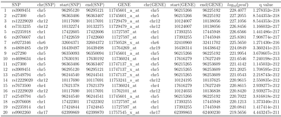
p−values passing certain thresholds are shown in the heat map (Figure 2.1). It clearly

(45)

The top20SNP-transcript pairs detected by the proposed approach are summarized

(46)

Table 2.6: Top 20SNP-transcript pairs identified from the proposed method

SNP chr(SNP) start(SNP) end(SNP) GENE chr(GENE) start(GENE) end(GENE) log10(pval) q value

1 rs3909451 chr5 96295120 96295121 11745601_a_at chr5 96215266 96225192 228.4077 1.278352e-218

2 rs27300 chr5 96363406 96363407 11745601_a_at chr5 96215266 96225192 227.2055 8.544353e-218

3 rs12229020 chr12 10117690 10117691 11729479_a_at chr12 10124007 10138056 227.1056 8.544353e-218

4 rs7313235 chr12 10132274 10132275 11729479_a_at chr12 10124007 10138056 226.8456 1.166032e-217

5 rs2235918 chr1 17422605 17422606 11727597_at chr1 17393255 17445948 226.6566 1.441486e-217

6 rs2076607 chr1 17422659 17422660 11727597_at chr1 17393255 17445948 225.8381 7.908774e-217

7 rs9272346 chr6 32604371 32604372 11750528_x_at chr6 32410960 32411702 225.5650 1.271430e-216

8 rs4808485 chr19 16439497 16439498 11764269_at chr19 16438314 16438642 224.0849 3.360241e-215

9 rs27290 chr5 96350093 96350094 11745601_a_at chr5 96215266 96225192 221.9954 3.670607e-213

10 rs4698634 chr4 17630191 17630192 11736024_at chr4 17616279 17627249 221.6546 7.240198e-213

11 rs27300 chr5 96363406 96363407 11747137_x_at chr5 96215265 96253609 221.4142 1.145032e-212

12 rs3909451 chr5 96295120 96295121 11747137_x_at chr5 96215265 96253609 221.2025 1.708595e-212

13 rs2549794 chr5 96244540 96244541 11747137_x_at chr5 96215265 96253609 221.0543 2.218743e-212

14 rs12229020 chr12 10117690 10117691 11753241_s_at chr12 10124195 10137625 220.9615 2.550835e-212

15 rs7673500 chr4 17621378 17621379 11736024_at chr4 17616279 17627249 220.8615 2.939277e-212

16 rs12229020 chr12 10117690 10117691 11762101_at chr12 10124033 10136838 220.8420 2.939277e-212

17 rs2549794 chr5 96244540 96244541 11745601_a_at chr5 96215266 96225192 220.7022 3.816818e-212

18 rs2076608 chr1 17422301 17422302 11727597_at chr1 17393255 17445948 220.1213 1.373340e-211

19 rs2235914 chr1 17424844 17424845 11727597_at chr1 17393255 17445948 220.0841 1.417414e-211

20 rs9902260 chr17 62399869 62399870 11757545_x_at chr17 62399863 62400230 219.5656 4.443247e-211