FUNDAMENTAL INSIGHTS INTO ELECTRON TRANSFER REACTIONS OF CYCLOMETALATED RUTHENIUM DONOR-BRIDGE-ACCEPTOR COMPOUNDS
Eric J. Piechota
A dissertation submitted to the faculty at the University of North Carolina at Chapel Hill in partial fulfillment of the requirements for the degree of Doctor of Philosophy in the
Department of Chemistry in the College of Arts and Sciences.
Chapel Hill 2019
Electron transfer reactions underlie the whole of chemistry: from C-H bond
formation, to molecular electronics, and in complex proteins found in nature. Accordingly, much of chemistry relies on developing methods to understand and control such reactions to permit the rational design of molecules toward answering contemporary scientific questions. A common approach is the use of model systems which allow theoretical expectations to be tested experimentally. Chapter 1 establishes the framework on which the dissertation is focused through introducing theoretical expectations and predictions for intra- and interfacial electron transfer reactions through a general mathematical and physically intuitive approach. Additionally, the distinction between non-adiabatic and adiabatic reaction mechanisms is made.
This remainder of the Dissertation utilizes model systems of cyclometalated RuII donor-bridge-acceptor compounds to explore mechanisms and pathways through which electron transfer occurs. The donor-bridge-acceptor compounds are covalently linked through a synthetically modifiable aryl-thiophene bridge to an electron-rich triphenylamine unit. Chapter 2 introduces the steady-state spectroscopic, electrochemical, and
spectroelectrochemical characterization of the compounds in fluid solution and anchored onto thin films of TiO2. Further, Chapter 2 quantifies the donor-acceptor electronic coupling
ABSTRACT
Eric J. Piechota: Fundamental insights into electron transfer reactions in cyclometalated ruthenium donor-bridge-acceptor compounds
using UV/Vis/NIR spectroscopy and identifies two pathways through which optical electron transfer can occur, either directly or indirectly.
Chapters 3 and 4 highlight the experimental distinction between adiabatic and non-adiabatic electron transfer using temperature dependent kinetics to determine the rate constant and barriers associated with intramolecular electron transfer. In Chapter 3, the kinetic data indicate that the free energy for the reaction is reduced when the electronic coupling is large. Chapter 4 quantifies the free energies of activation demonstrating that the free energy of activation was independent of reaction (non-)adiabaticity.
Chapters 5 and 6 investigates interfacial electron transfer from either a TiO2 surface or a core/shell SnO2/TiO2 to a molecular acceptor, either the Ru center or triphenylamine unit. Electron transfer from the interface to the triphenylamine unit was found to be bridge independent and indicates that discrete sets of orbitals constitute an electron transfer pathway discussed in Chapter 5. Chapter 6 compares activation energies for interfacial electron
While speaking to Rachel, a fellow lab member, in early January 2019 about our plans for the Spring I said, “It’s going to be hard to thank the many people that have made this…production…possible.” That statement is still true. I’ve been very fortunate to have
many friends, family, and colleagues that have shaped my scientific mindset and personal interests in ways they likely don’t realize. Indeed, everyone I’ve met has contributed in their own important way. Truly there have been many amazing individuals that have impacted my life before and during my graduate work and, at this milestone, it makes sense to take some time to revisit and reflect on the efforts of so many people that ultimately made this
production a reality - if only to have an opportunity to thank them.
This reflection is inspired by an acceptance speech by Mr. Fred Rogers after receiving a Lifetime Achievement Award. In it, he asks the audience, “Would you just take, along with me, ten seconds to think of the people who have helped you become who you are…” and
after the silence concludes, saying, “Whomever you’ve been thinking about, how pleased they must be to know the difference you feel they’ve made…”. It is my sincere hope that the many people who made this possible know that they have made a difference in my life. So if you would, please join me in a brief journey to acknowledge those who I feel have shaped it.
I’d like to begin with my parents, Mary and Frank, and my brother, Greg, for their help throughout my ‘formative’ years. A key aspect in my success now was their limitless
support throughout college career – and their belief in my choice to study Chemistry. The financial help and willingness to be there when they were needed, for rides or advice, made 2010-2014 a amazing time. Their support facilitated my participation in summer programs without needing to worry about working during school or being afraid to chase opportunities. Much of Greg’s (who happens to be a lifelong Carolina basketball fan who recently attended
his first game against Duke in March 2019, Carolina won, 79-70) support stemmed from listening to me attempt to explain nuances of Chemistry, academia, publishing, and electron transfer over the phone or while throwing a football in the backyard during Thanksgiving and Christmas visits. Those conversations helped more than he knows and I hope that I can repay him in a similar way.
Many of my college friends have contributed in ways they likely do not know either. I feel that it is important that I highlight them as well. Their particular contributions have occurred over many years, at different times, and in very different places. So I shall try to be terse. The first group I’d like to highlight are my college ‘roommates’, as they were often the main motivators of my successes, and always happy to support me. The two that stand out are Matthew Libretti and Keighlyn Alber. They instilled in me a feeling of teamwork even though we had different majors, schedules, and interests. I’d like to think we all helped each other equally, but really I was more of a beneficiary of their help than they were of mine. It was their presence during my college career that provided relief and reassurance during many stressful times while at the same time participating in many celebrations, too.
poor way to communicate when yelling was much faster, and that the lines at the Phyrst and Café 210 were not as long as they seemed: Kara Kohler, Michelle Casella, and Kristen Mathious fit this bill. Together, my diverse group of friends made me realize that it is worth balancing social and studious lifestyles.
I’ve had many great teachers, professors, and advisors who I am glad to call friends.
Collectively, they motivated my professional life and validated my choice to study Chemistry in college. In high school, Mrs. Caroline Gold inspired me, a solid ‘B-‘ high school student, to study chemistry through her passion for it. And even though I wasn’t a great student then, she was convinced I could major in chemistry and be successful. At Penn State Hazleton, Dr. Frank Novak was my first advisor who instilled in me an appreciation for Chemistry that I, thinking back, had no business understanding as a freshman. Nevertheless, we would talk almost weekly about electrochemistry and spectroscopy and I distinctly remember reading textbooks light-years above my level of understanding.
mentored me in other important topics like cocktails, movies, and squash (though I could never beat him in a game.) More seriously, it wasn’t until after moving to Chapel Hill that I realized that I had, by chance, independently developed an interest in electron transfer chemistry.
Now I’d like to take the time to thank individual members of Jerry’s research group
over the years (in no particular order): Tim Barr, Brian DiMarco, Evan Beauvilliers, Tyler Motley, Wesley Swords, Matt Brady, Sara Whelin, Erica James, Rachel Bangle, and Michael Turlington, and post-docs Ke Hu, Cassandra Ward, Jenny Schnider, Goucon Li, with a special thanks to Renato Sampaio and Ludovic Troain-Gautier – two inspirational post-docs that I worked closely with. Renato deserves special mentioning as an electron transfer
enthusiast, too. We could waste an entire day discussing it. I’d also like to give special thanks to graduate students in my year: Catherine Burton and Andrew Maurer. Certainly Andrew, more than anyone else, has had to deal with sometimes silly ideas, bad math, and angry rants more than most. I’d also like to give a shout-out to Bruno Aramburu, a visiting student from Argentina, who I had the pleasure of working with for a short three months, and who, at the time of this writing, had just defended his own Dissertation.
In a way everyone I’ve listed contributed either during work or after and the level of friendship in the lab was, and will continue to be, encouraging and often feels like a second family. While I have limited experience in other groups, I feel that the dynamic is unique and powerful. Indeed, over the time I’ve been in this lab, it has always been close nit,
darts at a board while they tackle their on complicated research problems. Teamwork is certainly a strength of the group.
Next, I’d like to thank my advisor, Jerry Meyer, for the last four and a half years of
advice, insight, and attention. His incredible knowledge of the literature, skillset in clear and concise writing, and genuine interest in each of our research projects is inspiring. Even though I‘ve beat Jerry in squash, where he may have learned a move from me. As a testament
to his expertise, I’ve never walked away from a research discussion without learning
something new, either. An impressive feat, in my opinion, is that he managed to deal with me for over four years, let me ‘follow my nose’ in many different electrons transfer projects, and
took interest when I would discuss very niche aspects of electron transfer theory. Maybe I wasn’t the graduate student he expected, but working in his lab has impacted my scientific
interests and focus on a fundamental level. I owe him a debt of gratitude for the last four years, both to him and the many members of the lab, for advising and help in research and my growth as a scientist.
As I’m rapidly approaching the end of my acknowledgements, I owe the largest
weekend in Asheville, and we always made time to relax and laugh together. In this way, she’s contributed not only to my successes in graduate school, but also to my intense interest
in cooking, brunch (a cornerstone of our relationship), and to re-watching The Office. It is challenging to articulate my appreciation for what she’s done for me in just a few sentences, and how she’s helped and shaped by graduate student experience and life as a whole. And so,
Anginelle: Thank you for everything; for all your help and all you do to make our lives function smoothly. I am a very lucky to have you in my life.
LIST OF FIGURES ... xix
LIST OF SCHEMES... xxvi
LIST OF TABLES ... xxvii
Chapter 1. Intramolecular and interfacial electron transfer theory ...1
Motivation ...1
Electron transfer reactions...3
Marcus theory...5
Using potential energy surfaces and Marcus theory to understand electron transfer ...7
1.4.1 Non-adiabatic potential energy surfaces ...7
1.4.2 Gibbs energy of activation...9
1.4.3 Reorganization energy ...10
1.4.4 Electronic coupling ...13
Applications of potential energy surfaces in thermal and optical electron transfer ...18
1.5.3 Arrhenius and Eyring models ...22
Genesis of the Marcus equation ...23
1.6.1 Nuclear factors...23
1.6.2 Electronic and nuclear transmission coefficients ...25
1.6.3 Adiabatic electron transfer ...29
Conclusion ...31
REFERENCES ...32
Chapter 2. Optical intramolecular electron transfer in opposite directions through the same bridge that follows different pathways ...39
2.1 Introduction ...39
Results ...42
Discussion ...49
2.3.1 Electrochemistry ...51
2.3.2 Mulliken-Hush HDA calculations ...53
2.3.3 Superexchange HDA calculations ...57
Conclusions ...60
Experimental methods ...62
2.5.1 Thin films and sensitization...62
2.5.2 Spectroscopic characterization ...63
2.5.4 Surface spectroelectrochemistry ...64
2.5.5 Chemical oxidation ...65
Acknowledgements ...65
Additional content ...66
2.7.1 Chemical oxidation ...66
2.7.2 Accounting for comproportionation ...67
2.7.3 Deconvolution of the mixed-valent spectrum ...70
2.7.4 Reconstructing the mixed-valent spectrum ...71
2.7.5 Result of comproportionation correction and electrochemical modeling ...72
2.7.6 Assignment of the TPA to cyclometalating ligand charge transfer transition ...73
2.7.7 Spectroelectrochemical data of the x-series ...75
2.7.8 Synthesis of the Studied Compounds ...76
REFERENCES ...77
Chapter 3. Kinetics teach that electronic coupling lowers the free energy change that accompanies electron transfer ...85
Introduction ...85
3.1.1 The theoretical prediction that electronic coupling, HDA, lowers Go ...87
3.1.2 The kinetic approach ...88
3.2.2 Application of the kinetic approach ...92
3.2.3 Free energy loss due to electronic coupling ...98
Conclusions ...102
Additional information ...102
3.4.1 Experimental details ...102
3.4.2 Sample preparation ...102
3.4.3 UV-vis absorption ...103
3.4.4 Transient absorption ...103
3.4.5 Electrochemistry ...104
3.4.6 Calculations ...104
3.4.7 Calculation of HDA through the generalized Mulliken-Hush model ...105
3.4.8 Determination of HDA for 1x and 1p ...107
3.4.9 Kinetic model ...109
3.4.10 Derivation of the Gibbs free energy surfaces ...112
3.4.11 The adiabatic double minimum limit ...115
3.4.12 Acknowledgements ...117
REFERENCES ...119
Chapter 4. Entropic barriers determine adiabatic electron transfer equilibrium ...123
Introduction ...123
Discussion ...128
4.3.1 Pre-exponential factors ...129
4.3.2 Entropy of activation ...133
4.3.3 Enthalpy of activation...135
4.3.4 Free energy of activation ...136
4.3.5 A priori rate calculations ...138
4.3.6 Reorganization energy ...140
4.3.7 Standard thermodynamics ...142
4.3.8 Origin of entropic barriers ...143
Conclusions ...146
Additional content ...147
4.5.1 Calculation of the reorganization energy ...147
4.5.2 Temperature dependence of the reorganization energy and adiabaticity factor ...148
4.5.3 Nonadiabatic kinetics ...150
4.5.4 Adiabatic kinetics ...152
4.5.5 Marcus and Eyring model equivalence ...154
Acknowledgements ...158
REFERENCES ...159
Introduction ...165
Results ...168
5.2.1 Spectroscopic and redox properties ...168
5.2.2 Bridge-mediated electronic coupling ...170
5.2.3 Time-resolved absorption spectroscopy ...171
5.2.4 Electron transfer kinetics ...173
Discussion ...174
Conclusions ...177
Additional content and experimental details ...178
5.5.1 Sensitized thin films ...178
5.5.2 Spectroelectrochemistry ...178
5.5.3 Transient absorption spectroscopy ...178
5.5.4 Density functional theory calculations ...179
5.5.5 HDA Calculations ...179
Acknowledgements ...180
REFERENCES ...182
Chapter 6. Barriers for interfacial back-electron transfer: a comparison between TiO2 and SnO2/TiO2 core/shell structures ...186
Introduction ...186
Discussion ...194
6.3.1 The kinetic model: ...195
6.3.2 Models for back-electron transfer ...197
Conclusion ...201
Additional Details ...202
6.5.1 Materials ...202
6.5.2 Preparation of SnO2 and TiO2 colloidal suspensions. ...202
6.5.3 Preparation of TiO2 and SnO2/TiO2 core/shell thin films. ...203
6.5.4 UV−Vis absorption ...204
6.5.5 Transient absorption ...204
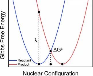
Figure 1.1. Gibbs free energy surfaces of reactants (blue) and products (red) calculated with equations x and y. The nuclear configuration along the abscissa represents the nuclear arrangement (molecule and solvent). The vertical transition from the minimum of the reactant to the product curve is the reorganization energy and the transition state, represented by ΔG‡, is where the product and reactant
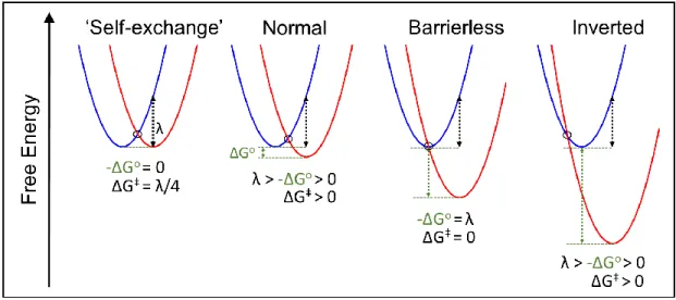
energies are equal. ... 8 Figure 1.2. Four primary types of electron transfer reactions categorized by
relationship between ΔGo and λ, except for self-exchange. ... 10 Figure 1.3. A molecular view of the reorganization energy corresponding to thermal
and optical non-adiabatic electron transfer. (1)-(2): Beginning from the equilibrium configuration of the reactant (blue) absorption of light with ΔGo = h𝜈 = λ generates the electronic configuration of the product (red) in the nuclear configuration of the reactants (Born-Oppenheimer approximation). (1)-(3): Thermal electron transfer over the transition state GTS = ΔG‡ = λ/4 results in formation of the equilibrium
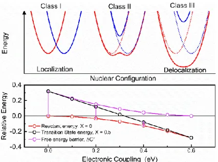
electronic and nuclear configuration of the product. ... 11 Figure 1.4. Effect of electronic coupling on potential energy surfaces as categorized
by Robin and Day. Class I electron transfer (top left) corresponds to HDA = 0, electrons are valence-localized, with a maximum barrier for electron transfer ΔG‡ (bottom left). In class II, HDA > 0, electron density is partially delocalized (top middle), and electron transfer between reactants and products is discrete (and can be adiabatic), while the barrier is reduced ΔG‡ad< ΔG‡ (bottom middle). In class III electron density is delocalized (top right) and electron transfer is not discrete. As a result, there is no barrier for electron transfer, ΔG‡ = 0 (bottom right), as the reactant
minimum energy is equal to the energy of the transition state. ... 17 Figure 1.5. Three schematic representations of interfacial electron transfer. (left) A
molecule, D, is immobilized onto a mesoporous substrate of TiO2. Following light excitation (1) electron transfer to the surface occurs from a localized molecular excited state to form D+ (2) on the timescale of microseconds before the electron recombines with D+ (3). (middle) A D-B-A molecule is immobilized onto a TiO2 surface and, following excitation of D, injects an electron into the surface (2), after which a quasi-equilibrium between D and A may be established on the nanosecond timescale (4) which allows recombination to occur to either D+ (3) or A+ (5). (Right) Immobilization of D-B-A onto a core/shell film of SnO2/TiO2 increases the lifetime of the electron in the surface by virtue of the energy difference of the conduction band energies of SnO2 and TiO2 allowing the quasi-equilibrium to be established (4) before recombination via activated electron transfer (6) or tunneling (7) occurs to
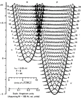
Figure 1.6. Reactant (left) and product (right) potential energy surfaces of Marcus-inverted electron transfer reactions showing vibrational wavefunction sub-levels. Higher energy vibrational energies (n = 7 for reactants) and (n = 16 for products) show how excited-vibrational states facilitate inverted electron transfer. Adapted
from Barbara et. al.53 ... 24 Figure 1.7. (A and B) Nuclear factors for electron transfer reactions. The electron
donor (blue) or acceptor (red) is influenced by inner-sphere-type vibrational Donor-Ligand modes 𝜈i with frequencies between 1012-1013 s-1. Brown ovals (with tan oval backgrounds) show outer-sphere solvent rotational motion, 𝜈o, which are slower than vibrational motion with 𝜈o = 1010-1012 s-1. (C) Electronic factors following from the Golden Rule where electronic coupling, HDA, is represented by orbital overlap from the reactant and product wavefunctions. The electron transfer rate is limited by
𝜈el < 𝜈n when the orbital overlap is weak whereas strong overlap can cause nuclear
motion to be rate limiting, 𝜈n < 𝜈el. ... 27 Figure 1.8. (Top) The electronic transmission coefficient as a function of HDA for
the indicated values of nuclear frequencies, 𝜈n, with λ = 1 eV. (B) The electronic frequency (red dotted line) or the product of 𝜈n and κel as a function of HDA. Red circles indicate the magnitude of electronic coupling necessary to achieve κel = 1,
i.e. adiabatic electron transfer. When the colored lines (brown through green) deviate from 𝜈el (red dotted) electronic coupling becomes sufficiently large for the reaction to become limited by 𝜈n instead of 𝜈el. Values of 𝜈n were chosen to correspond to the timescales shown in the lower figure, from slow rotational motion to delocalized electronic motion. Vertical dotted lines corresponding to HDA = kbT and λ/2 set boundary conditions establishing that coupling brought about by thermal energy fluctuations does not always result in adiabatic electron transfer and that ΔG‡
> 0. ... 28 Figure 2.1. Absorption spectra of the ester forms of the compounds in neat CH3CN
(left). Absorption spectra of the carboxylate forms of the compounds in CH3OH
containing tetrabutylammonium hydroxide (right). ... 43
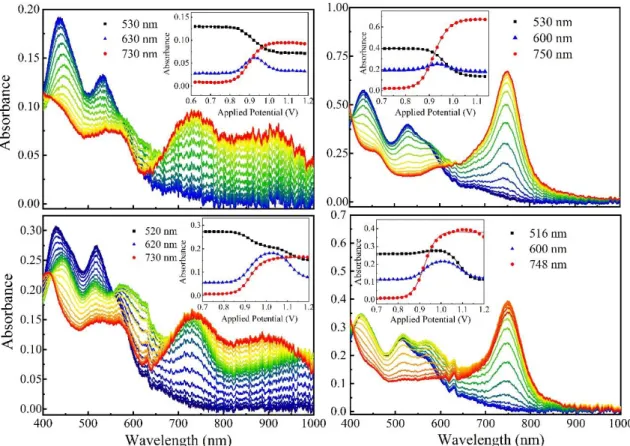
Figure 2.2. Representative spectroelectrochemical data for 1pE (upper left), 2pE
(lower left), 1xE (upper right) and 2xE (lower right) in CH3CN containing 0.1M
LiClO4. Insets show single wavelength absorption changes as a function of applied
potential, and all applied potentials are reported vs. NHE. ... 45
Figure 2.3. Spectroelectrochemical oxidation of 1pC/nITO (left) and 2pC/nITO
(right). Insets show difference spectra taken relative to 0 mV of applied potential.
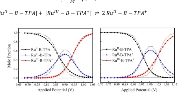
Applied potentials are vs. NHE. ... 46 Figure 2.4. Plots of mole fractions for 1pC/nITO (left) and 2pC/nITO (right) in the
Figure 2.5. Absorption spectra of 1pC/nITO (top) and 2pC/nITO (bottom) in their
ground (black), one-electron oxidized (blue), and two-electron oxidized (red) states. The dashed blue line represents the comproportionation correction in the mixed valent state from spectral modeling which reveals intense IVCT-type transitions at
450 nm for 1pC/nITO and 1100 nm for 2pC/nITO. ... 48
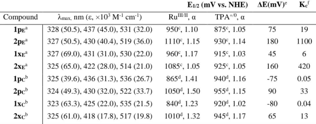
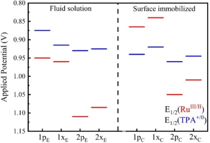
Figure 2.6. Representation of E1/2(RuIII/II) (red) and E1/2(TPA+/0) (blue) for the 8
compounds in fluid acetonitrile solution and immobilized nITO. ... 52 Figure 2.7. Redox potential switch upon surface immobilization for 1pE and
1pC/nITO as well as 1xE and 1xC/nITO. The dashed lines connecting the redox
potentials are guides to the eye. ... 53 Figure 2.8. UV-Vis-NIR absorption spectra of 1pE (left) and 2pE (right) in neat
CH3CN with Cu(II) titrated in as a chemical oxidant. Note the appearance of low
energy IVCT transitions at ~1000 nm for both compounds. ... 56 Figure 2.9. Difference spectra of 1pE (left) and 2pE (right) as a function of added
equivalents of Cu(II). ... 67 Figure 2.10. Plots of mole fractions of each species as a function of added Cu(II)
for 1pE (A) and 2pE (C), and as a function of applied potential for 1pC/nITO (B)
and 2pC/nITO (D). ... 68
Figure 2.11. Measured extinction coefficients after accounting for
comproportionation for 1pE and 2pE (left) and 2pC/nITO (right). ... 70
Figure 2.12. Deconvoluted spectra of 1pE (top left), 1pC/nITO (top right), 2pE
(bottom left), and 2pC/nITO (bottom right). Dashed red lines indicate the
cumulative spectra of all Gaussian bands needed to fit the spectrum adequately. ... 71 Figure 2.13. Comparison of 1pE (left) and 2pE (right) spectra after being corrected
for comproportionation. Note the large difference from similar spectra in the main
text for 1pC/nITO and 2pC/nITO. ... 72
Figure 2.14. Spectra of the free ligands in 0.1M LiClO4/CH3CN. (Left) Ligands containing a methoxy substituent that most closely resemble the 1-series. The green and black lines are ground-state spectra while the red and blue lines are oxidized by one electron. (right) ligands containing a CF3 substituent that mimic the 2-series. The green and black lines are ground-state spectra while the blue and red are
one-electron oxidized. ... 74 Figure 2.15. Comparison of ground-state spectra of 1pL (green) and one-electron
oxidized 1pc/nITO (dashed blue line). ... 75
Figure 2.16. Spectroelectrochemical data of 1xC/nITO (left) and 2xC/nITO (right)
Figure 3.1. The A-B-D compounds utilized. Four cyclometalated ruthenium (blue) compounds with carboxylic acid groups (for binding to TiO2) and an aromatic bridge covalently bound to a triphenylamine unit (red). Methyl substitutents in the R3 positin – xylyl bridge (x) – lowers electronic coupling relative to the phenyl-bridge (p, R3 = H). The R1 and R2 substitutents allow the Eo(RuIII/II) potentials to be
controlled for the 1 and 2 series while Eo(TPA+/0) was held constant. ... 86 Figure 3.2. Potential energy surfaces and kinetic approach. (a), Gibbs free energy
surfaces (GESs) that represent a redox equilibrium between A-B-D (blue) and A- -B-D+ (red) as the electronic coupling matrix element (HDA) is increased from 0 (nonadiabatic) to over 3000 cm-1 (adiabatic). Emphasis is placed herein on the reduction in the Gibbs free energy change, |Go| > |Goad|, that accompanies the transition from non-adiabatic to adiabatic electron transfer in the double minimum regime. (b) A ‘reaction coordinate’ diagram with potential energy surfaces of D-B-A reactants and D+-B-A- products and semiconductor energetics. The kinetic approach used to quantify the thermal electron transfer reaction consists of a RuII -B-TPA compound anchored to the surface of mesoporous thin films of TiO2 (the secondary acceptor). Light absorption induces excited-state electron injection from the RuII unit into the TiO2 to form TiO2(e-)|-RuIII-B-TPA. Within the time frame of charge recombination, the dynamic equilibrium RuIII-B-TPA ⇋ RuII-B-TPA+ was quantified through a kinetic model that afforded the forward, k1, and reverse, k-1,
electron transfer rate constants... 89 Figure 3.3. Electronic properties and transient absorption data. (Upper) The visible
absorption spectra of 2x (a) and 2p (b) anchored to In2O3:Sn thin films. Highlighted in the shaded orange area are the intervalence transition bands. The insets show the molecular structure with the overlaid highest occupied molecular orbitals (HOMO) generated from DFT calculations. (Middle) Absorption difference spectra measured at the indicated delay times after laser excitation for 2x (c) and 2p (d). The insets show normalized single wavelength kinetic data monitored at 700 nm (that reports predominantly on TPA+ concentrations) and at 510 nm (due to RuIII). (Bottom) Single wavelength data that reports on the time dependent TPA+ concentration as a function of temperature for 2x (e) and 2p (f). Overlaid in yellow are fits to the kinetic model used, as described in the Supplementary Information. The insets display Arrhenius plots of the forward, k1, and reverse, k-1, rate constants. All experiments
were performed in 0.1 M LiClO4/acetonitrile solution. ... 94 Figure 3.4. Single wavelength data that reports on the time dependent TPA+
concentration as a function of temperature for 1x (a) and 1p (b). The insets display an Arrhenius plot of the forward, k1 (red), and reverse, k-1 (blue), rate constants. Overlaid in yellow are fits to the kinetic model used, as described in this
Supplementary Information. ... 95 Figure 3.5. van’t Hoff analysis and the influence of electronic coupling on Gibbs
free energy for electron transfer calculated from numerical analysis of the GESs (equation (4)) with the indicated reorganization energies, λ. The solid lines represent the progression of the nonadiabatic Go to the adiabatic value, Goad, limited to the double minimum regime. The dotted lines denote fictitious Goad values for a GES
collapsed to a single minimum. ... 98 Figure 3.6. Chemical oxidation of 1p (left) and 2p (right), in acetonitrile solutions,
using Cu(ClO4)2 as the sacrificial oxidant. ... 109 Figure 3.7. Gibbs free energy surfaces generated from equation 22 for fixed = 0.6
eV and Go = 70 mV with the indicated HDA values. For HDA = 0.1 eV an adiabatic double minimum GES occurs. At HDA = 0.2 eV, the energy minimum of the donor, G(D), equals that of the transition state, G(TS). When HDA values are greater than 0.2 eV, for instance HDA = 0.4 eV, the acceptor and donor GES collapses to a single
minimum. ... 116 Figure 3.8. a) Energy values abstracted for the acceptor and donor minima and the
transition state with fixed = 0.6 eV and Go = 68 mV, with varying HDA. The inset highlights the HDA value at which the acceptor and donor GESs collapses to a single minimum for different values of . b) HDA values (in eV and kT) units necessary to
collapse the GESs into a single minimum for multiple combinations of Go and . ... 117 Figure 4.1 van’t Hoff plot of electron transfer equilibrium constants for the studied
compounds.15 Adapted from Ref. 15. Uncertainty in ln(Keq) is ± 0.05. ... 126 Figure 4.2. Arrhenius (top) and Eyring analysis (bottom) for the forward, TPA →
RuIII, kTPA, (open shapes) and reverse, RuII → TPA+, kRu (solid shapes) electron transfer rate constants for 1x, 1p (red triangles) and 2x, 2p (blue circles). Errors in
the rate constants are ± 5%. ... 128 Figure 4.3 Electron transfer rates as a function of electronic coupling for a purely
non-adiabatic reaction (Eq. 8, κA = 0, black), a non-adiabatic reaction with the adiabaticity parameter (Eq. 8, κA > 0, red) and a solvent-controlled adiabatic reaction (Eq. 10, dashed blue line). Parameters used in these calculations: T = 298 K, λ = 1
eV, τL = 0.2 ps, ΔG‡ = 24 kJ mol-1. ... 139 Figure 4.4. TD-DFT optimized structure of 2p used to determine geometric
distances for estimation of the reorganization energy. ... 148 Figure 5.1. The strategy utilized to demonstrate an electron transfer pathway from
cannot be attributed to distance or driving force and must result from an interfacial
electron transfer pathway that utilizes the bridge orbitals. ... 167 Figure 5.2. The interfacial density of states for 1x/TiO2, 1p/TiO2, 2x/TiO2,2p/TiO2
in 0.5 M LiClO4/CH3CN. The distributions shaded in blue correspond to RuIII/II
redox equilibria and that shaded in red corresponds to TPA+/0. ... 169 Figure 5.3. The spectroscopic evidence for preferential interfacial electron transfer
from TiO2 to the RuIII center through the xylyl bridge. (A) The transient absorption difference spectra measured at the indicated delay times after pulsed 532 nm excitation (0.2 mJ/cm2) of 2x/TiO2 in 0.5 M LiClO4/CH3CN; and (b) the decay
associated spectra (B) that show how the concentrations of RuIII (blue) and of TPA+
(red) change with time. ... 172 Figure 5.4. Comparative kinetic analysis showing that reduction of TPA+ and RuIII
were the same for the phenyl bridge, 𝑘𝑅𝑢𝐼𝐼𝐼/𝑘𝑇𝑃𝐴 + = 1, and were significantly influenced by the xylyl bridge, 𝑘𝑅𝑢𝐼𝐼𝐼/𝑘𝑇𝑃𝐴 + > 10. Single wavelength kinetic data measured after pulsed 532-nm excitation (0.2 mJ/cm2) of A) 2x/TiO2 and B) 1x/TiO2 immersed in 0.5 M LiClO4/CH3CN solution at wavelengths that correspond mainly to recombination to RuIII (blue), monitored at 510 nm, and TPA+ (red) monitored at 750 nm. The insets show recombination data for 2p/TiO2 and 1p/TiO2,
of RuIII and TPA+ monitored at 550 nm and 740 nm, respectively. ... 174 Figure 6.1: Structure of the D-B-A sensitizers bearing either a xylyl bridge (R =
CH3, CF3-x) or a phenyl bridge (R = H, CF3-p) anchored on different metal oxides (TiO2 or SnO2/TiO2 core/shell). The recombination reaction from electrons in the
metal oxides to the oxidized RuIII or the oxidized TPA+ is highlighted. ... 188 Figure 6.2: Absorption spectra of CF3-p and CF3-x recorded in methanol at room
temperature. ... 189 Figure 6.3: Transient absorption difference spectra measured over the indicated
time range after pulsed 532 nm light excitation of TiO2|CF3-p (a), TiO2|CF3-x (b), CS|CF3-p (c) and CS|CF3-x (d) thin films submerged in argon purged 0.1M LiClO4
CH3CN electrolyte. ... 191 Figure 6.4: The absorption change monitored at 730 nm after pulsed 532 nm
excitation of TiO2|CF3-p (a), TiO2|CF3-x (b), CS|CF3-p (c) and CS|CF3-x (d) over the temperature ranges indicated. The dye-sensitized thin films were immersed in
an argon purged 0.1M LiClO4 CH3CN electrolyte solution. ... 192 Figure 6.5: Arrhenius (left) analysis of back-electron transfer at the indicated
dye-sensitized interfaces. The open shapes correspond to back-electron transfer from MOx(e-) to RuIII whereas the solid shapes correspond to back-electron transfer from MOx(e-) to TPA+. A van’t Hoff plot (right) obtained from the intramolecular
Figure 6.6: Representation of two models previously used to rationalize the kinetics for back-electron transfer from SnO2/TiO2 core/shell nanoparticles to oxidized sensitizers or redox mediators. On the left, the conduction band edge band edge potential of TiO2 is represented for illustration purposes as a solid red line. The band edge offset model between SnO2 and TiO2 is represented in the middle while the formation of a low energy SnxTiyO2 electronic state at the interface between the
SnO2 core and the TiO2 shell is represented on the right. ... 197 Figure 6.7: Activation energies for back-electron transfer from TiO2(e-) to oxidized
Scheme 1.1. Three types of electron transfer reactions. ... 4 Scheme 1.2. Nuclear motion through the transition state associated with
(non)adiabatic electron transfer reactions. ... 18 Scheme 2.1. Representation of the reversal of the electron transfer pathway
following one-electron oxidation.a ... 41 Scheme 2.2. Nomenclature and structures of the 8 compounds studied. ... 42 Scheme 2.3. Representation of superexchange theory for bridge-mediated electron
transfer (left) as well as for the ‘indirect’ electron transfer pathway when RuII is oxidized prior to TPA (middle) and the ‘direct’ pathway when TPA is oxidized first
(right). ... 51
Scheme 2.4. Potential energy surface diagram for 3-state optical electron transfer.a ... 54 Scheme 2.5. Previously reported cyclometalated RuII mixed-valent compounds with
the corresponding values of HDA. Taken from ref. 46-48 and 52. ... 57
Scheme 2.6. Structures of the ligands prior to coordination to RuII. ... 73 Scheme 3.1 Square-scheme kinetic model for molecules that undergo excited-state
acid-base chemistry. ... 109 Scheme 3.2. Square-scheme kinetic model for interfacial (kA, kb) and intramolecular
(k1, k-1) electron transfer for immobilized molecules. ... 110 Scheme 4.1. Redox equilibrium after excited state injection to TiO2. ... 124 Scheme 4.2. Two-dimensional potential energy surfaces for asymmetric electron
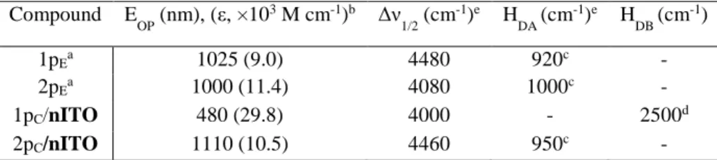
Table 2.1. Spectroscopic and electrochemical properties of the compounds studied.
... 43 Table 2.2. Tabulated values of IVCT band parameters and the associated electronic
coupling matrix elements. ... 56
Table 2.3. Parameters of the IVCT bands used to calculate HDA. ... 71 Table 3.1. Thermodynamic and Electronic Coupling Parameters at Room
Temperature. ... 91 Table 3.2. Arrhenius Parameters Extracted from Temperature Dependent Rate
Constants. ... 96 Table 3.3. Calculated and experimental values for dipole-moments, degree of
delocalization, electron transfer distances, and electronic coupling for the 2p
compound. ... 107 Table 3.4 Rate and Equilibrium Constants from the Kinetic Analysis. ... 111 Table 4.1. Thermodynamic values for the indicated compounds in the redox
equilibrium of Eq. 1. ... 126 Table 4.2. Activation parameters for intramolecular electron transfer in the
xylyl-bridged (nonadiabatic) and phenyl-xylyl-bridged (adiabatic) compounds. ... 128 Table 4.3. Standard and thermodynamic activation entropies for electron transfer. ... 134 Table 4.4. Calculated and observed rate constants of intramolecular electron
transfer at 293 K... 140 Table 4.5. Rate constants for 2x calculated with reorganization energy as a
temperature dependent and independent value. ... 149 Table 4.6. Temperature dependence of the adiabaticity parameter, κA, at λ = 1.15
eV. ... 150 Table 4.7. Experimental and calculated rate constants for electron transfer in the
nonadiabatic limit in compound 1x... 151 Table 4.8. Experimental and calculated rate constants for electron transfer in the
Table 4.9 Experimental and calculated rate constants for electron transfer in the
adiabatic limit in compound 1p. ... 153 Table 4.10. Experimental and calculated rate constants for electron transfer in the
adiabatic limit in compound 2p. ... 153 Table 4.11. Errors for standard thermodynamic quantities from the van’t Hoff
analysis. ... 154 Table 5.1. Reduction Potentialsa and Rate Constants for 1-2/TiO2. ... 170 Table 6.1: Activation parameters for the back-electron transfer reaction from TiO2
Intramolecular and interfacial electron transfer theory Motivation
Studies of electron transfer events within and between molecules has permeated the diverse fields of biology, physics, and chemistry which have captivated the minds of countless scientists over many generations. The ubiquity and fundamental insight provided by studying such reactions lends itself to the diversity of fields that are concerned with electron motion. In the field of Chemistry in particular, electron transfer reactions are studied, intentionally or not, in nearly every one of the sub-disciplines that comprise it and are present in nearly every physical medium. It is worth mentioning sub-disciplines of chemistry that have embraced this fundamental process. Biological chemistry, for example, studies electron transfer reactions between redox-active sites in an enzymes or proteins1-2, or between DNA base-pairs.3-4 Meanwhile, analytical and materials chemists interested in sensors5, microelectrodes6-7, or microscopy techniques8-9 are also concerned with electron transfer. Inorganic and physical chemists are inherently interested in electron transfer
reactions within well-defined transition metal containing bioinorganic,10-14 or organometallic model complexes with time-resolved spectroscopies spanning over 21 orders of magnitude in time15-23, or as theoretical problems studied with quantum theory24-25. Certainly, some
Insofar as physical-inorganic chemists are concerned (where electron transfer is central to the field’s scientific philosophy) an electron transfer ‘puzzle’ is often comprised of 1)
determining the mechanism through which electron transfer occurs, 2) what principles
govern it, and 3) what chemical factors contribute to it. However, like any challenging puzzle there exists extensive, exhaustive, and elaborate theoretical insights into what the best way to ‘solve’ it is. For studying electron transfer reactions the theoretical basis on which the field
has grown (and continues to grow beyond) is that of theory of Libby and Marcus (who was recipient of the 1992 Nobel Prize for his contributions to electron transfer and proposition that thermodynamics and kinetics were intimately related).26 Much of the beauty of Marcus theory the intuitive algebraic derivation without knowledge of the donor and acceptor chemical structure or properties. At the same time, it contains, implicitly, deep and fundamental chemical knowledge.
redox catalysis), or more broadly on a macroscopic level, as in solar energy conversion schemes or in molecular electronics.28-29
An attractive goal for solving electron transfer puzzles as Chemists lies in achieving the ability to predict a priori the rate constant for electron transfer in any given chemical system. Typically, this can be accomplished through utilization of experimental thermodynamic quantities such as spectroscopic absorption features, electrochemical reduction potentials, and environmental properties of the solvent and substrate. The intrinsic relationship between thermodynamic properties and the kinetics and dynamics of electron transfer is at the heart of Marcus theory. The combination of the two are used, individually or in tandem, to confirm a mechanism or calculate an expected rate of electron transfer with respect to the theoretical groundwork of the theory. Correspondingly, it seems prudent to introduce the underlying principles of Marcus theory that are present throughout this Dissertation.
Electron transfer reactions
A central concept in electron transfer chemistry is that of the roles of the molecules participating in the reaction. In fact, the applications of photo-redox catalysis, solar energy conversion, and molecular electronics highlight in particular three important classes of electron transfer reactions, Scheme 1.1. The first type is intermolecular electron transfer transfer between an electron rich donor (D) and an acceptor (A) dissolved in fluid solution. In order for electron transfer to occur, the D and A reactants must collide to form an ‘encounter complex’ wherein electron transfer may occur. If it does occur, the newly formed products,
the solvent often controls the rate of electron transfer. Further, the transiently-formed
transition state is difficult to isolate, and reactions distance between D and A are ill-defined.
Scheme 1.1.Three types of electron transfer reactions.
The second type of reaction is called intramolecular electron transfer where the D and A are linked by a chemical bridge (B) and surrounded by external solvent. This type of reaction is of particular interest because the transfer process does not depend on motion of the D and A through the solvent because they do not need to collide to form an encounter complex. Indeed, intramolecular reaction rates can exceed the diffusion limit imposed by the solvent. Similarly, this means that the distance separating the two centers is fixed and electron
transfer occurs across that distance. Further, the interceding bridge can be made to be inert or an active participant in the electron transfer process30, which is commonly observed in biological electron transfer and photosynthesis.31-32 Participation of filled or empty bridge orbitals permits intramolecular electron transfer to proceed over long distances.33
compound onto high-surface-area semi-conducting thin films of, i.e. TiO2, SnO2, Al2O3, or In2O3/SnO2 nanoparticles34-36 is common practice in solar energy conversion schemes. In general, light is used to promote a donor to an excited state which injects an electron into the surface’s conduction band.37 Following injection, the electron can either recombine (as is depicted in Scheme 1.1 C) to the oxidized donor, D+, or continue through a circuit to do electrochemical work.38 Of central interest in this reaction is the rate of interfacial electron transfer between the reduced surface and the oxidized donor, where long lifetimes for the injected electron are preferable.22 Immobilization of the molecules onto the surface defines the charge transfer distance and removes diffusion though the solvent. However, interfacial electron transfer reactions, as will be discussed below, display non-exponential kinetics and have ill-defined free energies as the recombining electron is present in a continuum of energy states.
Marcus theory
With the identity of the reactants and type of reaction specified, establishing the theoretical treatment can begin in earnest. Much of the phenomenal successes that Marcus theory has provided arose from calculating the electron transfer rate constant, kET, using the canonical semiclassical expression, Equation 1, which is arguably the most commonly invoked form of Marcus theory.39
𝑘𝐸𝑇 = 2𝜋
ℏ
𝐻𝐷𝐴2
√4𝜋𝜆𝑘𝑏𝑇
exp (−(∆𝐺
𝑜+ 𝜆)2
4𝜆𝑘𝑏𝑇 )
The remarkable aspect of this theory is that the electron transfer rate constant is a function of only three variables: the driving force, or spontaneity of the reaction, ΔGo, the reorganization energy, λ, and the electronic coupling or degree of quantum mechanical mixing, between D
and A wavefunctions, HDA. In fact, Eq.1 is a special case of the more generic rate constant expression given in Eq. 2,40
𝑘𝑒𝑡= 𝜈𝑛𝜅𝑒𝑙𝜅𝑛𝑔
for reactions where the magnitude of HDA is small. The variables in Eq. 2 are physically meaningful; 𝜈n is a nuclear frequency, κel and κn are the electronic and nuclear transmission coefficients, and g is a factor that scales with the electronic coupling.41-42 The mechanistic regime in which HDA is small is referred to as non-adiabatic electron transfer. By contrast,
adiabatic electron transfer occurs when the electronic coupling is large. Indeed, the application of Marcus theory and the distinction between adiabatic and non-adiabatic
electron transfer remains a contemporary issue.43 Because the verbiage of the field is over 60 years old39 many questions arise naturally which require extensive analysis of the literature to answer comprehensively.
This Dissertation seeks to address five questions using contemporary experimental and theoretical models: (1) What value of HDA would change a reaction from non-adiabatic to adiabatic, (2) how drastic is the influence of HDA on experimental and predicted electron transfer rate constants, (3) where and what are the limits of each theory, (4) what microscopic factors distinguish between (non-)adiabatic regimes of electron transfer, and (5) does reaction (non-)adiabaticity appear in heterogenous electron transfer reactions with relevance to solar energy conversion?
The answers to the above questions lie within in the individual terms that comprise Eq. 2 and can be found as major themes in each Chapter. Each variable in Eq. 2 contains
electron transfer reactions. A systematic deconvolution of the mathematical underpinnings of the three regimes of electron transfer will be presented: 1) non-adiabatic intramolecular and interfacial electron transfer, 2) adiabatic electron transfer, and 3) the transition between non-adiabatic and non-adiabatic electron transfer.
Using potential energy surfaces and Marcus theory to understand electron transfer 1.4.1Non-adiabatic potential energy surfaces
Potential energy surfaces encapsulate the immensely complicated and sophisticated reality of molecular systems in an accessible fashion which allows the physical principles for electron transfer to be demonstrated graphically. In this section the focus will be on non-interacting redox centers that undergo, by definition, non-adiabatic electron transfer. In this regime, motion along the reaction coordinate will require that an electron will ‘hop’ from the reactant to product surface. The following section will build these potential energy surfaces and connect physical parameters of electron transfer reactions with illustrative diagrams.
Traditionally, such surfaces are presented in two dimensions: the energy of the reactant and product against the reaction coordinate which signifies the extent of the electron transfer reaction.44-45 In reality, there are 3N-6 dimensional vibrational degrees of freedom for D and A molecules and external solvent.46 Simplification to a single harmonic vibrational coordinate with fixed force constants for the reactant and product states is a hallmark of Marcus Theory as the force constants relate directly to the reorganization energy, λ,for the electron transfer reaction.47-48 Force constants calculated in this manner are
phenomenalogically identical to those as derived from Hooke’s Law, Eq. 3 and 4, and the
resulting curves are interpreted as increases in energy following distortion of the reactants potential energy surface from an equilibrium position.
𝐺𝑅 = 1
2𝑓𝑋
2 = 𝜆𝑋2
𝐺𝑃 = 1
2𝑓(𝑋 − 1)
2+ ∆𝐺 = 𝜆(𝑋 − 1)2+ ∆𝐺0
Here GR and GP are potential energies generally taken as free energies, f is the force constant for a particular chemical bond, X is the position along the reaction coordinate, and
ΔG0 is the change in the Gibbs Free energy, driving force, for an electron transfer reaction. Hence, vertex coordinates for the reactants and product energies are typically defined as (0,0) and (1, ΔG) and the driving force for the reaction is reflected by the position of the product
surface minima. These two independent harmonic oscillator approximations allow for the potential energy of the reactant and product surfaces to be evaluated as a function of progress along the reaction coordinate through, for example, a vibrational mode. An example of a
(4)
)
Figure 1.1. Gibbs free energy surfaces of reactants (blue) and products (red) calculated with equations x and y. The nuclear configuration along the abscissa represents the nuclear arrangement (molecule and solvent). The vertical transition from the minimum of the
reactant to the product curve is the reorganization energy and the transition state, represented by ΔG‡, is where the product and reactant energies are equal.
(3)
A number of algebraic relationships are thus calculable from the resulting surfaces.49 In this formalism, there are two additional points-of-interest beyond ΔGo, namely, the vertical energy difference of the product state in the equilibrium position of the ground-state at coordinates (0,0) and (0,1), and the energy where product and reactant surfaces are degenerate, at the midpoint along the reaction coordinate, X = 0.5. These two parameters contain information on the previously defined reorganization energy, λ, and the activation energy needed, ΔG‡, for the electron on the reactant surface to proceed to the product surface.
1.4.2Gibbs energy of activation
The coordinate for which the energies of the reactant and product states are degenerate, shown in Fig 1. at (0.5, ΔG‡) provides an algebraic expression for ΔG‡ by setting Eq. 3A and 3B equal, which results in Eq. 5.
𝛥𝐺‡= (𝛥𝐺
0 + 𝜆)2
4𝜆
The free energy barrier defines the energy of the transition state relative to the energies of the reactants and products for the reaction at the midpoint of the reaction coordinate, X = 0.5. In many cases, the free energy change, ΔGo, for the reaction can be determined experimentally from electrochemical redox potentials through Eq. 6.
∆𝐺0 = −𝑛𝐹∆𝐸0 = −𝑛𝐹[𝐸
1/2(𝐷0/−) − 𝐸1/2 (𝐴0/−)]
(5)
)
(6)
Where F is Faraday’s constant, n is the number of electrons transferred, and E1/2 represent the
one electron reduction potentials for the donor and acceptor, respectively. A critical result of Eq. 2 is the prediction of a parabolic relationship between the barrier for electron transfer and the free energy for the reaction. A parabolic dependence of ΔG‡ on ΔGo indicates that the barrier for a series of chemically similar D-A complexes with fixed λ will decrease, and concomitantly, the rate constant increases as the driving force increases, –ΔGo < λ. When – ΔGo = λ the barrier is minimized, ΔG≠ = 0, and a maximal rate constant is achieved. The final
case, when –ΔGo > λ driving force continues to increase, Eq. 5 would indicate that ΔG≠ increases. As a result, electron transfer rate constants decrease for very exergonic reactions. This counter-intuitive, but profound, prediction is the origin of the Marcus inverted region, shown in Figure 1.2.
1.4.3Reorganization energy
Using the constructed potential energy surfaces from Figure 1.1 the reorganization energy, λ, was defined as the energy difference between the product surface and the
transfer from D to A in Fig. 1.3. Changes in the nuclear configuration have not occurred and the x-coordinate is still zero, which is a manifestation of the Born-Oppenheimer
approximation (i.e. separation of nuclear and electronic motion timescales). Even still, electron transfer has altered the charge density distribution in the D-A compound. This results in an increase of potential energy because the compound and surrounding solvent has not moved to accommodate the new charge distribution. If motion were allowed along the reaction coordinate, the compound and surrounding solvent would move to minimize energy and reach the energy minimum of the product surface at X = 1. The essence of reorganization energy stated more rigorously is that it represents the potential energy of the system in the electronic configuration of the products while in the nuclear configuration of the reactants.
Because the reaction coordinate includes both nuclear and solvent degrees of freedom, in molecular terms the reorganization energy should be partitioned into a sum of inner-sphere Figure 1.3. A molecular view of the reorganization energy corresponding to thermal and optical non-adiabatic electron transfer. (1)-(2): Beginning from the equilibrium configuration of the reactant (blue) absorption of light with ΔGo = h𝜈 = λ generates the electronic
configuration of the product (red) in the nuclear configuration of the reactants
(λi, intramolecular bond length and angle changes) and outer-sphere (λ0, solvent reorientation) terms so that λ = λi + λo. In order to gain insight into the individual
contributions to the reorganization energy, revisiting the initial definition of the potential energy surfaces is useful.
A result of electron transfer to the product surfaces is the change in electron configuration of D and A, and changes in bond length and angle accompany relaxation toward the product minimum energy. The impact of changes in bond lengths is related to how the PES were constructed in using Hooke’s Law. For a particular bond, j, with a force constant, fj, the
corresponding square of the change in bond length is the dominant contributor to λi given by
Eq. 7.50-51
𝜆𝑖 =
1
2∑ 𝑓𝑗(
𝑑𝑓− 𝑑𝑖
2 )
2
Here, df and di are the final and initial bond lengths, that is in the product and reactant state. Force constants for bonds have typical values of ~200 N m-1.50, 52 What Eq. 7 predicts is that there will be a large inner-sphere reorganization energy accompanying significant bond length changes.
Outer-sphere contributions to the reorganization energy correspond to the response of the solvent dielectric to the new electron configuration and charge density distribution.51, 53-54 As reviewed above and shown in Fig 1.3, the vertical transition originating at (0,0) represents the transfer of an electron from D to A while maintaining the reactant nuclear configuration. This results in a mixture of solvent dipole orientations either oriented around the now neutral donor or thermally averaged around the now negative acceptor. Initial theoretical treatments
(7)
related to solvent response to new charge distributions. An initial calculation of λo can be garnered from treatment of the D and A as hard spheres according to dielectric continuum theory, Eq 8.51, 55-56
𝜆𝑜 =(∆𝑒)
2
4𝜋𝜀𝑜 (
1
2𝑟𝐷−
1 2𝑟𝐴−
1 𝑅) (
1 𝜀𝑜𝑝−
1 𝜀𝑠)
This approach requires the radii of the donor and acceptor spheres, rD and rA, as well as the internuclear distance, R. For intramolecular electron transfer, R is often larger than the sum of the two radii because the covalent bridge fixes the positions of the reacting species. Macroscopic solvent-dependent properties, namely the optical, 𝜀op, and static, 𝜀s, dielectric constants correlate with the polarity of the solvent the reaction occurs in.57 Most polar aprotic solvents are reasonably well-suited to satisfy Eq. 8, however some exceptions can occur when non-polar and polar protic solvents are used.58 For example, solvents capable of hydrogen bonding, such as alcohols and water, are often exceptions as they self-associate strongly and can often participate in specific solvent effects within the studied compound.
Typical structural changes associated with electron transfer for many transition metal compounds are minimal and as a result λi is often < 10% of the total λ. Practically, the
implication is that the response of the solvent dielectric dominates the reorganization energy necessary to achieve most elementary electron transfer reactions.
1.4.4Electronic coupling
An additional avenue for exploration of electron transfer theory with potential energy surfaces can be achieved by moving beyond situations where D and A centers are
non-interacting and isolated. In reality, molecular orbitals facilitate charge transfer through spatial and energetic overlap which results in electron delocalization and mixing between the D and
(8)
A wavefunctions.59-60 Thus, it may be expected that the resulting delocalization alters the potential energy surfaces fundamentally - causing individual chemical identities and properties of the redox centers to become a weighted average when ΔG0 ≠ 0. The physical quantity corresponding to this phenomenon is referred to as electronic coupling, HDA.61 In this section the influence of electronic coupling on the potential energy surfaces is presented. Further, theoretical predictions and experimental measurement of coupling and the
ramifications on the deviation from non-interacting (non-adiabatic) surfaces is discussed. Chapter 1 details the measurement and calculation of HDA from spectroscopic data.
Quantifying the mixing between molecular orbitals is treated generally by Huckel theory for conjugated systems, and is similarly applied for potential energy surfaces.62 The same methodology is used for describing electronic coupling through constructing a 2×2 matrix of the Hamiltonians for the initial, GD, final, GA, and a mixing element, HDA, Eq. 9. Taking advantage of the Kronecker delta for the overlap integral, Sij, simplifies the matrix. A
step-wise treatment is provided in Chapter 3.63
[𝐺𝐷− 𝐸 𝐻𝐷𝐴
𝐻𝐴𝐷 𝐺𝐴− 𝐸] = 0
The determinant of Eq. 9 provides secular equations whose roots are Eq. 10, and after substituting HDD and HAA with Hooke’s Law expressions, Eqs 3a, and 3b, results in Eq. 10.
𝐺±= (𝜆(2𝑋
2− 2𝑋 + 1) + ∆𝐺𝑜)
2 ±
(𝜆(2𝑋 − 1) − ∆𝐺𝑜+ 4𝐻𝐷𝐴2) 12
2
Note that when HDA = 0, the resulting expressions are equivalent to Eq. 1A and 1B. The pertinent result of this equation is that for HDA > 0 the surfaces are now split. Plots of Eq. 10
(9)
)
(10)
absence of electronic coupling. The lower surface, G-, now contains two minimia – a
departure from the non-adiabatic case where minima were unique to the reactant and product states. It now becomes clear that electronic coupling modifies the potential energy surfaces at every point along the reaction coordinate.
A key question arising from the previous result lies in how much electronic coupling, measured by HDA, is necessary to achieve a limit where the discrete identities and properties of D and A no longer exist.49, 64 An initial attempt to answer this question is to investigate the point along the nuclear coordinate where the non-interacting PES were previously
degenerate - the transition state. The difference in energy between the minimum of the upper surface and lower surface at the position of the transition state on the reaction coordinate, X = 0.5, is given by Eq. 11.
𝐺+− 𝐺− = 2𝐻𝐷𝐴
As a result, the transition state energy (the point along the reaction coordinate where the reactant and product surfaces are degenerate) is predicted to decrease in the presence of electronic coupling resulting in a more general expression, Eq 12.
𝐸𝑇𝑆 =
𝜆
4− 𝐻𝐷𝐴
Physically this corresponds to sufficiently strong orbital overlap delocalizing the electron density, in the case of ΔG⁰ = 0, evenly between the reactant and product state. However, the energy of the transition state is not the only point along the surface that is moving. In fact, as the reactant and product mix, the minima at X = 0 and X =1 begin to decrease in energy and move toward X = 0.5 which provides a new expression for the Gibbs energy of activation, Eq. 13.
(11)
)
(12)
𝛥𝐺‡= (𝜆 − 2𝐻𝐷𝐴)
2
4𝜆
This expression alone provides an interesting result that when HDA = λ/2 the value of ΔG‡ is zero. From the results of Eq. 13 it seems that, in practice, it is clear that the degree of
electronic coupling implies a great intuition and expectation for an electron transfer reaction provided proper criteria are outlined.
There are three regimes of electron transfer reactions that are commonly inferred from the magnitude of the electronic coupling that mixes the potential energy surfaces constructed above which are commonly known as the Robin and Day classification.65-66 Figure 1.4 shows the three types of electron transfer. In the most basic situation for electron transfer HDA = 0. Here, an electron is formally localized to either the donor or acceptor site and no mixing occurs. This type of reaction is known as Class I and is shown to the right of Figure 1A. Figure 1B shows the relative energetics of the transition state, product minimum energy, and the Gibb’s free energy barrier and for a Class I reaction the energy of the transition state is that of the barrier. When the coupling is sufficiently large that HDA = λ/2, a special case of
Eq. 13 is achieved and discrete minima of the product and reactant no longer exist. Further, the identity of reactant and product potential energy surfaces are no longer distinguishable and the electron is delocalized across both surfaces. This is known as Class III electron transfer shown on the right of Figure 1A. Correspondingly, the transition state energy and reactant/product energy are equal and the barrier is zero - the minima of the lower surface having coalesced as shown on the right of Figure 1B. Unfortunately, the fact that the electron is delocalized in the Class III regime would formally mean that there is no electron transfer
(13)
Much more interesting to experimentalists are intermittent values of 0 < HDA < λ/2, which
is known as Class II electron transfer shown in the middle of Figure 1.4. In this situation the coupling between the reactant and product is sufficient to perturb the shapes and energies of the surfaces. More crucial however is that discrete minima still exist, the free energy barrier is not zero, and electron transfer will still occur from the donor to the acceptor unlike in Class III electron transfer where the electron is equally delocalized between the D and A. Another interesting feature of Class II electron transfer is the prediction that ΔG0 decreases in
asymmetric compounds49, 67-69, which is expanded upon in Chapter 2. Figure 1B
demonstrates the expectation that the transition state energy decreases more rapidly than the energy of the reactant or product which results in the reduced barrier.
Further, the expectation that mixing the D and A surfaces generates two new surfaces allows for an initial, yet critically important, distinction between adiabatic and non-adiabtic electron transfer. In non-adiabatic electron transfer the electron can be thought to ‘hop’ between potential energy surfaces at the transition state, Scheme 1.2.70 Essentially, the requirement is that the discrete potential energy surface of the reactants must move entirely to the surface of the products. When HDA > 0, the new surfaces can allow for continuous motion of the reactant surface along the nuclear coordinate to reach a product configuration. This is one definition of adiabatic electron transfer. However, the magnitude of HDA
necessary for the reaction to proceed along one surface depends heavily on the relevant timescales of electron and nuclear motion which is considered below.
Scheme 1.2. Nuclear motion through the transition state associated with (non)adiabatic electron transfer reactions.
Applications of potential energy surfaces in thermal and optical electron transfer 1.5.1Interfacial electron transfer
seen in molecules, are no longer rigorously applicable for bulk surfaces. In any case, semi-conducting nanoparticles, i.e. TiO2, have a much higher density of states which comprise a continuum. This continuum of states is generally useful because unfilled energy levels act as electron acceptors. As such, many applications in molecular electronics, solar energy
conversion, or solar fuels production take advantage of the increased density of unfilled states.
Unfilled states of semi-conductors are useful as electron acceptors because an electron can be ‘injected’ into the surface from a molecular excited state formed following the
absorption of a photon, as demonstrated in Figure 1.5. Typically, following injection into the surface, an oxidized form of the molecule is formed. Following electron injection, the
immobilized electron donor is oxidized, D+. Provided the lifetime of the injected electron is long enough, the immobilized compound may accumulate multiple charges which can drive chemical reactions or can be regenerated as in regenerative solar cells. However, injected electrons are known to recombine with D+ on a microsecond timescale which may not be long enough for this to be realized. Circumventing this process can be approached though immobilizing donor-bridge-acceptor molecules on the surface which undergo intramolecular electron transfer as a means to move the oxidizing equivalent away form the surface.
redox sites within the molecule with different rate constants. Such an approach offers an oppourtunity to explore intramolecular equilibria without the need for sacrificial electron acceptors/donors as the TiO2 surface acts initially as a long-lived electron acceptor. The kinetics with which the quasi-equilibrium is established can then be monitored was presented in Chapter 2. On the other hand, the recombination process can be monitored to discrete sites within the molecule depending on the identity of the bridge. Interfacial recombination
kinetics is the subject of Chapter 5.
An additional approach used to inhibit recombination process down is the creation of Figure 1.5.Three schematic representations of interfacial electron transfer. (left) A
that of TiO2 by approximately 300 mV and it would be thermodynamically favorable for the injected electron to reside in SnO2. Similarly, this would impose a large energy barrier for the reverse reaction, or the re-population of TiO2 acceptor states. In principle, the recombination reaction would be slower for one or both of the following reasons: 1) the 300 mV barrier would decrease the rate at which electrons leave the TiO2 surface, or 2) the electrons would tunnel through the barrier which has a low prbability of occuring.71 Further, the increased distance between the oxidizing equivalent and the electron reduces the electronic coupling between them expoentially.72 The barriers for interfacial electron transfer from core/shell substrates and purely TiO2 substrates is the subject of Chapter 6.
1.5.2Intramolecular electron transfer
With molecules that have discrete energies and properties, a major application of
potential energy surfaces lies in the ability to predict and rationalize how electronic coupling, reorganization energies, and free energy differences influence rate constants for
intramolecular reactions. In the introduction, the semi-classical expression of Marcus was presented because it encompasses the great success achieved through theoretical calculations of rate constants and accounts for the thee previously described factors. Properly applying Eq 1 to new kinetic data often requires answering the question: Is there strong electronic