5806.pdf

(1)

REGISTRATION OF BRAIN MR IMAGES IN LARGE-SCALE POPULATIONS

Qian Wang

A dissertation submitted to the faculty of the University of North Carolina at Chapel Hill in partial fulfillment of the requirements for the degree of Doctor of Philosophy in

the Department of Computer Science.

Chapel Hill 2013

(2)

c 2013 Qian Wang

(3)

ABSTRACT

Qian Wang: Registration of Brain MR Images in Large-Scale Populations. (Under the direction of Dinggang Shen.)

Non-rigid image registration is fundamentally important in analyzing large-scale population of medical images, e.g., T1-weighted brain MRI data. Conventional pairwise registration methods involve only two images, as the moving subject image is deformed towards the space of the template for the maximization of their in-between similarity. The population information, however, is mostly ignored, with individual images in the population registered independently with the arbitrarily selected template. By contrast, this dissertation investigates the contributions of the entire population to image registration.

(4)

during image registration, without introducing any bias towards the subsequent analyses and applications.

(5)

ACKNOWLEDGMENTS

I would like to express my deepest gratitude to my advisor, Dr. Dinggang Shen, for his excellent guidance, caring, inspiration, and financial support for my research. Dr. Pew-Thian Yap co-authored several of my publications and helped me to improve my scientific thinking and writing skills a lot. I would also like to thank Dr. Marc Niethammer, who chaired my committee and provided assistance to me even before I arrived at Chapel Hill. Special thanks go to Dr. Martin Styner and Dr. Leonard McMillan, who served on my committee and devoted a lot of effort to my study.

Also I would like to thank the co-authors and collaborators of my various publi-cations, including Dr. Guorong Wu, Dr. Min-Jeong Kim, Dr. Hongjun Jia and all the people who ever worked in the IDEA lab of BRIC. In particular, Guorong and Hongjun contributed significantly to the part on groupwise image registration in this dissertation. We shared a lot of discussions and even “quarrels” sometimes.

My fellow students in Computer Science and several other departments also helped me a lot in getting through these years. To name a few of them, Liang Shan, Chen-Rui Chou, Tian Cao, Yi Hong, etc. And special thanks to Weibo Wang, who was my high school classmate and incredibly became my classmate again at UNC; also Cihat Eldeniz, who was affiliated with Biomedical Engineering and served as my “tutor” of imaging techniques.

(6)

LIST OF TABLES

1.1 State-of-the art registration method . . . 12

2.1 Variables of the P-R protocol . . . 35

2.2 ROIs in LONI LPBA40 dataset . . . 52

2.3 ROIs in NIREP NA0 dataset . . . 53

(10)

LIST OF FIGURES

1.1 Model of pairwise registration . . . 6

2.1 Image-scale guidance in pairwise registration . . . 22

2.2 Simulated image population in Section 2.2.1 . . . 27

2.3 Direct and intermediate-image-guided registration schemes . . . 28

2.4 Simulated image population in Section 2.3 . . . 32

2.5 Illustration of deformation predictability . . . 37

2.6 Simulated images in Section 2.3.6 . . . 47

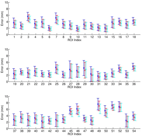
2.7 Errors of reconstructed deformation fields . . . 49

2.8 Errors of refined deformation fields . . . 51

2.9 Dice ratios of the P-R hierarchy on the NIREP dataset . . . 54

2.10 Dice ratios of the P-R hierarchy on the LONI dataset . . . 55

3.1 Comparison of pairwise and groupwise registration . . . 58

3.2 Subject images and the common space . . . 60

3.3 Atlas-based groupwise registration. . . 63

3.4 Conventional group-mean and sharp-mean . . . 66

3.5 MST and 18 elderly images . . . 74

(11)

3.7 Self-organized registration . . . 79

3.8 Image bundling and the hierarchical registration structure . . . 84

3.9 NIREP atlas . . . 87

3.10 Key points and importance sampling . . . 91

3.11 Local patterns of attributes . . . 92

3.12 Dice ratios of groupwise registration (I) . . . 97

3.13 Dice ratios of groupwise registration (II) . . . 98

3.14 Hierarchical groupwise registration . . . 100

3.15 Tissue atrophy detection . . . 102

4.1 Iterative multi-atlas labeling . . . 116

(12)

LIST OF ABBREVIATIONS

AD Alzheimer’s Disease

ADNI Alzheimers Disease Neuroimaging Initiative AP affinity propagation

CSF corticospinal fluid

GM grey matter

HAMMER hierarchical attribute matching mechanism for elastic registration ING iterative neighborhood graph

MDL minimum description length

MI mutual information

MR magnetic resonance

MRI magnetic resonance imaging MST minimum spanning tree NCC normalized cross correlation PDF probability density function PDFs probability density functions RBF radial basis function

RBFs radial basis functions ROI region of interest ROIs regions of interest

PCA principal component analysis PCG pre-central gyrus

SNR signal-to-noise ratio

(13)

TPS thin-plate splines

(14)

Chapter 1 Introduction

1.1 Significance of Image Registration

Without introducing hazardous ionizing radiation, magnetic resonance imaging (MRI) offers the capability to visualize internal structures of the human body in a non-invasive manner. The technique has thus been widely applied to numerous clinical and research works ever since it was invented decades ago. Brain magnetic resonance (MR) images, in particular, facilitate the diagnoses and the treatments for many neurological diseases thanks to the well rendered contrasts of brain tissues. Large-scale studies are enabled for investigating brain development (Caseyet al., 2000; Gieddet al., 1999; Lenroot and Giedd, 2006; Sowell et al., 1999b; Thompsonet al., 2000), maturation (Hollandet al., 1986; Sowell et al., 1999a; Paus et al., 1999, 2001), aging (Resnick et al., 2000; Raz et al., 2005), disease-induced anomalies (Frisoniet al., 2010; Laaksoet al., 2000; Polman

et al., 2011; Thompson et al., 1998), and for monitoring the effects of pharmacological

intervention over treatment time (Jack et al., 2004; Mulnard et al., 2000; Resnick and Maki, 2001).

(15)

spatiotempo-ral changes in brain tissue patterns that are difficult to identify visually. Meanwhile, technique advances help reduce the costs of MRI, thus large-scale populations of MR images are often employed in recent studies. To manually process and analyze large-scale populations of brain MR images, however, can be made difficult by (1) the rapidly increasing number of acquisitions; (2) the large size (or the dimensionality) of the im-age data; (3) the subtle changes of imim-age appearances; (4) the difficulty and the cost in recruiting human experts. As a result, many sophisticated computer-aided medical image analysis methods have been proposed in the literature, including image registra-tion (Glockeret al., 2011; Hajnal and Hill, 2010; Oliveira and Tavares, 2012; Rueckert and Schnabel, 2011), segmentation (Balafar et al., 2010; Heimann and Meinzer, 2009; Pham et al., 2000), disease-oriented classification (Aggarwal et al., 2012; Ecker et al., 2010; Kl¨oppel et al., 2008; Zhang et al., 2011), etc.

(16)

same template space, thus significantly reducing the costs in processing and analyzing large-scale image populations (Aljabaret al., 2009; Cuadra et al., 2004; Vemuri et al., 2003).

1.2 Brain MR Image Registration

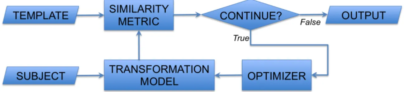
The registration of brain MR images has drawn abundant interest and also intensive investigations due to its importance in the area of medical image analysis. Most con-ventional methods regard the task of registration as a typical optimization problem, where a pair of moving subject and fixed template are often involved. The classical model of pairwise registration is illustrated by Figure 1.1, as the optimizer estimates the transformation, following which the subject is mapped to the space of the template in order to maximize the similarity between the two images. Typically, the solution to the transformation is attained in an iterative manner. In general, the optimization related to image registration tries to maximize the following objective function:

Objective(φ) = Similarity(T, S _◦φ) + Regularization(φ). (1.1)

(17)

the subject and the template are required to be mono-modal. Discussions of other images modalities and organs are outside the scope of this dissertation. • Similarity Metric. The similarity (or the distance) between the (transformed)

subject and the template can be computed in various ways, especially considering the fact that brain MR images are high-dimensional data. Though there are a huge number of voxels in each image and the anatomical variation of the images may be high, the similarity can be simply computed from the intensities of two images, i.e., as the inverse of the sum of squared differences (SSD) of intensities. More sophisticated measures and advanced features of image contexts can also contribute to the evaluation of the image similarity.

• Transformation Model. The transformation is a mapping between the image spaces of the subject and the template. The mapping of the rigid transformation, for example, allows rotation and translation of the subject. By incorporating scalings and shearings in addition, the model becomes the affine transformation. Non-rigid transformation affords unprecedented freedoms in deforming the sub-ject. This dissertation will focus on image registration that is related to non-rigid deformation. Further, the Lagrangian framework is adopted as the convention to denote the transformation in this dissertation. In particular, the transformation

φ(_·) is applied to register the moving subjectS with the fixed template T. Then,

φ(x) : ΩT →ΩS maps the template point x∈ΩT to the subject point φ(x)∈ΩS.

Similarly, the inverse transformation φ−1₍_y_{) : Ω}

S → ΩT maps the subject point

y_∈ΩS to the template point φ−1(y)∈ΩT.

(18)

the optimizer can also be perceived as a correspondence detector for the two images. The correspondence is defined as (1) two underlying points that are similar in appearances; (2) the two points that signify similar neuroanatomies. The optimizer estimates the transformation, following which individual points in the subject should be mapped to the coordinate locations of their correspondences in the template space. In this way, the optimizer is able to maximize the similarity between the transformed subject image and the template image.

• Multi-Resolution Hierarchy. Registration is regarded as an ill-posed opti-mization problem and suffers severely from the notorious curse of high dimen-sionality. Brain MR images are intrinsically high dimensional due to their large data size and the very abundant anatomical variations. The non-rigid transfor-mation, or defortransfor-mation, also requires a huge number of parameters for the sake of its representation. Therefore, to alleviate the aforementioned concerns, a multi-resolution strategy is often introduced by solving the registration problem hier-archically. For example, both the subject and the template can be down-sampled first, while a low-resolution transformation is computed. Then, the low-resolution transformation is up-sampled to be further optimized at the higher level, where high-resolution images should participate. The multi-resolution scheme allows more abundant image information (corresponding to varying resolutions) to be used by image registration, and results in a more robust estimation of the trans-formation.

1.2.1 Intensity-Based Methods

(19)

Figure 1.1: The classical model of pairwise image registration as a typical optimization problem.

similarity between the subject and the template can be calculated from image inten-sities directly. Though simple and straightforward, the inverse of the SSD of image intensities gives an effective image similarity measure in the Euclidean space. SSD adopts the assumption that noises in images are Gaussian distributed, and is success-fully applied in many state-of-the-art registration methods (Oliveira and Tavares, 2012). Several other intensity-based metrics are also available in the literature, including the statistical measure of normalized cross correlation (NCC) (Avants et al., 2008), the information-theory-based mutual information (MI) (Maes et al., 1997; Pluim et al., 2003; Viola and Wells III, 1997), minimum description length (MDL) (Davies et al., 2002), etc.

Diffeomorphic Demons (Vercauteren et al., 2009) is among one of the most popular intensity-based registration methods that are capable to handle brain MR images. The image similarity term in (1.1) is simply calculated as Similarity(T, S_◦φ) =_kT₋S_◦φ_k2

by Demons. After being combined with the regularization upon φ, the derivative ∂ _·

(20)

1.2.2 Feature-Based Methods

Correspondence detection, which is conveyed by image registration, can be challenged by high ambiguities in brain MR images if only intensity information is considered. Given two points that share the same intensity, it is risky to assert that they are corre-spondences to each other. In fact, though brain MR images offer good contrast between grey matter (GM) and whiter matter (WM), the intensities within a certain tissue can be very similar. To this end, it is often impossible to identify respective correspondences of neighboring points by using intensity information only. As an alternative, it is well known in computer vision research that correspondences can be better established by using sophisticated context features. The rule also applies in the case of brain MR image registration, to which correspondences between points (Maurer Jr et al., 1997), curves (Lyu et al., 2013), and surfaces (Jiang et al., 1992; Pelizzari et al., 1989) may contribute.

(21)

impor-tant locations are crucial for driving the correct alignment of corresponding anatomies of the two brains. For the sake of optimization, the selection of key points and the correspondence detection are further arranged into an iterative and multi-resolution scheme. With the progress of registration, more key points are devoted to the process as the correspondence detection becomes more accurate. The deformation field, which can be interpolated from the key points and their correspondences, thus approaches the desired solution gradually.

1.2.3 Deformation and Its Smoothness

The non-rigid transformation, or the deformation field, is usually expected to be phys-iologically meaningful and smooth in the registration of brain MR images. A simple criterion requires that the Jacobian determinant of the deformation field is positive everywhere. In this way, though the deformation allows free movement of individual points in the image space, it is guaranteed that no folding of brain tissues could possibly be introduced during the warping of the subject. Meanwhile, the smoothness of the deformation can be implemented in several different ways, e.g., via low-pass filtering of the deformation field.

(22)

of the deformation field.

• The deformation can also be parameterized as a collection of basis functions. B-Splines, for instance, are capable of representing the free-form deformation (Rueckert et al., 1999). In particular, for a certain control point in the image space, a B-Spline is attached to describe its contribution to the entire deforma-tion field. The set of control points should cover the whole brain volume, and often needs to be decided carefully. The deformation field, which is spanned across the entire image space, can be interpolated by integrating contributions from all control points. Other choices for the parametric modeling of the deformation field include but are not restricted to thin-plate splines (TPS) (Bookstein, 1989; Chui and Rangarajan, 2003), Fourier basis functions (Amitet al., 1991; Ashburner and Friston, 1999), and wavelets (Amit, 1994). Compared to non-parametric mod-eling, parametric modeling is able to reduce the number of parameters that are needed for the representation of the deformation field. Thus, the optimization of the registration usually becomes less challenging. Also, most parametric model-ing provides subtle controls upon the smoothness when the deformation field is interpolated.

(23)

and the fluid styles are different, they can sometimes be combined and utilized as a hybrid. In particular, the incremental of the deformation estimated in every iteration complies with the smoothness constraint in the fluid style, while the it-eratively integrated overall deformation can be regulated by the elastic constraint as well.

1.2.4 Performance Evaluation

It is necessary to evaluate the performances of brain MR image registration, before the registration outputs can be potentially used by the following clinical applications and research studies. The lack of prior knowledge or the ground truth, however, leads to the dilemma that the performance evaluation could be non-trivial. The evaluation often starts from the assessment of the robustness of the registration results. Experts with minimal training can easily conclude whether a registration is satisfactory by visually inspecting the similarity between the deformed subject and the template images. The robustness of image registration is important in that the registration method is expected to handle a large-scale population of images automatically. Manual inspection obviously interrupts the pipeline in processing images and requires additional cost.

(24)

of the Alzheimer’s Disease (AD) (Camara et al., 2008).

The annotations of anatomical structures provide a convenient way to evaluate registration accuracy. Note that the purpose of image registration is to correctly align corresponding anatomies. Thus, the consistency or overlapping of identical anatomical structures after registering the subject to the template space is a natural indicator of the registration quality. For instance, by (manually) labeling regions of the same anatomical role but from the deformed subject and the template, respectively, the overlap of the two regions can be captured by the Dice ratio

RD(Region1,Region2) =

2_×Vol(Region₁_∩Region₂)

Vol(Region₁) + Vol(Region₂). (1.2)

Here, the operator Vol(_·) computes the volume of the underlying anatomical region. Be-sides the Dice ratio, other measures (e.g., the Jaccard ratio) may be applicable as well. The registration accuracy metric can also extend to incorporate more corresponding anatomical structures, including landmarks, curves, surfaces, etc.

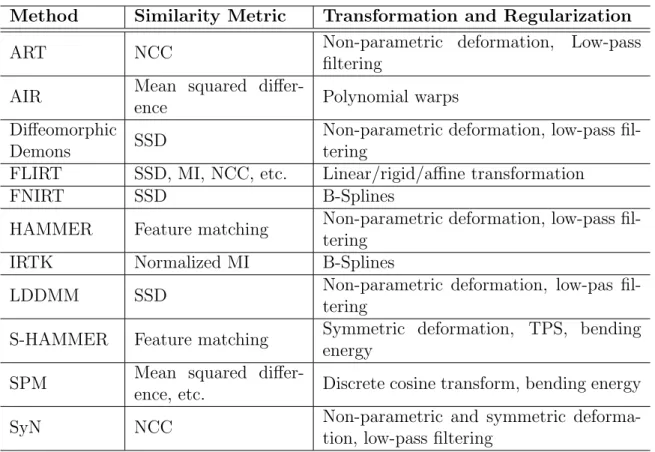
To end the retrospect of the literature, a list of typical registration methods for brain MR images is provided in Table 1.1. Also, it is worth noting that a comprehensive investigation of performances of individual registration methods is reported in Klein et al. (2009). Systematic understanding and surveys of the current status of medical image registration are also available in the literature (Hajnal and Hill, 2010; Oliveira and Tavares, 2012; Rueckert and Schnabel, 2011).

1.3 Limitations of Conventional Methods

(25)

Method Similarity Metric Transformation and Regularization

ART NCC Non-parametric deformation, Low-pass

filtering

AIR Mean squared

differ-ence Polynomial warps

Diffeomorphic

Demons SSD

Non-parametric deformation, low-pass fil-tering

FLIRT SSD, MI, NCC, etc. Linear/rigid/affine transformation

FNIRT SSD B-Splines

HAMMER Feature matching Non-parametric deformation, low-pass fil-tering

IRTK Normalized MI B-Splines

LDDMM SSD Non-parametric deformation, low-pas

fil-tering

S-HAMMER Feature matching Symmetric deformation, TPS, bending energy

SPM Mean squared

differ-ence, etc. Discrete cosine transform, bending energy

SyN NCC Non-parametric and symmetric

deforma-tion, low-pass filtering

Table 1.1: Summary of state-of-the-art pairwise registration methods for brain MR images. Only exemplar methods are reported in this table, including: ART (Ardekani and Bachman, 2009), AIR (Woodset al., 1998b,a), Diffeomorphic Demons (Vercauteren et al., 2009), FLIRT (Jenkinson and Smith, 2001; Jenkinson et al., 2002), FNIRT (Andersson et al., 2008), HAMMER (Shen and Davatzikos, 2002), IRTK (Schnabel et al., 2001), LDDMM (Beget al., 2005), S-HAMMER (Wuet al., 2012d), SPM (Friston et al., 2011), and SyN (Avantset al., 2008).

(26)

spaces, which are not necessarily related to the image population under consideration, may also provide convenient alternatives.

Images in the population can be regarded as individual subjects and handled by pairwise registration in either the round-robin or parallelized manner. The registration tasks of individual subject images are essentially independent of each other. However, it is known that two similar subject images (i.e., denoted by S1 and S2), when

regis-tered with the same template, should have similar deformation fields. This property is unfortunately ignored when applying pairwise registration to a large-scale population of images. Even though S1 and S2 are very similar in appearances and deformations,

their registration with the template is independently considered. However, it would be desirable for the two subject images to share certain information during the registration process. For example, the registration of S1 (or S2) might be a good approximation

of the registration of S2 (or S1). In other words, to register one of them could well

initialize the registration of the other.

(27)

1.4 Thesis

Thesis: Registration of brain MR images in large-scale populations benefits from

utiliz-ing information from the entire population, instead of from the subject and the template

only.

This dissertation investigates ways of incorporating information contributed by the entire image population into solving the registration problem. In particular, two specific aims are proposed to improve brain MR image registration.

• Specific Aim 1: Pairwise registration can be improved by utilizing the guidance from other images in the population. Instead of registering the subject with the template directly in the conventional style of pairwise registration, the subject can initiate its registration by using guidance provided by other images (namely the intermediate images) in the population. The guidance of the intermediate images

helps the subject to identify its deformation towards the template more easily. Thus the registration of the subject with the template becomes more robust and accurate in the end, compared to direct registration of the two images.

• Specific Aim 2: The large-scale population of brain MR images can be registered towards their common space in a groupwise manner. Groupwise registration sig-nificantly differs from the traditional pairwise registration, in that the designation of the template, as well as its bias, is completely avoided. However, by iteratively optimizing the coherence of the population, groupwise registration is capable of deforming all images to the common space of the population. Meanwhile, the similarity between each pair of warped subjects is maximized, as all images are registered with each other with respect to the common space.

(28)

• Two types of guidance from the intermediate images, namely the image-scale guidance and the patch-scale guidance, are investigated for guiding the pairwise registration of a certain subject with the template and improving registration performance;

• The image-scale guidance allows the subject to seek help from the intermediate image in estimating its own deformation towards the template, in that the in-termediate image is required to be similar to the subject and thus shares similar deformations with respect to the template;

• In the setting of patch-scale guidance, individual patches in the subject flexibly predict their associated deformations with respect to the template, in accordance with the guidance provided by different intermediate images and their correspond-ing patches;

• The importance and advantages of groupwise registration are addressed, as in groupwise registration all subject images in the large-scale population are warped to an unknown common space where the atlas of the population can be con-structed;

• With a mean image to represent the common space, groupwise registration is feasibly implemented by a set of pairwise registrations of individual subjects and the mean, while the sharpness of the group-mean is proven to be significantly important in terms of the quality of groupwise registration;

(29)

• With an objective function to capture the variation of all images with respect to the unknown common space, groupwise registration is able to directly optimize the objective function by simultaneously estimating the deformation fields for all subjects; meanwhile, correspondences of points from individual subjects are established via the implicit common space;

• By incorporating information of the entire population, overall registration quality is improved, thus benefiting other related applications, e.g., to propagate anatom-ical labeling from the known images to the unknown images more precisely after all images are registered.

1.5 Overview of Chapters

The remaining chapters of this dissertation are organized as follows.

• Chapter 2 investigates the utilization of the guidance, provided by the intermedi-ate images, in pairwise registration of the subject with the templintermedi-ate. The scales of the guidance, i.e., at the image or the patch scale, are further addressed and compared. The guidance from the intermediate images provides good initial-ization for the subject to estimate its deformation towards the template. The initialized deformation can be refined efficiently and effectively, and thus enhance the accuracy of pairwise registration significantly.

(30)

be aligned with each other more accurately in the common space compared to pairwise registration, though the problem of groupwise registration is much more complicated due to the population size.

• Chapter 4 demonstrates that improved registration, i.e., by incorporating infor-mation from the entire population, can benefit the multi-atlas labeling technique to generate more reliable segmentation outcomes. Multi-atlas labeling, a state-of-the-art method, is capable of propagating anatomical labels from the known atlas to other unknown images for the sake of automatic segmentation. In that the at-lases and the to-be-segmented images are registered more precisely, the resulting segmentation provided by multi-atlas labeling is also improved in the context of brain MR images.

• Chapter 5 concludes the entire dissertation. In general, this dissertation inves-tigates the contributions of large-scale populations towards image registration. The entire population benefits the conventional pairwise registration between two images, due to the guidance from other intermediate images in the popula-tion. Moreover, from the perspective of groupwise registration, all images in the population can be registered simultaneously and accurately.

1.6 Summary

(31)

(32)

Chapter 2 Population Guidance in Pairwise

Registration

2.1 Overview

When applying the conventional pairwise registration methods to a large-scale popula-tion of brain MR images, the typical scenario requires researchers to specify a certain template first and then register all images with the template. Regardless of the order in handling subject images, the registration of each individual subject is generally in-dependent of the others, as only a specific subject and the template are involved in any particular pairwise registration task. The performance of this straightforward scheme, namely thedirect registration of the subject, could be undermined by the complexities in (1) evaluating the similarity of high-dimensional image data and (2) optimizing a huge number of parameters to represent the deformation field. The direct registration could even fail if the subject and the template differ significantly in appearances. To this end, the desire for high-performance registration has inspired enormous efforts for the improvement of existing registration methods.

(33)

is utilized by a family of methods to initiate optimization and produce better registra-tion outputs in the end. Specifically, both the template and the to-be-registered subject are incorporated by a population; other images in the population are termed as the in-termediate images, whose registration with the template are presumed to be known already. Then, for the subject image under consideration, the guidance towards its registration with the template originates from the intermediate images in the popu-lation. In particular, two images that are similar in appearances should have similar deformations when registered with the same template. Thus, after identifying a certain intermediate image from the population that is similar with the subject in appearances, the subject initiates its own registration with the template immediately, by using the deformation field that has been pre-estimated for that specific intermediate image.

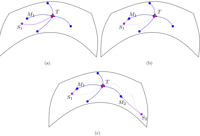
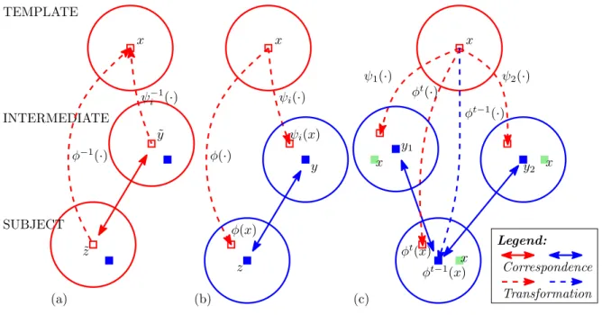
The contribution from the intermediate image, which is categorized as the image-scale guidance here, is illustrated by Figure 2.1. Given a large-scale population of brain MR images, a high-dimensional manifold is often instantiated to characterize the distri-bution of the entire population (Aljabaret al., 2012). Images that are similar in appear-ances are spatially close to each other within the manifold. Meanwhile, the geodesic along the manifold connects a certain pair of images, and represents the deformation pathway for the registration between them. Figure 2.1(a) illustrates an image manifold and enumerates several exemplar images that are annotated by individual nodes (i.e., red for the template, purple for the subject, blue for the intermediate images). The geodesic arrow denotes the deformation pathway, following which a non-template image is registered with the template. The intermediate images are pre-registered with the template, thus the deformation pathways in blue are known already.

The direct estimation of the deformation in purple that registers the subject S1

(34)

image M1 to initialize its own registration. That is, S1 first registers with the

inter-mediate image M1, and then follows the existing pathway from M1 to T to complete

its registration with the template. The overall deformation of S1 is thus derived from

the integration of two deformation segments that correspond to the two registration sub-tasks. It is worth noting that the intermediate image M1 is required to be similar

to S1 in this case. Thus the deformation segment from S1 to M1 is relatively short,

while the segment fromM1 toT contributes to the majority of the overall deformation

forS1. In other words, the deformation that registers M1 with T can be regarded as a

well-functioning approximation (as well as initialization) to registering S1 with T.

The image-scale guidance contributed by the intermediate image M1 is able to

al-leviate difficulties in registering the subjectS1 with the template T directly. Given an

existing deformation that registers M1 to T reliably, the remaining task for S1 is to

find the deformation segment from S1 toM1 only. The length of the to-be-determined

segment of the entire deformation pathway is shortened significantly. A short pathway usually implies that the registration could be handled more easily, complying with the observation that the registration between similar images faces many fewer challenges in optimizing the deformation field. After integrating two segments into a single defor-mation, the subject is able to further refine the defordefor-mation, i.e., via state-of-the-art registration methods, in effective and efficient manners.

The guidance from the intermediate images also allows registration to assess diffi-culties of individual tasks and then assign priorities to register images in the population adaptively. In the case illustrated by Figure 2.1(c) for example, the direct registration of the subjectS2 with the template T could be challenging due to the high anatomical

variation and the lengthy deformation pathway between them. However, with the in-troduction of the intermediate imageM2, the registration ofS2 is decomposed into two

(35)

T

S1

M1

(a)

S1

M1 T

(b)

S1

M1 T

M2

S2

(c)

Figure 2.1: The manifold of the image population and the image-scale guidance in pairwise registration: (a) The subject S1 is registered with the template T directly

regardless of other intermediate images (includingM1) in the population; (b)

Alterna-tively S1 utilizes the guidance provided by M1 to initiate its registration with T; (c)

The registration of S2 with T is decomposed into two relatively easy-to-solve problems

with the introduction ofM2, i.e., from S2 toM2 and from M2 toT, respectively. Red

nodes correspond to the templates, blue for the intermediate images, and purple for the subjects. Curved arrows correspond to the deformation pathways that register the linked pairs of images.

sub-tasks are obviously less difficult than the direct registration of S2 with T. To this

end, the optimal strategy in handling S2 is to defer its registration until the guidance

associated withM2 has become available. Therefore, from the perspective of the entire

population, images that are more similar to the template (e.g., M2) should be

regis-tered at higher priorities than other images that are less similar to the template (e.g.,

S2). In this way, those images registered at earlier stages might be recursively utilized,

(36)

overall registration performance evaluated upon the entire image population can thus be improved.

Granularity of Guidance. Though above discussions are focused onimage-scale guidance, the intermediate images are capable of contributing towards the registration of the subject image in the patch-scale manner. The two types of guidance differ significantly in terms of their granularities. For example, once the subject has identified the intermediate image (similar in appearances), the image-scale guidance is provided by the intermediate image within the entire image space. The rationale is that similar images (in appearances) should have similar deformation fields when registered with the same template. On the other hand, the patch-scale guidance relies on the fact that the deformations of two patches from the subject and the intermediate image are highly correlated, if the appearances of the two patches are similar (Wanget al., 2013b). Therefore, for individual patches of the subject, their correspondences may come from patches belonging to different intermediate images. By reducing the granularity of the guidance from image to patch, the patch-scale guidance allows the subject to utilize all intermediate images in the population for predicting its own registration more flexibly.

(37)

effec-tive refinement, the final deformation is able to register the subject with the template more accurately, compared to the traditional direct registration scheme.

The rest of this chapter is organized as follows. In Section 2.2, more details related to image-scale guidance are provided. Then, patch-scale guidance is proposed and elaborated in Section 2.3. A brief summary is available in Section 2.4 to conclude this chapter.

2.2 Image-Scale Guidance

Incorporating the intermediate images in the population alleviates many of the chal-lenges encountered by the direct registration of the subject with the template. A critical problem to be resolved here is the identification of the source of the guidance, or the optimal intermediate image for a certain subject. In particular, two criteria need to be satisfied to qualify the intermediate image, which are that it (1) should be similar to the subject in appearances and (2) is registered with the template already. The image-scale guidance is often utilized in two directions (Jia et al., 2012b), i.e., (1) selecting the intermediate image from the population to best approximate the subject, and (2) generating the subject-specific intermediate image via simulation.

2.2.1 Intermediate Image: Selection

The optimal intermediate image can be cherry-picked from the image population (Dalal et al., 2010; Hamm et al., 2010; Jia et al., 2011b; Munsell et al., 2012; Wolz et al.,

(38)

the literature, simple metrics (e.g., SSD and MI) are often adopted to capture image similarity. More sophisticated measures associate the similarity with the deformation field between images (Beget al., 2005; Joshiet al., 2004). The manifold of images is then approximated by graph-based structures, where nodes correspond to individual images and edges reflect similarities between images. Different from the full connection of all pairs of images, the graph-based structure only allows similar images to be connected and thus registered directly. The deformation pathway between images that are not directly linked is estimated by concatenating all edges of the shortest path between the two images in the graph-based structure. Thus, for a to-be-registered subject, its deformation is predictable given its path towards the template in the graph-based structure. In other words, the intermediate images, which correspond to nodes along the path from the subject to the template, provide guidance to register the subject under consideration.

(39)

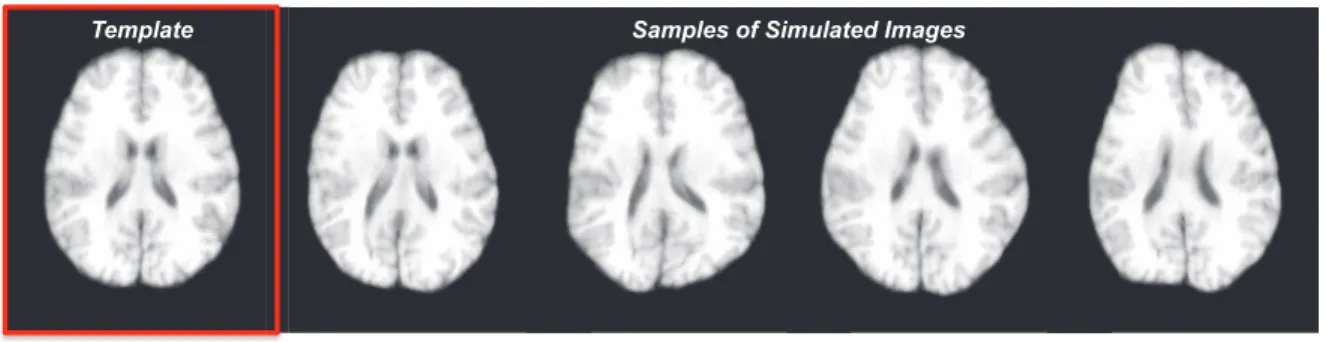
With SSD to describe the distance between each pair of images, a minimum spanning tree (MST) is instantiated in Figure 2.2(a) to model the distribution of the entire population. The root of the tree serves as the template, to which all other simulated images need to be registered. The distribution in the tree can be verified via principal component analysis (PCA). In Figure 2.2(b), all images in the population are projected on a 2D plane, which is spanned by the first two principal components identified in PCA. The root and the three branches, which lead to the structure of the tree, are clearly observable in the PCA output.

(40)

(a)

(b)

(41)

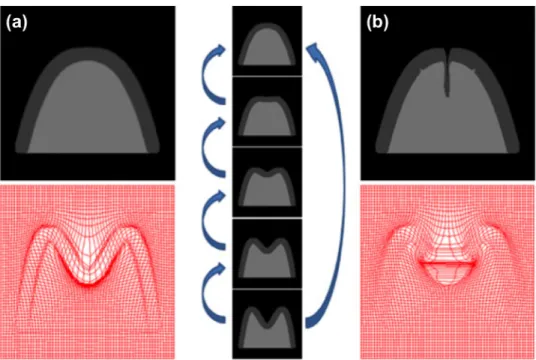
Figure 2.3: The direct registration of the subject leads to a failure in (b), while the subject essentially locates the correct deformation pathway with the guidance from the intermediate images in (b).

2.2.2 Intermediate Image: Generation

(42)

image. Moreover, the intermediate image is highly similar to the subject in appearance, in that the deformation field for its generation encodes the appearance of the subject already. As a result, the registration of the subject to the intermediate image is easy to solve, while the entire deformation pathway from the subject to the template can be integrated and refined afterwards.

2.3 Patch-Scale Guidance

2.3.1 Motivation

It is effective to improve the performances (i.e., robustness and accuracy) in registering the subject with the template by introducing additional intermediate images in the population. The utilization of the image-scale guidance, as in Section 2.2, considers the entire image as a whole. A fundamental assumption for the image-scale guidance is that images with similar appearances should have similar deformations when registered with the same template. The assumption is closely related to the manifold instantiated for describing the large-scale population of images (e.g., Figure 2.1). Though geodesics upon the manifold are perceived to represent deformation pathways between neigh-boring images, the theory is challenged especially by the high-dimensional images and deformations. In fact, it is known that a tiny perturbation in the appearance of the images (and thus their mapped locations on the manifold) may possibly result in a very different deformation for registration (Modersitzki, 2004).

(43)

similarity. The subject might share common anatomical structures with the interme-diate image in certain gyri or sulci, where the guidance from the intermeinterme-diate image is trustworthy; at the same time, they may also differ significantly in other areas where the guidance could even be harmful. A simple illustration is provided in Figure 2.4, where a new subject is simulated (and highlighted by the blue rectangle) in addition to the dataset in Section 2.2.1 and Figure 2.2. The new subject differs significantly in appearance from any other image in the population, implying that the intermediate image can hardly be acquired for providing guidance at the scale of the entire image.

(44)

different intermediate images for individual points in the image space.

Although it is hard to utilize image-scale guidance for the specific new subject in Figure 2.4, patch-scale guidance helps its registration with the template due to the high flexibility in accessing the intermediate images. In particular, due to a certain point on the left half of the new subject, its correspondence can be easily identified from the intermediate image at the end of Branch I, e.g., by comparing appearances within the two respective patches circled in green (c.f. Figure 2.4(a)). The deformation associated with the subject point under consideration is then predictable, in that the subject point shares a common correspondence in the template space with the identified point in the intermediate image. Meanwhile, for the point in the right half of the subject image (e.g., encircled by the yellow patch), its correspondence in the template, as well as the associated deformation, is also revealed with respect to the guidance from another intermediate image (i.e., at the end of Branch III). Note that the patch-based correspondence detection is conducted within the neighborhood of each point-of-interest, since only local correspondence is meaningful in non-rigid brain MR image registration.

2.3.2 The Prediction-Reconstruction Protocol

To effectively utilize the patch-scale guidance from the collection of the intermedi-ate images and apply it towards brain MR image registration, a novel prediction-reconstruction strategy, namely the P-R protocol, is proposed in Wang et al. (2013b). The P-R protocol consists of two coupled steps:

1 Predict the deformations associated with a subset of key points, which are scat-tered in the image space to cover the entire brain volume;

(45)

(a)

(b)

(46)

deformations to register the subject image with the template.

In the prediction step, it is critical to establish point-to-point correspondences be-tween the subject and the template, by utilizing the highly reliable correspondences identified between the subject and the intermediate images. To this end, the patch-based sparsity learning technique, which is widely applied in computer vision (Wright et al., 2010), is applied here. For a specific subject point, it aims to estimate the linear

and sparse representation of its surrounding patch given all possible candidate patches from the intermediate images. The optimal linear representation determined by the sparsity learning locates a sparse set of intermediate patches, the appearances of which are highly similar to the subject patch under consideration. Therefore, all center points of the intermediate patches qualified by the sparsity learning can be regarded as the cor-respondence candidates of the subject point, and then help identify the corcor-respondence of the subject point in the template image. The subject-template point correspondence predicts the (local) deformation, following which the specific subject point is expected to deform.

(47)

the reconstructed deformation field complies with the smoothness constraint, in order to suppress unrealistic warping (i.e., folding) of brain tissues.

2.3.3 Prediction of Correspondences

It is critically important to predict the correspondence, as well as the associated de-formation, of each key point in the image space. For convenience, mathematical nota-tions with respect to the P-R protocol are introduced first. In particular, the subject

S needs to be registered with the fixed template image T following the deformation

φ(_·) : ΩT → ΩS, while the point x ∈ ΩT in the template space locates its

corre-spondence at φ(x) _∈ ΩS in the subject image space. Conversely, φ−1(·) is capable

of deforming the template towards the subject image space. To help estimate φ(_·), the patch-scale guidance is contributed by the collection of the intermediate images {Mi|i = 0,· · · , m}. Given each Mi, the deformation ψi(·) that registers it with the

template is already known. That is, ψi(x) ∈ ΩMi indicates the correspondence of the

template point x _∈ ΩT. Note that the template T is also referred as M0, as ψ0(·) is

simply an identity transform that registers the template to itself. For easy reference, a list of important variables here is summarized in Table 2.1. Moreover, since only the prediction of the non-rigid deformation is investigated here, all images are necessarily pre-processed, including being aligned to a common space by affine registration (i.e., FLIRT (Jenkinson and Smith, 2001; Jenkinsonet al., 2002)).

The deformation is predictable in that point-to-point correspondences can be iden-tified from similar patch-scale appearances between images. Figure 2.5 helps illustrate the rationale of the patch-scale guidance. In Fig. 2.5(a) particularly, three individual patches (in the top-bottom order) from the template T, a certain intermediate image

(48)

Variable Note

T Template image

S Subject image

Mi The i-th intermediate image (i is the index)

ΩT,ΩS,ΩMi Individual image spaces

x Template point

y,y˜ Points in the intermediate images

z,z˜ Points in the subject image

t Resolution

φ(_·) Transformation field to register _S with _T

ψi(·) Transformation field to register Mi with T

~

φ, ~ψ_i Signature vectors of φt(x) andψ_i(x)

~

u, ui Confidence of ψi(x) in prediction

~

ξ, ~θij Signatures of patches at φt−1(x) andyij

~

v, vij Confidence of yij in prediction

rc Maximal radius allowed in correspondence detection

~

w, wij,W Confidences of combined predictions

k(_·),K RBF kernel function and kernel matrix

σ, c Control the size of the support of k(_·)

~

γx,Γ RBF kernel coefficients

Φ Predicted transformations

Table 2.1: Summary of important variables with respect to the Prediction-Reconstruction protocol.

losing generality, x and ˜y are defined to be correspondences to each other such that ˜

y=ψi(x) or x=ψi−1(˜y). Immediately this leads to

Proposition 1 If y˜_∈ΩMi and z˜∈S are correspondences to each other, then

φ−1(˜z) = ψ_i−1(˜y). (2.1)

Proof 1 Given the facts that (1) y˜and z˜are correspondences to each other, (2) xand ˜

z are correspondences to each other, the correspondence relationship could be established

(49)

consideration share similar appearances in their surrounding patches. Therefore, the

proposition is derived following (1) x=ψ_i−1(˜y) and (2) x=φ−1(˜z) accordingly.

The proposition above allows the prediction ofφ−1₍_·_{) from the inverse of the}

collec-tion _{ψi(·)}. The model is further improved to predict φ(·) directly fromψi(·), instead

of its inverse. As in Figure 2.5(b), there is

Proposition 2 If (1) y_∈ΩMi and z ∈S are correspondences to each other AND (2)

y is spatially close to ψi(x), then

φ(x)₋z =_∇φ(x) (_∇ψi(x))

−1

(ψi(x)−y), (2.2)

where _∇ indicates the Jacobian operator.

Proof 2 As y is spatially close to ψi(x), it is natural to assume that y = ψi(x+δx)

where δx is a infinitesimal perturbation of x. Moreover, it is implied by ψi(·) that the

point (x+δx) locates its correspondence as y. Thus the points (x+δx) and z are also correspondences to each other, via the bridge of y_∈ΩMi:

y = ψ_i(x+δx) = ψ_i(x) +_∇ψ_i(x)δx+_O(δxTδx), (2.3)

z = φ(x+δx) = φ(x) +_∇φ(x)δx+_O(δxTδx). (2.4)

After subtracting the two equations and eliminating the perturbation variableδx, it leads

to the conclusion

(_∇ψi(x))−1(y−ψi(x)) = (∇φ(x))−1(z−φ(x)), (2.5)

(50)

x x

˜ y

˜ z

φ−1₍_·₎

TEMPLATE

SUBJECT INTERMEDIATE

z

ψi(x)

φ(x)

(a) (b)

Correspondence

Transformation Legend: y

ψ−_i1(·) ψi(·)

φ(·)

x

φt₍_·₎

φt−1₍_·₎

ψ1(·) ψ2(·)

φt−1₍_x₎

φt₍_x₎

(c) y1 y2 x x x

Figure 2.5: Illustration of the predictability of the deformation: (a) The correspon-dence between the template point x and the subject point ˜z is established as both points identify ˜y as their correspondence in the intermediate image; (b) The subject deformationφ(x) is predictable from the intermediate deformationψi(x), ify andz are

correspondences to each other; (c) Multiple correspondence candidates of y might be detected, thus resulting in multiple predictions upon the subject deformation φ(x).

The rule in Proposition 2 allows the prediction of φ(x) from the intermediate col-lection _{ψi(x)} of the intermediate images. All variables (i.e., i, y, x, and z in (2.2))

need to be handled carefully for brain MR image registration. In particular, a set of key points is selected from the template image space, with more details regarding the selection of key points provided in Section 2.3.5. Each key point is then fed as an instance of the variablexto (2.2). Furthermore,z is related to the tentative estimation of φ(x); thus (2.2) is converted to the incremental optimization style as

φt(x) :=φt−1(x) +_∇φt−1(x) (_∇ψi(x))−1(ψi(x)−y). (2.6)

Here, t records the timing in optimizing φ(_·). The term _∇φt−1₍_x_{) is used to}

(51)

∇φt−1(x) mildly. The variables i(as well asψi(x)) and ywill be determined later, such

thaty_∈ΩMi is the correspondence to the previously estimated φt−1(x)∈ΩS given the

patch-scale appearances of the two center points.

Given the key point x, several intermediate images with their individual contribu-tions asψi(x) might be available. Moreover, multiple instances of y can potentially be

identified as correspondences toφt−1(x) as well. Though the number of correspondences can be arbitrarily reduced to 1 for each instance ofx, allowing multiple correspondences can greatly improve the robustness and the accuracy for correspondence detection (Chui and Rangarajan, 2003). To this end, the sparsity learning technique (Wright et al., 2010) is applied for the determination of i and y, respectively. In general, the sparsity learning technique allows multiple, yet only a limited number of, instances ofψ_i(x) and

y to contribute to the prediction in (2.6). Meanwhile, varying confidences are attained for the instances of ψi(x) and y that are active in the prediction. The product of the

confidences ofψi(x) andy is further regarded to measure the reliability of the resulted

predictions. All key points and their multiple predicted deformations, along with the varying confidences, are passed to the reconstruction of the dense deformation field in Section 2.3.4.

Determination of i and ψi(x)

The correspondence betweenφt−1(x) and yimplies that the locations of the two points should be close to each other, especially in brain MR images after affine registration. Therefore,ψi(x) better predicts φt(x) if the two deformations are more similar. In Fig.

2.5(c), for example, the pointφt−1(x) is assumed to identify its correspondencey1 from

M1 and another correspondence y2 from M2. However, the challenges in determining

y1 and y2 are different concerning ψ1(x) and ψ2(x). As ψ2(x) is closer to φt(x) than

(52)

thus should be conducted in a much larger area in that_ky1−φt−1(x)k>ky2−φt−1(x)k.

In this case, ψ2(x) is obviously a better selection for the sake of predicting φ(x).

In order to determine aψi(x) that is similar toφt(x) and compute the accompanying

confidence, the sparse representation of φt(x) over the dictionary spanned by ψi(x) is

investigated. Assuming that φt(x) and ψi(x) are signified by the vectors ~φ and ψ~i,

respectively, the sparsity learning aims to solve

~

u= arg min

~

u k

~

φ₋Ψ~u_k2+α_k~u_k1,

s.t. Ψ= [ψ~1,· · ·, ~ψi,· · · , ~ψM],

~

u= [u1,· · · , ui,· · · , uM]T,

u_i _≥0,_∀i.

(2.7)

Here,~uindicates the vector of the coefficients for the linear representation ofφ~given the dictionary Ψ, which consists of potential contributions from all intermediate images. The l1 constraint k~uk1, weighted by the non-negative scalar α, favors a sparse subset

of column items from Ψ to represent φ~. The coefficient ui, yielded by the sparsity

learning, also acts as a similarity indicator between ~φ and ψ~i (Wright et al., 2010).

To attribute signatures to both φt(x) and ψi(x), the corresponding deformations

are vectorized into φ~ and ψ~i, respectively. On the other hand, φ~ cannot be acquired

directly, in thatφt(x) is still pending for estimation. As an alternative, the signature φ~

is generated from φt−1(x), based on the assumption of mild changing between φt−1(x) and φt(x). In general, via the optimization in (2.7), several intermediate images are identified (or activated), with their contributions _{ψi(x)} and the non-negative

coeffi-cients_{ui}, for the sake of the prediction of φt(x). The term ui is further regarded as

(53)

Determination of y

Candidates of y can be identified via the correspondence detection, centered at the location ofφt−1₍_x_{), within each active intermediate image after the determination of}_i_.

For convenience, all possible candidates ofyare annotated by_{yij}, asyij indicates the

j-th candidate from the i-th intermediate image. The candidate collection _{yij} often

consists of each grid point yij ∈ ΩMi if kφt−1(x)−yijk ≤ rc and rc is the maximally

allowed radius for correspondence detection. The signatures of the pointsφt−1₍_x_{) and}

yij are defined as ξ~and ~θij, respectively, as the similarity between the two points can

thus be acquired by comparing their signature vectors. In particular, the same sparsity learning technique is used for the purpose

~v = arg min

~v k

~

ξ₋Θ~v_k2+β_k~v_k1,

s.t. Θ= [_{· · ·} , ~θ1j,· · ·, ~θij,· · · , ~θM j,· · ·],

~v = [_{· · ·} , v1j,· · · , vij,· · · , vM j,· · ·]T,

vij ≥0,∀i, j.

(2.8)

In (2.8), the matrix Θ indicates the dictionary of contributions from the candidate collection_{yij}, the vector~v records the coefficients for the linear sparse representation

of ~ξ given Θ, and the non-negative scalar β controls the sparsity of~v. The vectorized patch is defined as the signature (i.e., ~θij) for the center point (i.e., yij). Then, vij

captures the similarity between the two patches centered at φt−1₍_x_{) and} _y

ij. Higher

vij obviously implies that the correspondence between φt−1(x) and yij is more reliable

given their individual patch-scale appearances. As the result, vij is regarded as the

confidence for predictingφt(x) from yij.

(54)

consistency in correspondence detection is enforced via the l2,1-norm constraint (Liu

et al., 2009). In particular, the optimization problem in (2.8) is modified as

V= arg min

V k

Ξ₋ΘV_k2+β_kV_k2,1,

s.t. Ξ= [_{· · ·} , ~ξx+∆,· · ·],k∆k ≤,

Θ= [_{· · ·} , ~θ1j,· · · , ~θij,· · · , ~θM j,· · ·],

V= [_{· · ·} , ~vx+∆,· · ·],k∆k ≤,

vx+∆,ij ≥0,∀∆,∀i,∀j.

(2.9)

(2.9) aims to detect correspondence candidates for the centering point x, as ∆ in the subscript is associated with the point (x+ ∆) that is neighboring x. Similarly, ξ~x+∆

represents the signature vector for (x+ ∆). The matrix Ξ captures signatures for all points that are located within the radius of to the point x, while their representation coefficients onΘ are stored in individual columns of the matrix V. Identical to (2.8), the coefficient vector for (x+ ∆), namely vx+∆,ij is encouraged to be sparse.

Mean-while, neighboring points are inclined to share similar coefficients, as their patch-scale appearances could not change drastically. Therefore, besides the l1 constraint, the l2,1

constraint to the matrix V (Liu et al., 2009) is enforced. That is, each column of V satisfies the sparsity requirement, while the sparsity patterns of individual columns are expected to be highly similar. Finally, the column for ∆ = 0 in V tells all possible correspondence candidates of the pointφt−1(x).

Any arbitrary combination ofψi(x) andyij yields an attempt in predictingφt(x). In

particular, the confidencewij is defined for the attempt as the product of the confidences

of ψi(x) andyij, orwij =uivij. The sparsity enforced in selecting ψi(x) andyij results

(55)

way, the method can (1) avoid local minima if only acquiring a single but incorrect prediction for the key point, and (2) suppress a majority of predictions of low reliability. The confidence of each key point is further normalized by wij ←wij/Pwij, to impose

the same priors on all key points.

The order of determining i first and then y provides good scalability in handling a large-scale population of (intermediate) images. Specifically, the determination of

i can be much more efficient than y, in that the column size of the dictionary Ψ is identical with the number of intermediate images, or _O(m). Meanwhile, multiple correspondences may exist in even a single intermediate image. The dictionary Θ has to enumerate all possible instances ofy, and thus increases the column size to_O(r3

cm),

as r_c represents the radius in searching for correspondences. By determining i first, the number of activated intermediate images, only from which the contributions to the determination of y should be counted, is well controlled. Thus, the complexity in determining y is well scaled regardless of the size of the collection of the intermediate images, as most intermediate images aredeactivated already in the determination ofy.

2.3.4 Reconstruction of Deformation Field

The dense deformation field is reconstructed to fit the multiple predictions of all key points. To this end, the radial basis function (RBF) provides a feasible means for the representation of the deformation field. Suppose that the RBF kernel function is k(_·) and ~γ_x is the radial basis function (RBF) coefficient vector for the key point x, the dense field associated with the arbitrary location x0 _∈Ω_T is then computed by

φ(x0) =X

x

k(_kx0₋x_k)~γx. (2.10)

(56)

-th row and -then-th column is calculated by feeding the Euclidean distance between the

m-th and then-th key points to the kernel functionk(_·). If only a single prediction was ever attempted for each key point, the residuals for the dense field to fit the predicted deformations of all key points could then be easily computed in the matrix form as kΦ₋KΓ_k2. Here, the predicted deformation (in the transposed row vector form) of them-th key point is recorded in them-th row ofΦand its transposed RBF coefficient vector in them-th row ofΓ.

In order to accommodate multiple predictions of each key point, the expanded matrix Φ and the confidence matrix W are introduced for fitting. All predictions, as well as the confidences, are enumerated in Φ and W. Supposing that the p-th row of Φrecords a certain prediction for the m-th key point weighted with the confidencew_ij, the entry ofWat the junction of thep-th row, and the m-th column is set tow_ij while all other entries in the p-th row are zero. The overall residuals in fitting predictions, weighted by varying confidences, then become_kΦ₋WKΓ_k2_.

Smoothness regularization is critically important to the reconstruction of the dense field, in order to suppress any unrealistic warping that might be applied to brain tissues (Rueckert and Schnabel, 2011). To this end, the kernel functionk(_·) is usually designed in the style of low-pass filters (Myronenko and Song, 2010). Further, if K is positive-definite, the regularization can be attained by solving (Girosiet al., 1995)

Γ= arg min

Γ k

Φ₋WKΓ_k2+λTr ΓTKΓ, (2.11)

where λ controls the strength of the smoothness constraint. The RBF coefficients Γ, which are needed to generate the dense deformation field according to (2.10), are thus solvable in the following

K+λ WTW−1

Γ = WTW

(57)

In (2.12),WTW is a positive-definite diagonal matrix, where the m-th diagonal entry equals the sum of squares of the confidences for all predictions for them-th key point. The kernel k(_·) is designed such that K is positive definite and k(_·) has low-pass response. Abundant choices of RBF kernels are available, e.g., the thin plate splines (TPS) with polynomial decay in frequency domain (Bookstein, 1989; Chui and Ran-garajan, 2003). Most RBF kernels, however, are globally supported, leading to a very dense matrix K and thus suffering from scalability and numerical instability. As an alternative, the compactly supported kernel (Gentonet al., 2001) is used for the recon-struction of the deformation field

k(_kx0₋x_k) =       

1₋ kx

0

−x_k2

c

·exp

−kx

0

−x_k2

2σ2

, if _kx0₋x_{k ≤}c; 0, if _kx0₋x_k> c.

(2.13)

The kernelk(_·) is obviously a truncated Gaussian, as it is set to 0 if beyond the compact support (_kx0₋x_k> c). The resulted kernel matrixKis sparse and thus benefits solving (2.12).

To alleviate the concern over the optimal parameters of the kernel, the multi-kernel strategy (Floater and Iske, 1996) is further applied to recursively reconstruct the de-formation field. To derive a set of RBF kernels k_h(_·), σ is fixed in (2.13) and c is adjusted. The size of the compact support forkh(·), denoted bych, is defined following

ch = ch−1/2. The reconstruction starts with the kernel c1. Then, the residuals after

using the kernelkh−1(·) are further fitted by the kernelkh(·), which shows better

capabil-ity in modeling deformations at higher frequencies. The iterative procedure terminates when the stopping criterion is met, i.e. the residual _kΦ₋WKΓ_k2 _{is tiny enough, or}

(58)

2.3.5 The Prediction-Reconstruction Hierarchy

The P-R protocol can be naturally embedded into a hierarchical framework in or-der to better tackle the high complexity in brain MR image registration. The hier-archy gives a schematic solution that supports multi-resolution optimization of the deformation field. That is, the deformation field predicted in an earlier level initial-izes the next level of the higher resolution. In particular, by relating the variable t

in (2.6) to the low-middle-high resolutions, the P-R hierarchy is summarized as fol-lows:

1: Load _T, _S, _{Mi}, and {ψi(·)};

2: Initializeφ(_·) to the identity transform;

3: Select a set of template key points_X_⊆ΩT;

4: for level _{∈ {}1,2,3_}do

5: Select a subset of key points _Xlevel _⊆_X;

6: for x_∈_Xlevel do

7: Determinei to activate ψ_i(x) ((2.7));

8: Determine candidates ofy that are correspondences to φlevel−1₍_x_{) ((2.9));} 9: Acquire multiple predictions of φlevel(x) ((2.6));

10: end for

11: Reconstruct the dense deformation field φlevel(_·) (Section 2.3.4);

12: end for

13: Saveφ3₍_·_{) as the final output of} _φ₍_·_).

(59)

reg-istration. The resulting deformation fields of the intermediate images are then used for the prediction of the deformation that registers a new subject with the template. The key points are abundant in context information and thus crucial to accurate alignment of neuroanatomical structures. Meanwhile, the set of key points_Xcan be pre-computed once the template image is fixed. As in HAMMER, the key points are mostly located at the transitions of individual brain tissues (i.e., WM, GM, and CSF). Then,_Xlevel that corresponds to a certain resolution by sampling _X randomly is acquired. The subset of key points _Xlevel enlarges its size gradually when the level increases (i.e., 1.0_×104

for the size of _X1, 4.0×104 forX2, and 1.6×105 for X3 in the end). Finally, after the

P-R hierarchy predicts the dense deformation field that registers the subject with the template, the estimated deformation field is refined, e.g., by feeding the field as initial-ization and running diffeomorphic Demons (Vercauteren et al., 2009) and HAMMER (Shen and Davatzikos, 2002) at the high resolution only, respectively.

2.3.6 Experimental Results

The P-R hierarchy is applied to both simulated and real populations for the evaluation of its performance. For the sake of refining the deformation field predicted by the P-R hierarchy, two state-of-the-art registration methods, i.e., diffeomorphic Demons (Vercauterenet al., 2009) and HAMMER (Shen and Davatzikos, 2002), are used. The refinements are conducted within the original image resolution (or thehigh resolution) only and follow recommended configurations of the two methods. Details related to the experiments on the individual populations are reported in the following.

Simulated Data.

5806.pdf

ACKNOWLEDGMENTS

TABLE OF CONTENTS

LIST OF TABLES

LIST OF FIGURES

LIST OF ABBREVIATIONS

Chapter 1

Introduction

1.1

Significance of Image Registration

1.2

Brain MR Image Registration

1.2.1

Intensity-Based Methods

1.2.2

Feature-Based Methods

1.2.3

Deformation and Its Smoothness

1.2.4

Performance Evaluation

1.3

Limitations of Conventional Methods

1.4

Thesis

1.5

Overview of Chapters

1.6

Summary

Chapter 2

Population Guidance in Pairwise

Registration

2.1

Overview

2.2

Image-Scale Guidance

2.2.1

Intermediate Image: Selection

2.2.2

Intermediate Image: Generation

2.3

Patch-Scale Guidance

2.3.1

Motivation

2.3.2

The Prediction-Reconstruction Protocol

2.3.3

Prediction of Correspondences

2.3.4

Reconstruction of Deformation Field

2.3.5

The Prediction-Reconstruction Hierarchy

2.3.6

Experimental Results