final_thesis.pdf

(1)

Foreign Relations of the United States

and

textnets

:

Big Data and Computation for Quantitative

Humanities

Rachel G. Augustine

Department of Statistics and Operations Research

University of North Carolina at Chapel Hill

Spring 2020

A senior honors thesis submitted to the faculty of the University of North Carolina at

Chapel Hill in fulfillment of the requirements for the Honors Carolina Senior Thesis in the

Department of Statistics and Operations Research.

Approved by:

Peter J. Mucha, Thesis Advisor

Shankar Bhamidi

(2)

(3)

Abstract

In this thesis, we examine how mathematical network theory can be used to understand 100 years of United States foreign relations history, documented in the State Department publicationForeign Relations of the United States. This investigation uses a newRpackage,textnets, which creates networks based on text data (Bail, 2016). This paper, first of all, explores and details the use of this new methodology. We then explain how the descriptive statistic of betweenness centrality can be used to detect important years. Using this quantitative definition of importance, we propose how to mathematically define historical time periods and present our recommendations for time periods defined over our documents’ scope. While using these defined time periods to build more text networks, we discovered that the highly-used statistic in text processing and modeling, term frequency-inverse document frequency (tf-idf), may not be meaningful for big data. We explore why this may be occurring and discuss possibilities for future research.

(4)

List of Figures

1.1 An unweighted standard mathematical network,G= (V, E). . . 2 1.2 Change inalphalevel for China text network. (a)alpha= 0.75; (b)alpha= 0.50; (c)alpha=

0.25 . . . 5 1.3 A bi-community network with node V having a high betweenness centrality . . . 6 3.1 Networks showing nodes remaining in approximate temporal order, colored by modularity. (a)

France,|V29|= 86; (b) Spain, |V77|= 81; (c) Peru,|V65|= 72; (d) Venezuela,|V91|= 64. . . . 12

3.2 Years graphed by community. (a) France ; (b) Spain; (c) Peru; (d) Venezuela. . . 14 3.3 VisTextNet with betweenness centrality for node size. (a) France ; (b) Spain; (c) Peru; (d)

Venezuela. . . 15 3.4 Betweenness centrality Distributions. (a) Histogram of betweenness centrality. µ = 46.69

(blue),M = 20 (red) ; (b) Boxplot with Outliers (jittered) for betweenness centrality. . . 16 3.5 Top Two Nodes for Each Country in Outlier Dataset graphed over time by betweenness

centrality, colored by location . . . 17 3.6 Smoothed Betweenness Centrality Data by Country, colored by location . . . 18 3.7 Pie Chart of Proportion of Outlier Nodes by Location. (a) Original; (b) smoothed by

Gaussian window function. . . 19 3.8 Outliers with gray line connecting the top outlier for each year. Dotted lines connect the

location’s top outlier for each year. Top outlier for each year labeled with its country. . . 20 3.9 Dotted lines defining important historical periods by betweenness centrality. . . 21 3.10 Two historical period networks. (a) 1872-73-1879-80 period; (b) 1879-90-1890-91 period. . . 22 3.11 Three later historical period networks. (a) 1897-1912 period. (b) 1912-1919 period; (c)

1925-1938 period. . . 24 3.12 Smallest China subset compared with the full network. (a) 10% of documents,n= 3972; (b)

full set,n= 39738. . . 27 3.13 Boxplots of tf-idf for lemmas in subsets of increasing percentages of the China subset. (a)

Completely zoomed out; (b) Y-axis limit set to .0006 . . . 27 3.14 China subsets increasing in document percentage. (a) 30% of documents,n= 11924; (b) 50%

of documents,n= 19867; (c) 60% of documents,n= 23844; (d) 80% of documents,n= 31791. 28 A.1 Japan networks before and after the textnets update. (a) Original network; (b) After the

update. . . 36 A.2 The Japan network made by the update after cleaning. . . 38 B.1 (a) First Year in Subset by Number of Subsets; (b) First Year in Subset by Number of Unique

Years. Line drawn with LOESS. . . 44 B.2 (a) Histogram of Number of Pages withµ= 2674.93 (blue),M = 1131 (red); (b) Histogram

of Number of Pages without China, withµ= 2272.07 (blue),M = 1131 (red). . . 45 B.3 Pie Graph for the Number of Pages in Subsets. The top 10 subsets are labeled, while the

(7)

List of Tables

1.1 Example dataframe row for use intextnets. . . 3

1.2 Example output fromPrepTextfunction . . . 4

2.1 Example search terms to create subsets . . . 8

2.2 Example search terms to create subsets for multiple names . . . 8

2.3 Examples of Country and Citizen Reference Lemmas . . . 10

3.1 Historical Periods . . . 19

3.2 Communities by modularity for the first historical period. . . 22

3.3 Countries (Location) in Communities by modularity for the second historical period . . . 22

3.4 Periods and Pages Included . . . 23

3.5 Top 20tf-idf values forlemmain 1912-1919 historical period. . . 25

3.6 Weight added to edges of countries listed by the top 5lemmasfrom the Congo group. . . 25

B.1 Full Data for Subsets . . . 42

B.2 Location Groups for Each Country . . . 44

B.3 A Linear Model with first yr→num unique yrs . . . 45

(8)

1

Introduction

1.1 Historical Documents as Quantitative Data

In recent years, there has been a significant push to quantify research in many fields, including international relations, political science, and history. This emphasis comes on the heels of emerging technologies allowing easy scanning and parsing of trillions of documents, which can then be used to answer quantitative questions. This process is far from complete, however. As Borgman (2009) notes, although the Digital Humanities Conference started in 1989, many so-calledcollections, such as books, articles, or maps, are not digitized. Once they become digitized, however, there is a possibility for programmatic inquiries into long-held historical beliefs and questions. Researchers traditionally dealing with qualitative measures have begun to value results with statistically significant conclusions to signify how confident they are with their results. This academic environment encourages mathematical scientists to investigate historical ideas both in a robust statistical manner and create visualizations to interpret results for a more general, qualitative audience. When historical documents are viewed as a set of digital data instead of just artifacts, new discoveries can be made.

1.1.1 Foreign Relations of the United States

The Foreign Relations of the United States (FRUS) is the Department of State’s Office of the Historian

publication that serves as the official record of all US administrations’ foreign relations decisions. FRUS includes documents such as diplomatic correspondence, Presidential speeches, and declassified intelligence exchanges. It has been published since 1861. This was historically a printed record, with volumes available from the Government Printing Office itself (Foreign Relations of the United States, 1861). In the early 2000s, the University of Wisconsin-Madison Digital Collections Center worked in collaboration with the University of Illinois at Chicago Libraries to digitize nearly all volumes from 1861-1960 and make both the scanned images and raw text available at the FRUS Digital Collections Archive. In addition to this collection website, the Office of the Historian’s FRUS website is, today, maintained by University of Illinois at Chicago.

For my research, I used the digital, raw text collections on the above link, thus allowing documents from 1861-1960. There are 375 volumes and more than 400,000 total pages. Most volumes are chronologically sorted by year, but some volumes are topical instead (example: Supplement, The World War) (Fuller & Dennett, 1914). Each volume is split into sections, usually relating to a country or region about which the documents were written. The Office of the Historian’s documents archive also includes documents from after 1960 until the end of the Cold War in 1989, but I focused on just the volumes available through the original digitization project because the declassification and digitization of volumes after 1976 are more sporadic. To my knowledge, until now, no large-scale quantitative and computational research has been completed on this dataset.

(9)

Figure 1.1: An unweighted standard mathematical network,G= (V, E).

One of the main advances in investigating history quantitatively was beginning to utilize an emerging mathematical field, network theory. In mathematics, the the term “network” is often interchangeable with “graph,” as networks are represented in the same way as most graphs seen in lower-level mathematics courses (Kolaczyk & Cs´ardi, 2014). In discussing mathematical networks, it is important to use both visualizations of networks, as well as descriptive statistics such as betweenness centrality, modularity, or communities 1.2.1. Mathematical networks are fundamentally made out of two types of data: vertices and edges. A network graph is represented byG= (V, E). V is a set of vertices (or, nodes) and E is a set of edges (also called links) (Kolaczyk & Cs´ardi, 2014). We can talk about the number of vertices Nv =|V| as

theorder of the network and the number of edges Ne=|E|as thesize of the network (Kolaczyk & Cs´ardi,

2014). One example of a real-life network is the London Underground. If we think of this transportation system as a mathematical network, all of the individual stations would be V, the nodes, and the tracks between the different stations would be E, the edges. E can be thought of as A−B, with nodes A and

B connected by an edge. This specific connection is undirected, because either node can be the starting node. In a directed network, there is a specific starting and ending node (ex: A → B, with A being the starting node and B being the ending node). Networks can also beweighted or unweighted, depending on whether the edges have some, non-negative, number associated with individual edges that represent that edge’s property. An unweighted graph’s edges all have a weight of 1.0 (Kolaczyk & Cs´ardi, 2014). It may be easier to visualize the properties of networks, as shown above in Figure 1.1.

Network theory has been used to represent problems as different as determining co-sponsorship for bills in Congress or investigating the possibility of disrupting terrorist cells using economics principles (Zhang et al., 2008; Michalak, Rahwan, Skibski, & Wooldridge, 2015). This model naturally also works well with the study of political science because foreign relations is ultimately about relationships between people and ideas (Victor, Montgomery, & Lubell, 2016).

Matrix Representation of Text Networks

A network can also be represented by a matrix, since a network is a representation of a graph. The matrix that represents a graph is called an adjacency matrix. Many sources discuss adjacency matrices, but one example is Biggs (1994). An adjacency matrix is a|V| × |V| matrix with positions (A, B) representing the first and end node that an edge connects. If the graph is unweighted, a 1 in this position represents an edge and a 0 represents no edge. In a weighted network, the number in the matrix represents the weight on the edge. In the example below,W is a weighted adjacency matrix andU is an unweighted adjacency matrix. Both networks have edges in the same places, butW adds the weight attribute for each edge.

W =





0 5 3 5 0 4 3 4 1



 U = 



0 1 1 1 0 1 1 1 1





1.2.1 Textnets

(10)

(Bail, 2016). ThisRpackage, available ongithub.com/cbail/textnets, allows for complex network creation through text documents.

According to theGithubpage, textnetshas four main functions: • preparing text

• creating text networks • visualizing text networks

• discovering trends and characteristics of text networks

Preparing Text

All text data used intextnetsis in a dataframe form, with different rows representing different documents.1

Each row must have a column with the text of the documents (calledtextvar) and a column with the group to which each document belongs (called groupvar). These are the only two important columns to create a text network, but my dataframe also includes the title of the document as well as the page and document number from the database. I scraped all document pages from the online database into an Excel document in the format in Table 1.1.2

title text year page document

textvar groupvar

FRUS: Executive documents printed by order of the House of Representatives. 1870-’71: North Germany FOREIGN RELATIONS. declaration’ “And again, in 1861, Mr. Seward renewed the offer to give the adhesion of the United States to the declaration of the congress of Paris, and expressed a preference that the same amendment should be retained. Count Bismarck’s dispatch, communicated in your letter of the 19th instant, shows that North Germany is willing. . .

187071 252 1

Table 1.1: Example dataframe row for use intextnets

This dataframe is inserted into the commandPrepText. In my dataframe,groupvaris the node group, as I want to see the relationships between years, with all documents related to that year grouped together. Therefore, the valuenode_typeinPrepTextshould be set to"groups".

1_{According to the documentation, one of the benefits of}_textnets_{over other text-based modeling methods is that, because}

textnetsworks with how words are structured together, any size text document will do, including tweets. In fact, the most recent update oftextnetsincludes an option to parse documents with the assumption that they are tweets, thus allowing for mentions (@) and hashtags (#).

2_Some_FRUS _{documents are volumes of different years with an overall theme, as mentioned previously in 1.1.1. As a result,}

(11)

Here is a code snippet of how I prepped my dataframe intextnets:

1 # R u n P r e p T e x t

2 t e x t s _ P r e p p e d < - P r e p T e x t ( t e x t d a t a = t e x t _ d a t a f r a m e , g r o u p v a r = " y e a r ", t e x t v a r = " t e x t ", t o k e n i z e r = " w o r d s ", n o d e _ t y p e = " g r o u p s ", r e m o v e _ s t o p _ w o r d s = TRUE , c o m p o u n d _ n o u n s = T R U E ) }

When remove_stop_words is TRUE, PrepText finds the most common words that are frequently said (ex: “a”, “but”, “and”) and removes them from the text data (discussed more in 2.2). Additionally, when

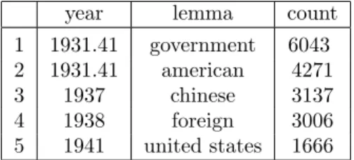
compound_nounsisTRUE,PrepTextidentifies compound nouns (ex: “Soviet Union”) and returns this string as one word instead of two. Overall, the PrepText function takes the longest time to run because it is computationally dense: stripping every word, tagging every word, removing stop words and combining compound nouns, counting up every lemma, and reporting its frequency. Individual documents no longer matter, but the number of times a word appeared inany document from a year is the new statistic of interest. In this sense, we can think of all of the documents relating to a year as the “text” from that year. The output of PrepTextmay look something like Table 1.2.

year lemma count 1 1931.41 government 6043 2 1931.41 american 4271 3 1937 chinese 3137 4 1938 foreign 3006 5 1941 united states 1666

Table 1.2: Example output fromPrepTextfunction

tf-idf and Adjacency Matrices An important question in translating text information into networks is how to decide edge weights and create the adjacency matrix. Weights, in this case, refer to how similar texts are to each other, which is an incredibly complex thing to calculate. Bail (2016) uses Term Frequency-Inverse Document Frequency (tf-idf) as this measure, to weight the connection between a term and a document. Term frequency is simply how many times a term appears in a document. Inverse document frequency, on the other hand, was proposed by (Jones, 1972), and is represented by idf(t) = ln( nd

nd(t)), in whicht is the

term we want to investigate, nd is the total number of documents and nd(t) is the number of documents

containing the term t (Silge & Robinson, 2017). By using natural log (ln), inverse document frequency puts more weight on “important” words3_{by decreasing the weight of words that appear commonly. Put all}

together,

tf-idf=tf(t)·idf(t)

tf-idf is commonly used in natural language processing tasks, including most search engines.

Intextnets,tf-idf is used to calculate weights for a sparse adjacency matrix for a text network between terms and documents (a ”bipartite” network). The function takes in a prepped data.frame, as shown in Table 1.2. In the calculation oftf-idf for this problem, the “term” is eachlemmaand the “frequency” is the number of times that lemma appears from all the words in the text from a year. In this case, the inverse document frequency refers to all of the words in the text of the year, and the log of the inverse proportion of the times the lemma appears in all the words.4 _{On the computational side, the function} _{bind_tf_idf}_,

part of theRpackagetidytext, calculatestf-idf values used intextnets. Then,textnetscreates a sparse adjacency matrix using thecast_sparse function, also in tidytext. Ultimately, the adjacency matrix of the network between documents is a one-mode projection of the tf-idf values onto the network (Silge & Robinson, 2016; Bail, 2016).

3_{In this case, importance is specified by a word being more rare. The idea is that if a word occurs a lot, it is probably a}

word that does not add much meaning.

4_{It is important to note the different uses of the word “document” in this thesis:}_FRUS_{has many individual documents and}

(12)

Creating and Visualizing Text Networks

Once thePrepTextfunction runs, creating and visualizing the text network is very simple.

1 # C r e a t e T e x t N e t w o r k

2 c o u n t r y _ n e t w o r k < < - C r e a t e T e x t n e t ( t e x t s _ P r e p p e d )

3

4 # S e t a s e e d a n d s a v e a p i c t u r e

5 set . s e e d ( 8 8 )

6 v i s n e t < < - V i s T e x t N e t ( c o u n t r y _ network , a l p h a = 0.25 , l a b e l _ d e g r e e _ cut = 0)

7 g g s a v e ( p a s t e ( c o u n t r y _ name ," . jpg ") , v i s n e t )

8

9 # V I P S T E P : S A V E T H E R E N V I R O N M E N T F I L E

10 s a v e . i m a g e ( f i l e = p a s t e ( c o u n t r y _ name , " . R D a t a ") )

set.seedsets the randomization seed for how the visualization will look. The alpha variable is a “tuning parameter.” For example, ifalpha= 0.25, all edges beyond the 75th percentile (1−0.25 = 0.75) for strength will be removed. The importance of this parameter is so that we can visualize the important structure of the network, not the “hairball” that comes from including too many edges. An example is in Figure 1.2.

(a) (b) (c)

Figure 1.2: Change inalphalevel for China text network. (a)alpha= 0.75; (b)alpha= 0.50; (c)alpha= 0.25

Discovering Trends and Characteristics

The last feature oftextnetsis identifying trends and characteristics through standard mathematical network theory models. Three main statistics used in network theory are community detection, modularity, and centrality. In this project, I only used the centrality measure.

Betweenness Centrality Betweenness centrality is one of the most important statistics in network theory. It was first proposed in Freeman (1977). It represents how central a node is to the overall network by calculatingshortest paths, the fastest or easiest way mathematically to get from one node to another node. The formula is:

bi= X

s6=v6=t∈V

σst(v)

σst

,

wherebiis the betweenness centrality withσst representing the total number of shortest paths from nodes

to nodet andσst(v) representing the total number of shortest paths fromttosthat pass through nodev.

(13)

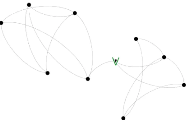
Figure 1.3: A bi-community network with node V having a high betweenness centrality

(14)

2

Data Collection

InFRUS, volumes have subtitles with the names of countries or areas of the world to which documents refer. With a dataset of more than 400,000 total pages, I decided to start my investigation by splitting up the pages into sets including any document in which a country is written about. I then created text networks, using

textnetsfor each country, withV being all years in which the documents occurred andEbeing calculated bytextnetsthroughtf-idf-created adjacency matrices, discussed in 1.2.1.

2.1 Separating Dataset into Individual Countries

I debated whether I thought manually separating the pages or coding a program to separate the pages would be both more efficient and precise. Eventually, I settled on a method of manual separation that used Excel’s search features due to potential detection issues with simple coding programs, such as identifying documents with the name of a country that did not actually refer to that country. Almost all searching happened in thetitlecolumn, since these fields usually include the name of the document and the country or region for which the document refers.

My method started with removing all pages with certain titles that indicated that they did not contain documents. These included:

• Delete all completely blank rows

• Delete all rows with titles that include “[Title page]” • Delete all rows with titles that include “[Cover]”

• Delete rows with titles that include “Index” and are not appendices • Delete all rows with titles that include “[Half-title]”

• Delete all rows with titles that include “[Contents]”

I also did not include any Prefaces, List of Persons, or other lists in the country subsets.

I then went through each country in the dataset, working from the FRUS website. I first searched the name of the country in thetitlecolumn and then manually scrolled through each row to actually determine if the document belonged in the country’s subset. If it did, I copied it to a separate Excel document for that subset.

In the next sections, I will illustrate some examples of countries for which creating subsets involved larger logistical and philosophical decisions.

2.1.1 Countries with Changing Names

(15)

Table 2.1: Example search terms to create subsets

country subset search terms example title

Turkey “Turkey”; “Turkish Empire” FRUS: Foreign relations of the United States, 1946. The Near East and Africa: Turkey

Table 2.2: Example search terms to create subsets for multiple names country subset possible names

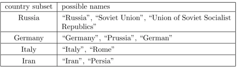
Russia “Russia”, “Soviet Union”, “Union of Soviet Socialist Republics”

Germany “Germany”, “Prussia”, “German” Italy “Italy”, “Rome”

Iran “Iran”, “Persia”

Additionally, some countries became nations during this time period (examples include Czechoslovakia and Australia). For these new countries, the subsets only begin once the United States acknowledges their existence inFRUS titles.

2.1.2 Countries with Changing Boundaries

Another logistical decision related to countries for which boundaries changed over the 100 year time period, or even those that still contain land disputes. A good example of this is Israel. Israel was created in 1948, causing an ongoing conflict with Palestinians in the region (Foreign Relations of the United States, 1948). Although this issue is highly political, Palestine is currently under Israeli control, so the search term “Palestine” is combined with the subset “Israel.”

Another example in this dataset of this phenomenon is the United Kingdom, which officially became the United Kingdom of Great Britain and Northern Ireland in 1922 (Joyce & Briggs, 2019). Wales and Scotland, however, united with England in 1536 and 1707, respectively, forming the United Kingdom of Great Britain (Joyce & Briggs, 2019). Since Northern Ireland eventually became a part of the United Kingdom as it is today, even though it was not included until 1922, I included these documents in the Great Britain dataset. In actuality, due to the nature of FRUS document naming, documents did not exist with Ireland named before 1922. After 1922, documents refer to the “United Kingdom of Great Britain and Northern Ireland,” which, of course, belongs in this dataset.

Former Colonies

In the period from 1860-1960, many countries that were originally colonies gained independence. This connects with 2.1.1, since these countries effectively changed names over time through gaining independence. As a result, I subsetted documents based on the current country for the location to which that document refers. For instance, French Indochina was the colonial name referring to modern-day Vietnam, Laos, and Cambodia (Editors, 2019). All documents referring to French Indochina, then, belong in all of the subsets of Veitnam, Laos, and Cambodia.

2.1.3 Documents for Multiple Countries

(16)

2.2 Cleaning Network Data

After separating all datasets by hand using the methods discussed above in 2.1, I manually checked through documents to make sure that these documents actually referred to the subset country. One example is that many documents referring to China in the title actually talked about Japan, such asFurther Japanese

political and economic penetration into China, 1934-1936. I then removed these documents. In addition

to manually checking that documents referred to the subset country, I employed different computational functions to clean datasets on the sentence and word level.

Stop Words and Symbols

In textnets’ function PrepText, there is the option to remove stop words (Bail, 2016). Stop words are those words that occur frequently in language but do not add any meaning. Some examples include: “I”, “me”, “my”, “and”, “but”, “if”, “or”. If the option to remove stop words is set totrue,textnetsuses the

tidytext functionget_stop words. This function reads through each word in the dataset and identifies stop words via the Snowball stop words dataset. A list of all stop words included in this dataset can be found at Snowball stop words List (Porter, 2002).

Stop words are not the only parts of sentences that need to be removed to accurately create text networks and properly analyze results. Scraping from the Internet usually leaves text data with unwanted symbols and blank spaces. I used the packagetextclean’s functionstrip, which removes all symbols and numbers (Rinker, 2018). After usingstrip, I removed all blank rows and other symbols.

1 p r e p p e d _ 2 = t e x t s _ P r e p p e d

2

3 p r e p p e d _ 2 = p r e p p e d _ 2[ ! is . na ( p r e p p e d _ 2 $ l e m m a ) ,] 4

5 p r e p p e d _ 2 $ l e m m a = s t r i p ( p r e p p e d _ 2 $ l e m m a )

6

7 p r e p p e d _ 2 = p r e p p e d _ 2[ ! p r e p p e d _ 2 $ l e m m a == " ",] # r e m o v e a l l r o w s j u s t s t r i p p e d 8

9 # c l e a n a l l r o w s w i t h o n l y o n e l e t t e r in t h e m

10 p r e p p e d _ 2 = p r e p p e d _ 2[ ! s u b s t r i n g ( p r e p p e d _ 2 $ lemma , 2) == " ",]

11

12 p r e p p e d _ 2 = p r e p p e d _ 2[ ! p r e p p e d _ 2 $ l e m m a == " ’ s ",]

Removing stop words and generally cleaning the text is especially important in the kind of text analysis computed in this thesis, as similarities between years is calculated withtf-idf. Even thoughtf-idf lowers the weight of frequently occurring words, many instances of the word “and” would make the program believe that documents from different years are more similar than they actually are for practical purposes.

Words Referring to the Country Itself

It is important to remove all words that would appear often without adding practical value for analysis. Since these datasets contain all documents in which the State Department of the United States wrote about a country, logically, many or all years of documents referring to a country will contain words referring to that country or the people from that country. The inclusion of these words would, therefore, artificially calculate years as being more similar than they are practically. I removed alllemmaswith these terms. Table 2.3 lists some countries with examples of how varying lemmas could be in reference to the place or people. The logic explained in 2.1 applies here. A deeper explanation of why this process was necessary is explained in A.2. 1

1_{Note: Although the}_lemmas_{in Table 2.3 are uppercased, all words in the dataset are lowercase. This is forced through the}

(17)

Table 2.3: Examples of Country and Citizen Reference Lemmas

country subset lemma for references to country or citizens Afghanistan “Afghan”, “Afghanistan, “Afghanistani”

Chile “Chili”, “Chilean”, “Chile”, “Chilian”

Congo “Congo”, “Congolese”, “Kongo”, “Kongolese” Iran “Iran”, “Persia”

Russia “Russia”, “Russian”, “Soviet Union”, “Soviet”, “Russo”

Thailand “Thai”, “Thailand”, “Siamese”, “Siam”

United Kingdom “British”, “English”, “United Kingdom”, “Scottish”, “Scotland”, “Welsh”, “Brit”, “UK”, “Irish”, “Irishman”, “Ireland”

(18)

3

Findings

Once all documents were put into country subsets, the question became what use the data could give to researchers. Each subset was run throughtextnets, creating textnets, visualizing the results, and saving the resulting data. This was done, in the beginning, more as an exploratory exercise to see what might “appear” in the visualizations. Once all subsets were graphed, two big findings seemed to be true over all subsets: the presence of temporal patterns inVi,1 and the usefulness of betweenness centrality to communicate years

that are particularly “important” to that country’s history in relation to US foreign relations.

3.1 Temporal Nature of

V

i

Temporal data is that data which relates to time, or has time as part of its variability. Temporal data is extremely important in mathematical modeling because most data available in “scientific and statistical databases (SSDB)” has some relation to a time-stamp in which the data was created (Segev & Shoshani, 1987, p. 1). These types of data are often more meaningful when connected to a temporal variable, and sometimes do not even have a “current” version that would be meaningful (Segev & Shoshani, 1987). The

FRUS subset data is temporal because each document is connected to a volume year, or the set V with individual nodesvi,j, withi representing the subset number (referenced in B), andj representing the node

number in this dataset. Of course this data, then, would be temporal.

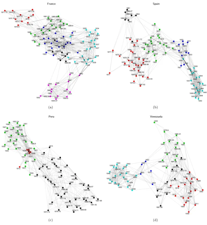
The interesting finding once the text networks were created, however, was that this temporal nature of the data greatly impacted the shapes of resulting text networks. All text networks created, no matter their size, approximately kept temporal data in date order. This means that, although nodes were not coded to space themselves by the date in which their node occurred, text data from the subsets matched dates that were close together as more similar, thus creating networks with years that were closer together in time as actually more similar quantitatively. This idea can be better understood through looking at a few of the resulting text networks from different size subsets as examples in Figure 3.1.2

Although these four networks have different orders, they all show approximate temporality in the placement of vertices. The similarity of nodes that are close in date can be shown beyond simple visualizations, however. The mathematical measurement for grouping nodes in a network is called community detection, which uses the descriptive statisticmodularity (Kolaczyk & Cs´ardi, 2014). Modularity refers to how dense edges are between nodes in a “cluster,” or “module,” versus the density between nodes outside of these groups. Mathematically, letCibe a candidate partition,fii =fii(C) is the fraction of edges connecting

Ci andCj, so that

mod(C) =

K X

k=1

[fkk(C)−fkk∗]2,

1_i_{represents the subset for a specific country, in alphabetical order from}_i_{= 1 to 93. These numbers are expanded in B.} 2_{Although all of the subsets in 3.1 are quite large, this pattern also follows for smaller subsets with orders as small as 6 or}

(19)

(a) (b)

(c) (d)

Figure 3.1: Networks showing nodes remaining in approximate temporal order, colored by modularity. (a) France,|V29|= 86; (b) Spain, |V77|= 81; (c) Peru,|V65|= 72; (d) Venezuela,|V91|= 64.

fkk∗ is the expected value of fkk in a model. fkk is usually defined as fk+f+k, where they are the row

and column sums of a K×K matrix with entries fij. (Newman & Girvan, 2004; Kolaczyk & Cs´ardi,

2014). Basically, modularity compares the number of edges expected for a node if the overall graph was randomized versus what is actually present in the graph. A graph with closely connected groups without many edges between nodes in other groups, then, will have high modularity. Modularity can be used for

(20)

a much-researched area in network science, and there are many ways to identify communities (Kolaczyk & Cs´ardi, 2014). textnets, though, uses the Louvain community detection algorithm to detect communities in text networks (Bail, 2016). Communities detected through the TextCommunitiesfunction intextnets, which utilizescluster louvain, shows which nodes are most similar to others and groups them. Louvian detection attempts to save processing power by not completing every possible combination for modularity. Since my networks are not too large, I decided to use cluster optimal from igraph instead (Csardi & Nepusz, 2006).3 _{This function tries all possible partitions and chooses the best ones. I ran}_{cluster optimal}

and the results further show how the subset text data’s temporal factor is a way to group nodes. It is important to note that I do acknowledge the problem of resolution parameters (Weir, Emmons, Gibson, Taylor, & Mucha, 2017). However, since the networks are small and I am focusing on proving temporality through modularity instead of investigating modularity itself, I do not need to worry about this issue.

As Figure 3.4 shows, years in their temporal order remain almost exclusively in discrete communities. The only exceptions are the few years that appear in a certain modularity class before the last year in the class before, but this almost always appears in one modularity class above or below, therefore making the overall nodes follow this generalization.

The importance in this finding is that the language inFRUS does, indeed, change over time. Although this may seem a bit trivial, this realization is actually quite significant. It means that, for all intents and purposes, any country that the United States discusses over time has changing information in its text data. Thinking about this historically, we can claim thatFRUS contains documents that represent a shifting view of countries, based on when, temporally, the document occurs.

3.2 Betweenness Centrality and Importance

Betweenness centrality, as defined in 1.2.1, describes how central a node is to a network’s structure overall. Due to the way that nodes in these subsets stay in temporal order in language similarity, we can make the claim that a node with high betweenness centrality is a year in which language significantly shifted. In other words, if a node (or, even a few nodes), occur at a “bottleneck”-shaped space in the graph, due to the temporal nature of these data, the nodes on one side of this high betweenness centrality node will approximately occurbeforethis node in time, and the nodes on the other side will occurafter.

textnets, as aforementioned in 1.2.1, usesigraph’sbetweennessfunction to calculate the betweenness centrality of each node (Bail, 2016; Csardi & Nepusz, 2006). The results of this calculation can, then, be used to scale node size in the visualization of text networks, using betweenness = TRUE in VisTextNet (Bail, 2016). The networks that were particularly interesting were those that had one node (or a small number of nodes) with a high betweenness centrality. These nodes were considered “important” for that country, since this year marks a significant change in language. The same four countries from above can be seen with

betweenness = TRUEin Figure 3.3.

Although these networks are exciting to see, simply looking at visualizations of text networks does not communicate anything about these important years compared to other nations.4 This method also does not show this data temporally, which is important for these data as documents over time.

3.2.1 Betweenness Centrality Measures as

y

With betweenness centrality measures for each country, measures of overall betweenness centrality could be calculated for the entire dataset. First, betweenness centrality measures for each year were collected for each country. The country was also tagged with a location variable, which signified the area of the world in which this country exists. The purpose oflocationis to allow analysis based on the area of the world, since I hypothesized that perhaps larger subsections of the world would be more responsive to betweenness centrality changes together than individual countries. To collect all betweenness centrality measures, I reran a modified

3_{In all}_textnet _{calculations, I replaced}_{cluster louvian} _with_{cluster optimal}_{. This means that my functions were not}

exactly the same astextnets, but since I was only using this option to show temporality, it made no impact on the overall results.

(21)

(a) (b)

(c) (d)

Figure 3.2: Years graphed by community. (a) France ; (b) Spain; (c) Peru; (d) Venezuela.

version of CreateTextnetwhich saved the betweenness centrality measures for the inputed .RData file, as well as updated this country’slocation.5

1 c a l c b c < - f u n c t i o n ( t e x t _ network , a l p h a = .25 , l a b e l _ d e g r e e _ cut =0 , b e t w e e n n e s s = FALSE ,

c o u n t r y n a m e , l o c a t i o n s ) {

2

3 # f u n c t i o n s f r o m o r i g i n a l C r e a t e T e x t n e t s . . . .

4

(22)

(a) (b)

(c) (d)

Figure 3.3: VisTextNet with betweenness centrality for node size. (a) France ; (b) Spain; (c) Peru; (d) Venezuela.

5 a l l b c 1 < < - d a t a . f r a m e ( y e a r = V ( p r u n e d ) $ n a m e )

6 a l l b c 1 $ bc < < - b e t w e e n n e s s ( p r u n e d )

7 a l l b c 1 $ c o u n t r y < < - p a s t e ( c o u n t r y n a m e ) 8 a l l b c 1 $ l o c a t i o n < < - p a s t e ( l o c a t i o n s )

9 }

10

11 # w r i t e a l l of t h e i n f o r m a t i o n t o g e t h e r i n t o a . c s v f i l e

(23)

13 w r i t e . csv ( allbc , " t o t a l_b e t w e e n e s s c e n t . csv ")

14 rm ( l i s t = s e t d i f f ( ls () , c (" a l l b c ", " c a l c b c ") ) ) # c l e a r s m e m o r y e x c e p t f o r t h e s e t w o f u n c t i o n s 15 gc ()

A list oflocationfor each country is in Table B.2. These locations were assigned based on where a standard Google search placed the country.

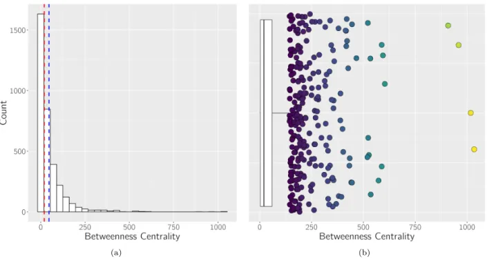
Only 81 countries out of 93 total had nodes with calculable betweenness centrality. The following table shows summary statistics on thebccolumn.

minimum Q1 median (M) mean (µ) Q3 maximum 0.00 3.00 20.00 46.69 59.00 1034.00

The difference between M and µsuggests a strong skew to the right in the distribution of betweenness centrality measures. This this further illustrated in the histogram of betweenness centrality, shown in Figure 3.4a.

(a) (b)

Figure 3.4: Betweenness centrality Distributions. (a) Histogram of betweenness centrality. µ = 46.69 (blue),M = 20 (red) ; (b) Boxplot with Outliers (jittered) for betweenness centrality.

Given the high number of outliers as well as the incredibly skewed distribution, analysis for betweenness centrality in these data is best calculated on the outliers only. A calculation of outliers involves the

Interquartile Range (IQR), calculated by

IQR=Q3−Q1

where Q3 and Q1 are the points that define quartiles I and III. Outliers are then defined as those points which lie beyond 1.5·IQRofQ1 orQ3. For this dataset,

IQR→59−3 = 56 1.5·IQR= 84

(24)

All betweenness centrality measures above 143 are outliers and were included in the new dataset. This new subset has the following summary statistics:

minimum Q1 median mean Q3 maximum 144.00 169.00 200.00 253.86 289.00 1034.00

To investigate this data visually, Figure 3.5 shows the top two nodes from each country in the outlier dataset.

Figure 3.5: Top Two Nodes for Each Country in Outlier Dataset graphed over time by betweenness centrality, colored by location

Interestingly, only 45 countries out of 81 in the original file have outlier nodes. The outlier set is heavily European countries, as shown by Figure 3.7a.

Smoothed Data

Since many countries in this dataset have either nonexistent betweenness centralities for certain years, for which zeroes are inputted, or many zeros as actual values for betweenness centrality, the data in its original form is “choppy” and difficult to analyze accurately. One method used for accommodating for data with a lot of noise is to smooth with a window filter. There are many types of smoothing windows, including the Gaussian function, also known as the probability density function of the normal distribution (Weisstein, 2019). The equation for this famous curve is:

f(x) = 1

σ√2πe

(25)

We can use the Gaussian function to create a window function, which smooths data by fitting it with the Gaussian function. An example of the Gaussian window function can be found in Roy and Morshed (2013, p. 3).

WG(n) =e−

1 2(

n−(N−1)/2

σ(N−1)/2 ) 2

,

where, “–N/2 ≤ n ≤N/2, σ ≥ 2 is the tuning parameter of the window to have the desired “main lobe width – side lobe peak” trade-off and window length is M = N+ 1.” R has a package, smoother, which takes in data and returns it after it has been smoothed (Hamilton, 2015). The Gaussian smoothing function is calledsmth.gaussian. The standard function assumes asmoother.windowsize of 0.1, or 10% of the data to smooth.

1 s m t h . g a u s s i a n ( x = s t o p (" N u m e r i c V e c t o r ’x ’ is R e q u i r e d ") , w i n d o w = g e t O p t i o n (" s m o o t h e r . w i n d o w ") , a l p h a = g e t O p t i o n (" s m o o t h e r . g a u s s i a n w i n d o w . a l p h a ") , ... , t a i l s = g e t O p t i o n (" s m o o t h e r . t a i l s ") )

The window size is the most inconvenient part of using a smoothing method. The window size determines the width of the data that is smoothed at any given point. As a result, smoothing the year data results in “lost” information about the first four and last five years (1861, 1863, 1864, 1865.66, 1950, 1951, 1952.54, 1955.57, and 1958.6). As a result, after smoothing, we cannot make conclusions about the post-World War II era, and especially not for the early Cold War. Although it is messy, Figure 3.6 shows what the betweenness centrality data looked like after it was smoothed.

Figure 3.6: Smoothed Betweenness Centrality Data by Country, colored by location

(26)

IQRsm →28.97−0 = 28.97

1.5·IQRsm = 43.46

Q3sm+ 43.46 = 72.42

The outlier data for the smoothed data was, in many ways, similar to the unsmoothed set (which was intentional). There are small differences in the proportion of outlier nodes in the smoothed dataset from different locations, however (see Figure 3.7). For instance, the bottom four locations for location (Africa, Balkans, Eastern Europe, and Scandinavia) all switched ranks for proportion. Other than this difference, however, the proportions remained similar over the two sets.

(a) (b)

Figure 3.7: Pie Chart of Proportion of Outlier Nodes by Location. (a) Original; (b) smoothed by Gaussian window function.

In looking at Figure 3.6, there appeared to be consistent peaks and troughs over many locations. This speaks to an idea of historical periods. It also seemed that the highest nodes for each year, connected by a line of highest betweenness centrality, would communicate the most information about when historical periods occur overall. When the outlier betweenness centralities for the smoothed data was graphed, definite peaks for betweenness centrality “height” became contrasted with troughs of particularly “small” betweenness centrality (Figure 3.8). Due to using Gaussian smoothing, most of the highest peaks are dominated by nodes from one country. It is important to note, however, that most peaks have more outliers from the same location also peaking, albeit to a smaller extent, in a similar range of dates. This suggests the importance of locality for impactful historical events.

The next step is calculating historical time periods. When looking at individual countries, a higher betweenness centrality statistic explained about this node’s location in the network and, thus, told of its resulting importance. When using all betweenness centrality measures together, however, interest lies in smaller betweenness centrality “troughs” and higher betweenness centrality “peaks.” There are also times that are, on average, low change periods, versus the big peaks that stand out visually. With many countries, I am making a system-wide argument, which necessarily differs from the method used for individual countries. In Figure 3.8, historical periods can be seen when looking at where the curves begin to increase in slope, thus showing acoming change in events. This is a time-period “build-up.” We can define a historical time period, then, as the distance between local minima (or, local points where events begin to build). This follows with the notion that changes are precipitous, and influence a large amount of time.

(27)

Figure 3.8: Outliers with gray line connecting the top outlier for each year. Dotted lines connect the location’s top outlier for each year. Top outlier for each year labeled with its country.

Period 1 2 3 4 5 6 7 8

First Year 1872.73 1879.80 1890.91 1897 1919 1925 1938 1945

Table 3.1: Historical Periods

Of course, a few of these historical periods particularly stand out. 1897-1919 is clearly World War I, 1919-1925 is the in-between and reconstruction period, 1919-1925-1938 is the Great Depression, and 1938-1945 is World War II. The World War I period is the one that stands out the most visually. Also, the case could be made for 1) breaking the period up into two periods from 1897-1912 and 1912-1919 and 2) moving the beginning of this time period to closer to 1901 or 1902 because the slope from 1897-1902 is more gradual than after that point. This peculiarity speaks to the incredible historical importance of World War I as an event.6

3.3 Networks of Historical Periods

The logical next step after determining historical periods was to subset the data into the historical periods and rerun textnetson these subsets with the countries as the nodes instead of the years. Using the same ideas as before, the networks should show the similarities between years over a time period. My hypothesis was that countries from a similar location would be more likely to be in the same communities. Since these are split into the historical periods chosen before, it would make sense that events mentioned in these

6_{As mentioned before, due to smoothing, no conclusions can be drawn about the post-World War II period and no outliers}

(28)

Figure 3.9: Dotted lines defining important historical periods by betweenness centrality.

documents would already be similar based on the location throughout the world.

3.3.1 First Two Historical Periods

The communities detected bycluster optimalmostly follow the intuition about communities being related to the location of the country (see Tables 3.2 and 3.3). The actual networks also show a shape with clusters of countries with similarities between them over this time period.

The main reason to use textnets for these time periods was to try to find information difficult to discover using standard historical research methods. texnetscan pull out words that are significant to each community for the overall time period, for instance. Many of the words detected through this method were country or city names. An example is the lemma “abyssinian” for community 2. This refers to the conflict between Egypt and, eventually, Italy against Ethiopia (once called Abyssinia) (Erlich, 2007). This conflict would end up involving many proxy nations, including Russia. It is possible that the United States cared about this conflict, at least in part, because this area involved a famous United Kingdom rescue mission of Europeans from the Ethiopian highlands in 1867-1868. (Matthies & Rendall, 2012). The second highest group of “important” words in the communities, however, were names of generals and leaders of countries. One example is the lemma “colonel latorre” for community 4 in the 1872-1890 period. Colonel Latorre was the president of Uruguay from March 1876-March 1880 (L´opez-Alves, 2000, p. 72). He is credited with being one of the first “state-makers” for Uruguay (L´opez-Alves, 2000, p. 92).

(29)

(a) (b)

Figure 3.10: Two historical period networks. (a) 1872-73-1879-80 period; (b) 1879-90-1890-91 period.

1 2 3 4

Argentina Austria Denmark Paraguay Belgium Egypt France Uruguay Bolivia Hungary Germany Venezuela Brazil Liberia Greece

Chile Morocco Italy China Russia Norway Colombia Tunisia Sweden Ecuador Turkey Switz. Haiti

Japan Mexico Peru Portugal Spain Thailand UK

Table 3.2: Communities by modularity for the first historical period.

1 2 3 4

Argentina Austria Chile China Colombia Hungary Peru Italy

Denmark Japan

El Salvador Korea

France Portugal

Germany Russia

Greece Haiti Liberia Mexico Spain Switz. Thailand Turkey UK Venezuela

(30)

Period 1 2 3 4 5 6 7 8 9 1st Year 1872.73 1879.80 1890.91 1897 1912 1919 1925 1938 1945 Pages 1282 834 3672 15957 8816 10255 31071 45551 28911

Table 3.4: Periods and Pages Included

3.3.2 Surprising Findings

Unfortunately, this method did not produce the same results for the historical time periods with larger texts. The time periods steadily increased in document number as time increased, as is shown in Table 3.4. This is not surprising, since advancements in technology as well as the growing interconnectedness of the world led to more documents being created.

The results from creating networks of the time periods with more pages, however, seems to show that

textnets cannot differentiate meaningful information withtoo many documents, while also having nodes with small amounts of text. The networks in Figure 3.11 do not make logical sense. The 1897-1912 period seems to have no form at all, with all countries connected to each other without distinguishing characteristics. San Marino, Greece, and Tanzania are central in the 1925-1938 period. The fact that Congo, San Marino, Greece, and Tanzania stand out in two of these networks suggests the potential problem. All of these countries have disproportionately small amounts of documents compared to other countries. It seems highly likely that too much data for some countries and too little data for others has muted individual, and meaningful, information from presenting itself. Instead, countries are connected to the smallest subsets because, perhaps, thelemmasfrom these groups have relatively large term frequency, and thus, highertf-idf.

Let’s look at the 1912-1919 period, for instance. In this network, “Congo” is the most central node. As this period represents the most significant historical event of modern time, World War I, the fact that Congo is most central clearly does not make sense. The reasons for why this is happening can be found in the calculatedtf-idf values for eachlemma in the full set. Once the values are computed andlemmas used by only one author are removed, a data.frame with each lemma and computedtf-idf value remains. Table 3.5 shows thelemma, group (country) thislemmabelongs in, the times thislemmaappears, and the resulting computed tf, idf, andtf-idf. Five of the top 20, and 4 of the top 4,tf-idf values correspond to alemmafrom Congo.7 _{The counts of these}

lemmasare all either 1 or 2. In turns out that all of these lemmasare in one document, written in 1916. It reads:

KONGO[:] ABROGATION BY THE UNITED STATES OP ARTICLE 5 OP THE TREATY OF JANUARY 24, 1891, CONCLUDED BETWEEN THE UNITED STATES AND THE INDEPENDENT STATE OP THE KONGO.—ACCEPTANCE OP THE ABROGATION AND DENUNCIATION OP THE TREATY BY BELGIUM. (See Belgium)8 ₍_{Foreign Relations of the}

United States, 1916)

Having only this one document represent all of the data for this country, then, incredibly inflates the tf-idf values for these lemmas. The network adjacency matrix is defined as the cross product of the sparse

tf-idf matrix. This means that the weights between countries are defined as the sums of multipliedtf-idf

values when two countries have the same lemma. Since Congo has so few words available, its lemmas have disproportionately high tf-idf, as aforementioned. This means that the weights between Congo and other countries will get a “boost” compared to other countries. These other countries, whose lemmashave much smallertf-idf values, need many more overlapping words to get to the same added weights on their edges. Table 3.6 shows the weights added to the edges between Congo and the various countries listed. Although these numbers are small on the absolute scale, the added weights, especially for Belgium, Bolivia, Hungary, Austria, and Morocco, are large compared to the kinds of weight additions expected by only five possible overlapping lemmas. Unsurprisingly, these countries with high edge weights are the ones closely connected to Congo in the network visualization.

7_{The 4th}_lemma_{, belgium, shows why I did not remove the names of countries from these historical period text networks.}

Although many of the toptf-idf values are for proper nouns referring to its own country, the ones that are proper nouns and refer to a different country create an appropriate connection between countries that should be reflected in the network.

(31)

(a) (b)

(c)

(32)

Number Group lemma Count tf idf tf idf 1 Congo united states op article 1 0.05 3.157 0.158

2 Congo kongo 1 0.05 2.464 0.123

3 Congo abrogation 2 0.1 0.906 0.091

4 Congo belgium 2 0.1 0.806 0.081

5 Iran shah 5 0.027 2.241 0.061

6 Iran coronation 4 0.022 2.752 0.059

7 Congo denunciation 1 0.05 1.142 0.057

8 Finland finnish 340 0.02 2.752 0.055

9 Finland finland 440 0.026 2.058 0.053

10 Bulgaria bulgarian 41 0.021 2.464 0.052

11 Iran teheran 3 0.016 3.157 0.051

12 Bolivia bolivia 33 0.027 1.548 0.042

13 Ukraine ukraine 156 0.015 2.752 0.041

14 Ukraine ukrainian 156 0.015 2.752 0.041

15 Switzerland swiss 30 0.018 2.241 0.04

16 Norway spitzbergen 26 0.01 3.157 0.032

17 Romania roumania 9 0.023 1.365 0.032

18 Paraguay paraguay 76 0.016 1.904 0.031

19 Denmark danish 1179 0.018 1.771 0.031

20 Colombia colombia 592 0.025 1.211 0.03

Table 3.5: Top 20tf-idf values forlemmain 1912-1919 historical period.

Country Weight Added Country Weight Added

Belgium 0.0017 Italy 7.78E-06

Bolivia 0.00054 Finland 7.65E-06 Hungary 0.00047 Ecuador 6.76E-06 Austria 0.00047 China 6.71E-06 Morocco 0.00012 Haiti 6.59E-06 Germany 8.94E-05 Ukraine 6.15E-06 Greece 7.20E-05 Japan 4.09E-06 Turkey 6.16E-05 Mexico 3.52E-06 Netherlands 4.07E-05 Denmark 3.15E-06

Peru 3.10E-05 Russia 2.87E-06

Honduras 1.96E-05 Colombia 2.72E-06 Brazil 1.69E-05 Panama 2.65E-06 United Kingdon 1.60E-05 Nicaragua 1.32E-06 France 1.45E-05

Table 3.6: Weight added to edges of countries listed by the top 5

lemmasfrom the Congo group. In addition to the problems with

Congo, a similar instance occurs for Iran, which also has a very small number of words available compared to other countries. As a result, both Congo and Iran are featured centrally for the text networks created. If any other country has the same lemma, textnetsassumes that it must be very similar since each

lemmais marked as being very important to these small text countries. This is clearly also the phenomenon occurring with Tanzania, Greece, and San Marino featuring as central in the 1925-1938 time period.

tf-idf can skew importance

calculations when there are too few

words available. When some nodes represent text of very long length and some others represent texts of very short

length, meaningful information is lost. In data science, usually more data is better to make models. Too much variability in the lengths of texts, however, can create noise that muddies the results. That seems to be the case for these later historical periods. One possible solution could be to remove the countries with lower-boundary outliers in terms of the size of the text. Perhaps this would put more emphasis on the countries the United States discussed the most. It is also possible, however, that the current version of

(33)

3.3.3 tf-idf

and Big Data

As mentioned previously,tf-idf puts more weight on uncommon words through the use of natural log (ln). This research has shown a potential issue withtf-idf, however. This thesis contained data sets with large and small text sets together, which caused a loss of meaningful information. There may also be a problem with

tf-idf and text sets that are simplytoo large, however. It may be that ln is not strong enough to minimize the effects of common words, even after removing stop words. An example is shown in Appendix A, when I discuss the huge impacts of compound nouns in the update of textnets(A.1b). In that case, tf-idf could not minimize these names enough to show the meaningful information.

There may be a fundamental problem withtf-idf that is causing this issue. Althoughtf-idf is used widely in natural language processing and information retrieval problems, inverse document frequency (idf) was first proposed as a heuristic with little theoretical background (Jones, 1972; Robertson Stephen, 2004). Many scientists have since tried to calculate theoretical reasons why this definition of idf is the correct measure. Robertson Stephen (2004) goes through some various suggestions for theoretical bases. He explains, for instance, that one reason that a logarithmic function is better than a linear function is because a log allows for a probabilistic understanding of the accepted additive ideas of scoring functions in information retrieval theory. Stephen additionally shows thattf-idf works in the Okapi BM25 method, which tries to find a theme in a document. These documents must all beelite, which means that they all refer to a theme that can be determined. Using these examples, Stephen concludes that scientists generally know why tf-idf has been successful.

These justifications as to why idf, and thereforetf-idf, is a theoretically sound idea may make sense for information retrieval, but many applications natural language processing do not deal with text that is short (like a search query in information retrieval problems), but instead investigate vast amounts of text data. To test the limits oftf-idf on large datasets, I investigated the largest country subset, China. The China network had always seemed to be an outlier. It was the only country network without a clear temporal pattern, and it also seemed to be more of a hairball shape. After finding these recurring problems with

tf-idf, I wondered if the reason that this network looked different was because of the size of its text. I tested this hypothesis by setting up an experiment where I took the full dataset and took a random sampling of a certain percentage of documents within year. Using this method, I was able to keep the same distribution of documents over each year, but I also had smaller subsets of the documents. I made 9 subsets, increasing the percentage by 10% each time.

1 c h i n a 1 = c h i n a % >%

2 g r o u p _ by ( y e a r ) % >%

3 s a m p l e _ f r a c (.1 , r e p l a c e = F A L S E )

I then ran each of these subsets through the exact same process as the other text networks to create the visualizations. The results confirmed my hypothesis. As the size of the texts increased, the network showed less meaningful information. Basically, the more documents were included, the less any individual year mattered to the structure of the network. The contrast between the network created by 10% of the available documents and the full set, shown in Figure 3.12, is stark. In the small network, the nodes follow the temporal pattern, whereas the full set looks more like a hairball with no clear shape. It seems that at around the 30% mark, information starts to disappear, and by 50% of the documents, most meaningful information is hard to see (Figure 3.14).

This problem is not just represented in the visualization of the networks themselves. It appears that a shrinking of the average value oftf-idf is at the heart of this visual problem. I stripped thetf-idf values for alllemmas according to the codetextnetsuses to form the adjacency matrices.9 _{I then used graphed the}

data with boxplots to see if there were distinguishable differences between the distributions of the smallest subsets and the bigger subsets. Figure 3.13 shows that there are, actually, statistically significant differences in the distributions of the smallest and biggest subsets. Even though the bigger subsets have the largest absolutetf-idf values (Figure 3.13a), the distributions shrink closer and closer to 0 as the documents increase. Interestingly, this shrink almost looks like an inverse exponential function, perhapsy= 1_x, which would make sense due to the use of log intf-idf. This small experiment visualizes how, if x is the amount of text processed,

9_{The number of}_lemmas_{investigated in this test is 3,855,864. For reference, that is 3.56 times as many words as the entire}

(34)

(a) (b)

Figure 3.12: Smallest China subset compared with the full network. (a) 10% of documents,n= 3972; (b) full set,n= 39738.

(a) (b)

Figure 3.13: Boxplots of tf-idf for lemmas in subsets of increasing percentages of the China subset. (a) Completely zoomed out; (b) Y-axis limit set to .0006

lim

x→∞tf ·idf(x) = 0

(35)

(a) (b)

(c) (d)

(36)

4

Conclusions

History doesn’t repeat itself, but it often rhymes.

– Mark Twain

4.1 Importance of Study

4.1.1 Traditional View of Historical Periods

In historical education and discussion, it is common to see events referred to with note to their “period”. In reality, the definitions of historical periods and eras are incredibly variable and, in many cases, largely unknown. As Webster (2004, p. 47, 49) explains, all historical periods are ultimately representations and constructions of the researcher’s view of events, used to make sense of large amounts of information. This is true of qualitative subjects in general, as there is ultimately some level of arbitrary nature for claiming that one era starts somewhere and ends somewhere else. As Webster (2004, p. 48) writes,

Issues of periodization altogether have been little discussed either by general historians or by musicologists during the last quarter-century. This inhibition has multiple causes: the apparently simplistic, over-generalizing character of most period designations, the desire for objectivity in historical writing following World War II, the preference for ‘thickly textured’ history and cultural studies as opposed to the traditional ‘grand narratives’, the attractions of metahistory and the anti-foundationalist orientation of postmodernism.

As implied by this quote, there is little quantitative research in the subject matter of historical periods in modern history.

There is a problem with this ambiguity, of course, as both historians and researchers from other disciplines may refer to different years when discussing a time period in history. This is particularly problematic in fields like archeology which require a standard to categorize found items in the right time period. Doerr, Kritsotaki, and Stead (2008) have the most solidified proposal for how to name a historical time period. They suggest a computer-science based theory for naming archaeological time periods to standardize historical conservation and museum curator efforts. According to their research, the historical periods discussed in this paper are “cultural periods:” those that represent when a group of people’s ideas of the world change together. Cultural periods, due to the gradual way that ideas transform, often overlap and are incredibly difficult to pinpoint to a certain range of time. For reasons of practicality, cultural periods should, therefore, be associated with “indicators” of a change. This could be a new government type, event like a war, or new innovation (Doerr et al., 2008, p. 3). Although this still leads to some potential for disagreement, proposing cultural periods as defined by one major event, thought, or invention, allows for a focus that is unattainable otherwise.

4.1.2 American Cultural Time Periods: A Quantitative Step

The research outlined in this thesis introduces a new, largely unbiased way to detect cultural time periods.

(37)

by hand. The massive amounts of text available in these volumes, however, give a glimpse into the thoughts of American foreign relations officers and offices over 100 years. There is no better way to detect changing historical ideas and views than to investigate when people, living and working in the time period, began to change the way they discussed certain countries. This research method directly follows the concept of cultural time periods. Usingtextnets, mathematical network theory, and betweenness centrality, we have uncovered a means to suggest historical time periods from 1872-1949 from a United States perspective. Although this research applies only from the view of the United States, the results contribute a new theory of discussing and proposing cultural time periods.

4.2 Future Research Expansion

4.2.1 FRUS

: A Growing Body of Research

The FRUS documents used in this study were the ones digitized by the University of Wisconsin-Madison libraries and available online on their site. I used these documents because they were all completed by the same group and have had relatively little attention. Although the FRUS volumes began with President Abraham Lincoln, they technically will encompass each president’s term from 1861 on. The problem with using many of these volumes together, as with any classified government documents, is that the declassification and digitization process is incredibly slow. Today, volumes are available, and almost completed, through President Jimmy Carter’s term ending in 1980 athttps://history.state.gov/ historicaldocuments. Of course, this gives the possibility for expansion of this project by 20 years of documents now, with the assumption that there will be many more documents in the future.

The years now available that are not included in this study, 1960–1980, are incredibly important historically to United States/Middle East relations, as well as the beginning of the Cold War. Since these volumes are published quite slowly (for example, only five volumes are planned for declassification in 2020), it is possible to incorporate new data into the model and recalculate as information is released. Using this method, the findings explained in this thesis can continue to improve and evolve.

4.2.2 tf-idf

and Better Natural Language Processing

As is discussed in 3.3.3, tf-idf may not be the best method for natural language processing methods on large datasets. There have been suggestions for how to best improve this metric, including (Xia & Chai, 2011). As quantitative methods keep evolving in traditionally qualitative fields, more research is needed to solve the problems of tf-idf becoming less helpful as documents increase. Although ln is accepted for its convenient overlap with probability theory, perhaps a more powerful function with a power could better minimize the effects of too much text muddying the data. Perhaps the answer does not lie in a different method for assigning text statistics, but instead in a different, and better, method of cleaning the data in the beginning. It is possible that use of emerging machine learning techniques, like neural networks, could be used to pick out data that would be useful to show patterns in the first place. It would be important to remember if using this method, however, that one of the stated goals of using this quantitative methodology is to discover things that were not realized before. It would be tremendously important, therefore, to make sure that the user was not using a model to “discover” things they already knew to be true, rather than letting the computer tell them new information.

4.2.3 History is (kind-of ) a Cycle: Potential for a Prediction Model

With the introduction of advanced machine learning techniques such as neural networks, there is a push for improved event detection (ED). Many of these event detection tasks are designed to scrape websites and notice events in text such as those found in newspapers. Some examples of emerging techniques include Nguyen and Grishman (2016); Feng, Qin, and Liu (2018); Lei, Wu, Zhang, and Liu (2005).These techniques are still being created, butFRUS presents a dataset that could prove rich with events to find.

(38)