2017_Castro.pdf

(1)

Abstract

(2)

Acknowledgments

(3)

1 Introduction

Collateralized debt obligations (CDOs) are a type of asset-backed security, which have con-tinued to grow in popularity since the early 2000’s. First issued in 1987, the CDO is a relatively new financial instrument; as such, it has not been deeply studied and is still an area of undeveloped research. Contrary to equity instruments, a CDO is a fixed-income instrument, which assembles cash flows of names into layered groups of risk. These groups, known as tranches, act to lower risk through diversification of debt. CDOs provide numerous benefits besides lower risk, such as the ability to convert debt into capital, provide a larger market for fixed income investment, and offer a higher return of investment. With these attractive options, the CDO market grew from 69 billion in 2000 to 500 billion in 2006, a 620% increase. This growth continued until the 2007 sub-prime mortgage crisis, which was shortly followed by the 2008 global recession.

Credit derivatives are of particular interest due to the recent credit crises, a period with low issuance of credit. Usually, a credit crisis is a tightening of loans due to high failure in the credit market. Due to the difficulty in acquiring data on credit derivatives, indices are commonly used as a proxy for the market. The market share of these instruments varies over time, but consistently composes a majority. As such, they act as a well-fitted representation in order to study the events which cause high failure. By understanding the factors that drive this connectedness, the groundwork is laid for developing models which aim to predict, and possibly prevent, credit crises.

(4)

asset risk and overall portfolio risk. That is, these expectations of risk are partially a function of connectedness. This approach does not aim to calculate an individual investor’s risk, but instead the network formed by many such individuals. As such, networks are the result of the aggregate of investors’ expectations. Take, for example, news that a financial firm with a credit default swap may crash. When an investor hears this news, he/she takes into consideration the risk of his/her portfolio, including a consideration of how this crash may affect other assets. Right away, we can see this consideration has formed a network of the original firm’s CDS to other assets.

This contributes to a growing body of literature that applies networks to economics. Networks are not exclusive in financial markets or even economics, as they are applicable, but not limited to, game theory, evolutionary biology, and social media. However, their study and development is new to the field of economics, so difficulty arises in constructing a network, as it has no inherent measure that can be gathered by studying investors. By adding in a large data set of events, the connectedness measure is further developed as a tool for understanding the network, despite its open-ended interpretation. We start with an approach discussed in Diebold and Yilmaz (2015a) of connectedness being part of credit risk and portfolio choice before expanding further to event studies. We find that each sector has specific factors which affect it, with some factors being unique to the sector. Additionally, returns are sensitive to firm specific factors, while volatilities are sensitive to some firm specific factors and macroeconomic factors.

(5)

Section 6 presents the empirical model. Section 7 provides information on the data. Section 9 concludes the paper and reviews results and contributions.

2 Background

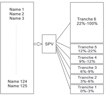
Before examining the role of CDOs in crises and the tools used to evaluate their risk, we must first understand their operation. A CDO begins when a special purpose vehicle (SPV), a specialized legal entity, aggregates the names1 _{into a CDO. Each tranche from this} aggre-gation process is given a rating by common credit rating agencies. Unlike stocks or bonds, CDOs do not have a direct market where investors post bids and asks. Instead, they are a contractual obligation between an issuer and an investor developed through a series of private communications. Cash flows of principal and interest payments are directed into the tranches in order of decreasing seniority, with the highest senior tranche having the least risk. As a result, coupon payments are inversely related to tranche seniority. Let us take, for example, a CDO sliced into six tranches. The highest tranche is known as a “senior” or “super senior,” whereas the lower tranches are “junior” or “mezzanine.” The lowest tranche of all is called an “equity” tranche, and it has the highest risk of loss. Each tranche has a percent spread of N-M percent, where N is known as the “attachment point” and M as the “detachment point.” For the purposes of this example, we will assign the tranches, in order of increasing seniority, 0-3, 3-7, 7-10, 10-15, 15-30, 30-100 percent. If a name defaults, the equity tranche will absorb all losses up to 3 percent of the total notional value (detachment point). This absorption will continue up the rank of seniority until the senior tranche stops receiving cash flows. When credit losses exceed the percent of the tranche, the entire amount for the investor is eliminated, and the investor loses his/her principal, and coupon payments will cease.

(6)

insurer for some fixed amount of time. The remaining principal is paid to the buyer by the insurer if the debtor defaults. In this way, the underlying asset(s) is insured against default by a credit default swap. Once the CDS contracts are defined, an SPV can create a synthetic CDO. A synthetic CDO is similar to a CDO, except the underlying assets are credit default swaps.

With the financial instruments underlying this study well defined, we can now discuss the issues of data and use of indices. First, data on collateralized debt obligation are quite hard to procure. As there is no market, pricing information is hidden in contracts and com-munications between investors and issuers. The underlying names, which are of particular interest, are so vast, that investors do not know their specifications. Rather, only the rat-ing information is known to them. For these reasons, several indices have been created to monitor and study the market indirectly. In this study, we use the CDX North American Investment Grade Index and the CDX North American High Yield Index. Both indices fea-ture the top 125 liquid companies on a rolling six-month basis. These two indices are also of particular interest as they have index CDO tranches issued, tie to the CDX index. As opposed to CDOs, these CDX.HY and CDX.IG indices function as synthetic collateralized debt obligations. Despite this, they function well as a proxy for the credit market. Several studies have found that the ratio of risk premium to the credit risk component is constant (Pan and Singleton 2008, and Longstaff et al. 2011). Given this analysis only takes into account the ordinal properties of the connectedness estimation, there are no issues with the use of spreads as proxies.

3 Literature Review

(7)

began when Li (2000) introduced a pricing model using a copula coefficient, which grew rapidly in popularity among financial markets. However, the incorrect use of this model has been cited as a major contributor of the sub-prime mortgage crisis (Duffie, Saita, and Wang 2007). In terms of a network, the underlying connectedness of CDOs begins in the pricing model, which takes into account a copula coefficient2_{. Many investment banks now} focus heavily on developing better models for the credit market, which differ heavily from the equity market in terms of accuracy and depth of knowledge. For studying the effect of events, in an aim to predict prices, Longstaff and Rajan (2008) examined a three-factor model, each factor being a firm failure, failure of multiple firms, or wide scale failure. Although they found that multiple factors were needed to better account for pricing using a Poisson process, they also found the current market to be efficient in its pricing of overall portfolios.

More recently, literature has transitioned beyond pricing, examining the connectedness of sovereign CDOs and CDOs to other markets. Bostanci and Yilmaz (2015) applied the Diebold-Yilmaz connectedness index to sovereign credit default swaps for 38 countries be-tween 2009 and 2014. They found two clusters of indices, composed of developed and devel-oping countries. Within this, they determined emerging market countries were the dominant factor in sovereign credit risk shocks, while developed countries displayed less risk. Addition-ally, Fonseca and Gottschalk (2012) applied the Diebold-Yilmaz measure to firm-level CDS data from Asia-Pacific Markets, analyzing the relation between stocks and CDS spreads. They determined a discrepancy exists between the implied volatility at firm-level and the realized volatility at market-level.

(8)

As a result, factors, both observed and unobserved, affect connectedness. Thus far, the lit-erature has examined a few particular events, such as Bernanke’s speech during the financial crisis (Bostanci and Yilmaz 2015).

4 Theoretical Setup

We follow Modern Portfolio Theory (Markowitz 1952). We begin with a single period model, where an investor considers available credit default swaps available before making his/her investment decision, beginning with an expectation of risk. As a credit default swap is a contract, the market is less volatile, meaning an investor cannot trade assets as easily. In this sense, this greatly reduces the need for a multi-period model, as investor need not re-evaluate his/her position often.

We now consider a multi-period model, where the investor is able to again invest, due to more cash flows. Now, the network expectation is subject to change the impact of an event on an investor. As these markets are traded at high volumes, most investors are professional, meaning they have constant access to information. When an event occurs, an investor compares his/her expectation of the network to the current realization, and then changes his/her position depending on the difference between his/her expectation and the realization.

Let us denote the expected network as E(O). Let the expectation of risk be E(Ri) =

f(E(O), oi),whereoi are other factors. An investor places weightwi on each asset as a split

of his/her portfolio, wherePn

i wi = 1. We define the portfolio return variance as:

ψ2_p =X

i

w_i2ψ_i2+X

i

X

j

wiwjψiψjρij (4.1)

where ψ is the standard deviation for the periodic returns of the asset, and ρij is the

(9)

ψρ=

q

ψ2

ρ (4.2)

Investors then choose a budget setB(p,f), given available funds f as:

B(p,f) = {x∈_R₊n :p·x≤f}, (4.3)

where p is the price vector for the CDS’s and x is an vector of volumes for the CDS’s. Given limited funds f, an investor chooses to invest in CDSs which fit his/her expectation

of return. An investor considers both return volatility and expected risk when making an investment decision. Our main conclusion of this model is investors examine the given information and form an expected value of risk. When an exogenous shock occurs, investors change his/her expectation of risk. As such, the connectedness between CDOs for each company changes, affecting the overall network structure.

5 Connectedness

5.1 Network Theory and Analysis

A network N is a collection of N nodes (or vertices) and L edges. Intuitively, a network represents relationships between these objects (nodes) as edges. A network can be directed, meaning each pair of nodes can have at most 2 edges between them, or undirected, meaning two nodes share a single edge. Mathematically, a network is an adjacency matrix A = [aij],

where aij represents the edge from node i to node j. In an unweighted network, aij = 0

(10)

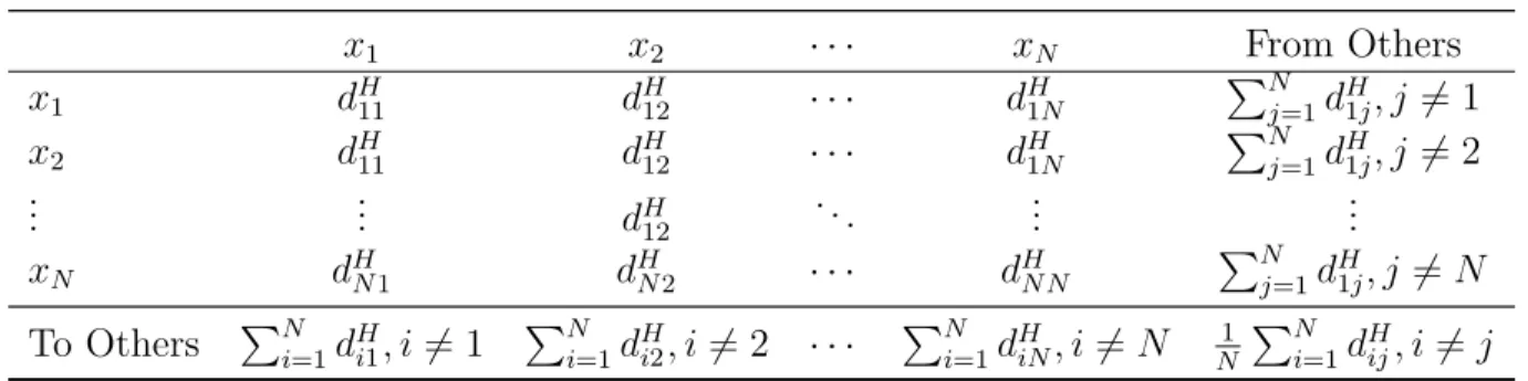
Network Theory is a relatively new area of study and tools to understand networks are still being developed. We begin with the connectedness table (Table 11.1), where the entries fromx1 to xN are analogous to the transpose adjacent matrix.

In estimating networks using variance decompositions, as discussed in the next section, we form N2 edge weights, where entry _θ

ij(H) gives the connectedness from node j to node

i. Networks are often large, dense datasets, which make gleaning useful information an impossible task. We can use several methodologies to gain useful information about a net-work, starting withnet connectedness. For a pair of nodes i,j we define pairwise directional connectedness as

C_iH_←_j =θij(H)

As Diebold and Yilmaz note, it is not necessarily true that C_iH_←_j = C_jH_←_i, so there are

N2−N pairwise edge weights. We then definenet pairwise directional connectedness as

C_ijH =C_jH_←_i−C_iH_←_j

Calculating the pairwise connectedness for all pairs allows a great degree of combinations for analysis. In similar convention, we examineto connectedness andfrom connectedness. To connectednessis the effect of a CDSito the system, which is high-yield and investment grade CDSs. From connectedness is the effect of the system to a CDSiof either index (we provide detailed calculations of connectedness in the following section). We can also calculate total directional connectedness from all others to i as

C_iH_←_•

N

X

j=1

j6=i

θij(H) (5.1)

Similarly, we can calculate total directional connectedness to all others from j as

C_•H_←_j

N

X

i=1

(11)

Differencing these two total measures gives us net total directional connectedness, which we will from here on refer to as just net connectedness, defined as:

C_iH =C_•H_← _i−C_iH_←_• (5.3)

Another aspect of interest in networks is communities, which are groups of nodes that are more densely connected among each other than other nodes. In this paper, we use the Louvain Method to detect communities (Blondel et al. 2008). This method has been used before with the Diebold-Yilmaz Connectedness Measure in Bostanci and Yilmaz (2015). The Louvain Method is an iterative process that maximizes modularity, a metric which measures how much more dense the detected community connections are compared to a random network. After detecting communities, we can examine which nodes (in this paper, companies or sectors) belong to the communities and the underlying features which drive their modularity.

5.2 Diebold-Yilmaz Connectedness Measure

We begin with N-dimensional VAR(p) model,

Yt=Φ1Yt−1+. . .+ΦpYt−p+εt (5.4)

where ε is white noise and Φ1, . . . ,Φp are coefficient matrices. Given the VAR(p)

process is causal and invertible, we can transform it to a MA(∞) representation Yt =

εt +A1εt−1 +A2εt−2 +. . . with N ×N matrices Ah. Now for a H-step ahead forecast

at timet, P(Yt+h|Yt, Yt−1, . . .) and for the corresponding forecast error

Yt+H −P(Yt+h|Yt, Yt−1, . . .) = εt+H +A1εt+H−1+A2εt+H−2+. . .+AH−1εt+1 (5.5)

We denote A0 ..=IN, the forecast error’s covariance matrix is Σe,H =

PH−1

h=0 AhΣεA0h, with

(12)

5.2.1 Cholesky Decomposition

We make use of the lower-triangular Cholesky factorLofΣε, i.e. the lower-triangular matrix

L with LL0 = Σε to decompose the forecast error variances. Using L, AhΣεA0h can be

written as (AhL)(AhL0), from which we have (AhΣεA0h)ii =

PN

j=1(AhL)2ij variable i’s

forecast error variance. Consequently, PH−1

h=0(AhL)2ij may be considered as the contribution

of (shocks to) variable j to variable i’s forecast error variance

5.2.2 Generalized Variance Decomposition

Cholesky decompositions are sensitive to ordering, so we may be reluctant to impose identi-fying assumptions; there are several ways to combat this sensitivity. One way, as in Diebold and Yilmaz (2009) is to take random permutations before the rotation and find the average, minimum, and maximum across these permutations. However, this was shown in Klößner and Wagner (2014) to underestimate the spillover index by up to a third.345 _{Additionally,} we can use generalized variance decompositions, which avoids using a rotation matrix, and thus does not impose identifying assumptions (although it has assumptions of its own). Gen-eralized variance decomposition (GVD) was introduced in Koop et al. (1996) and Pesaran and Shin (1998). To calculate it, we first measure pairwise directional connectedness, which measures the effect of company i on company j. This H-step-ahead generalized forecast error variance is given as:

θ(H) = σ

−1

jj

PH

h=0(δ

0

iAhΣδj)2

PH−1

h=0(δ

0

iAhA0_hδi)

(5.6)

whereσ_jj−1 is the inverse of the standard deviation of the error term for the jth equation,

and δi is a selection vector with one as the ith element and zeros otherwise Bostanci and

3_{Klößner and Wagner (2014) resolve this by using a permutation matrix in optimization problems,} along with a “divide and conquer” strategy, that allows us to explore all VAR orderings of the Cholesky decomposition

4_{Their algorithm is available for R in the CRAN repository under “fastSOM”}

(13)

Yilmaz 2015. Following Bostanci and Yilmaz (2015) we can normalize the measure as:

˜

θg_ij(H) = θ

g ij(H)

PN

j=1θ

g ij(H)

(5.7)

WherePN

j=1θ

g

ij(H) = 1and

PN

i,j=1θ

g

ij(H) = 1, given by construction. We follow the

con-vention of referring to_θ˜g

ij(H)asθ g

ij(H)after normalizing, which is the pairwise connectedness

from variable j to variable i.

5.2.3 Spillover Index

The spillover index is a single measure which measures the total connectedness between all different pairs of assets (that is, except self-connectedness). We then define the spillover index, as in Diebold and Yilmaz (2009), as

SOI ..= 100×

PN

i,j i6=j

θ_ij2

trace(θ(H)θ(H)0₎ (5.8)

5.2.4 Dynamic Analysis Methodology

The methodology discussed thus far is useful for giving a static view of connectedness, but a dynamic view is also of great interest. By employing a rolling window, we can view the connectedness up to the end of a window. Doing this over a series of several windows forms an overall series. The robustness checks are later done that analyzes the effect of the window size on results.

6 Data

6.1 Price Data

(14)

data, and accessible at a number of financial data vendors. The series is rolled over every six months, where a dealer poll is used to drop illiquid firms. Markit makes these changes publicly available. Additionally, if a credit event occurs, the price index is stopped, re-evaluated, and started with a new combination of firms. A credit event is defined by the International Swaps and Derivatives Association (ISDA) as a bankruptcy, failure to pay, debt restructuring, or an obligation default/acceleration.

We aggregate data from 2003 to 2017 for all available companies. Since the market can be illiquid, we follow Bostanci and Yilmaz (2015) and impute missing days for up to 8 trading days. From here, we then calculate all available continuous series. Since the financial crisis is of particular interest, we then restrict the possible ranges such that they occur before 2006 and after 2010. After these restrictions, there are still several contiguous runs available, with a trade-off between the length of a run and the number of companies in a run. To make the choice of the run simple, we choose the run with the most companies.

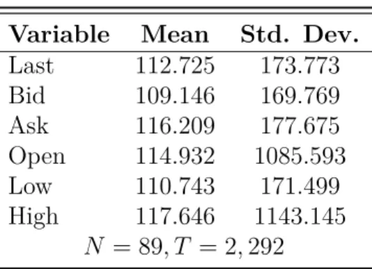
In Table 11.2, we see the mean of the Offer is above the mean of the Ask, meaning investors who are attempting to sell the CDS value it above investors who are attempting to buy them. Additionally, the Last price of the spreads (given in bps) are well varied, so that when they are used to calculate returns, there is enough variance in the data for our regression.

6.1.1 Returns and Volatility

We use the daily difference of log spreads, as in Bostanci and Yilmaz (2015), which has several benefits. Log normal returns allow us to normalize to a common unit (returns) across different pricing units, as not all credit default swaps are traded in bps. Given that the price of a CDS is normally distributed, then log(1 +ri), whereri is the daily return for

given company i, is also normally distributed.

(15)

notation introduced by Garman and Klass (1980). Letf ∈[0,1]be the fraction of the period that trading is closed, C0 be the closing price of the previous period (at time 0), O1 be the

opening price of the current period (at time f), H1 be the current period’s high during the

trading interval (between [f,1]), L1 be the current period’s low during the trading interval

(between[f,1]), and C1 be the closing price of the current period (at time 1). The variance

(square of volatility) estimator is given by:

V =V0+kVc+ (1−k)VRS (6.1)

where

k = 0.34 1.34 + n_n+1₋₁

V0 =

T n−1

n

X

i=1

(oi−¯o)2

Vc=

T n−1

n

X

i=1

(ci−¯c)2

VRS =

T n

n

X

i=1

[ui(ui−ci) +di(di+ci)]

wherek is a constant chosen such that it minimizes the variance of the estimatorV,T is the time period, n is the number of periods (in our case, n = 191, which results in k = 0.144),

o= lnO1−lnC0, c= lnC1−lnO1,u= lnH1−lnO1, d= lnL1−lnO1,o¯=

1 n

Pn

i=1oi, and

¯ c= 1

n

Pn

i=1ci. Finally, T = 12, which is the number of non-overlapping bins of size n= 191

in the sample.

6.2 News Measure

(16)

re-leases.6 _{The database contains over 119 million observations of news releases from DowJones} sources (Dow Jones Newswires, regional editions of the Wall Street Journal, Barron’s and MarketWatch) at the milisecond level, along with the corresponding International Securi-ties Identification Number (ISIN), a company identification code, for the topical company, sentiment analysis, and categorization into progressively finer topic levels. To transform this database we begin with the second coarsest level (Group) of categorization, which is composed of 51 possible different topics (not all topics appear in our sample, however). For the company-level analysis, we form a topical index for each company. Additionally, for sector-level analysis, we form a revenue weighted index for all available companies.

6.2.1 Company Level

We wish to construct an index for each company across the different news types. This index is denoted Fi,j,t, meaning the index for companyi concerning topic j at time t. In order to

construct an index for company-level events, we begin with Ii,j,l,t an indicator function for

an event, defined as

Ii,j,l,t =



  

  

1 if the lth news release about topic j for company i occured at time t

0 otherwise

(6.2)

To then aggregate these indicators to a single measure, we sum Ii,j,t across each day and

divide by the maximum sum for the time period T, as:

Fi,j,t =

PN

l=1Ii,j,l,t

max

∀t {

PN

l=1Ii,j,l,t}

(6.3)

where N is the total number of events for topic j and company i at time t. In sum, we have constructed an index between 0 and 1 which indicates how much news activity there was for a topic on each day.

(17)

6.2.2 Sector Level

We construct a basic sector-level news measure by aggregating the sum of the company-level news indicator across each sector. Let S = {S1,S2, . . . ,Sm−1,Sm−2, . . . ,Sq} be the set of

sectors, where Sm ={χ1, χ2, . . . , χM} for and M ≤ N, such that Si ∩ Sj =∅ for all i 6= j,

and where χ is the vector of companies. Thus, the basic sector level news measure Fm for

sector m is given by

Fm,j,t =

X

i∈M

Fi,j,t (6.4)

For the sector level data, we include news data of companies outside the sample of those with credit default swaps. In this model, companies without credit default swaps can still affect those that do have CDS’s. Additionally, we expect some companies to play a more vital role in representing the stability (or instability) of a sector. These adjusted sector-level mews measures, denoted _F˜_{, are the sum of the indicator measure for all companies in the} sector, each company would be given equal weight in changing the index. To represent the impact a company has on a sector, we use revenue data from Institutional Brokers’ Estimate System (I/B/E/S).7 _{We take the sum of total revenue in the sector and use a company’s} share of the revenue as their weight in the aggregation function. Thus, we have

˜

Fm,t =

P

i∈M|Ri,t|Fm,t

P

i∈M|Ri,t|

(6.5)

where Ri,t is the revenue for company i at timet.

6.3 Macroeconomic Data

(18)

Consumer Price Index for All Urban Consumers, Effective Federal Funds Rate, Quarterly Seasonally Adjusted Gross Domestic Product, Real Median Household Income in the United States, Trade Weighted U.S. Dollar Index, University of Michigan: Consumer Sentiment, and University of Michigan: Inflation Expectation. All data are from Federal Reserve Eco-nomic Data (FRED) which are observed from 2007 to 2013. There are a few important aspects to note. First, except for both of the Michigan covariates (which are monthly), the macroeconomic covariates are quarterly, while our financial data is daily (trading days). Given several years of data, there is enough variation in the macroeconomic variables to make the regression meaningful. Second, the macroeconomic variables are the value for the prior quarter, so we use these to represent economic activity for each day. Additionally, the quarterly macroeconomic covariates act as controls for the economic climate, as well as other unseen factors not included in the news measure. Third, given the high frequency of the University of Michigan covariates (Consumer Sentiment and Inflation Expectation) do represent the quite likely expected value by consumers at the time of observation. We make the simlifying assumption that the investors for which we observe financial data are the same (of the same type) as the consumer forming expectations in these surveys. In this way, these two covariates do represent investor knowledge (expectation) at the time.

7 Empirical Model

7.1 Company Level

We follow Bostanci and Yilmaz (2015) and estimate a third order vector autoregression (VAR)

yt=

3 X

h=1

Ahyt−h+εt (7.1)

(19)

and Ah’s are 89×89coefficient matrices.

7.2 Sector Level

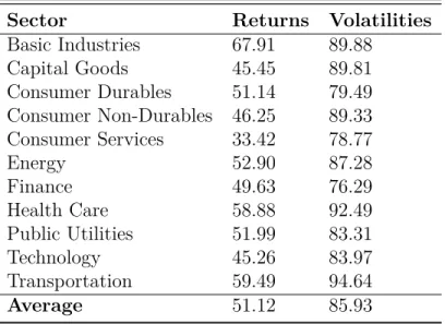
With 89 companies and a third order VAR, we would have 264 independent variables on the right-hand side. If we wished to include the company news measure F as a covariate, the regression becomes non-singular. We could impose identifying assumptions to reduce the number of covariates at the company level, but this still causes issues with non-singular matrix when estimating the coefficients. We resolve the issue of high-dimensionality by using principal component analysis (PCA) to view sector connectedness. Each credit default swap is grouped by its sector and PCA is then applied by group. For each of these PCAs, we use the first principal component when forming the new VAR, denoting the vector of first principal components as z. The use of PCA follows intuitively, as it explains the greatest source of variance in the forecast error, which the index is meant to capture. Thus, we are able to gain a strong and accurate view of connectedness, without dealing with the issues high-dimensional analysis. We will discuss the specifics of the industries in the data and results section. PCA thus allows us an easier network to interpret; instead of having to view 89 nodes and their 89×2 = 178 edge weights, we are limited to 10 to 20 nodes and their 20-40 edges, which is much more manageable. On the other hand, we lose information on connectedness of specific companies, preventing us from viewing company-level spillovers and changes in its network over time.

We again estimate a VAR(3)

zt=

3 X

h=1

Ahzt−h+ Λ ˜Ft+ ΞWt+εt (7.2)

wherezt is a11×1vector of returns or estimated volatilities for 11sectors at timet, the

Ah’s are11×11coefficient matrices, the news measure isF˜, and macroeconomic variables are

(20)

matrix andDt is adim( ˜F)×1matrix of dim( ˜F)vectors at timet, wheredim( ˜F)is the total

number of news covariates (the column size of _F˜_{). Now, each endogenous variable} _y_i_|_t_{, for}

i= 1, . . . , K, has dim( ˜F) exogenous variables, meaning the dim( ˜F) variables are specific to company i. Lastly, Ξ is a K×dim(W) coefficient matrix for the macroeconomic covariates

W.

We now discuss our identifying assumptions on the coefficient matrixΛ, imposing struc-ture so thatΛij = 0forj /∈ {dim( ˜F)·(i−1)+1,dim( ˜F)·(i−1)+2, . . . ,dim( ˜F)·(i−1)+dim( ˜F)},

where _F˜_m _{are the factors specific to sector} _m_{. However, we do not impose any structure} on the Ah’s or Ξ. In other words, factors for a company only affect that specific company

directly, but macroeconomic variables and lags of the price affect allzm,t. This is not to say

that factors for other companies do not have some effect on a particular company. Instead, these factors first affect the price (and therefore the returns or volatility) for the correspond-ing company, which then affects all other companies through its lag. In this way, there is a delayed response from investors reacting to shocks; investors spend time learning and evalu-ating the possible impacts of some shocks. Of course, the delay of the investors reaction may range widely amongst investors, so there is some importance in the unit t. A large t, such as a year, would imply a long, delayed reaction by the market in response to these shocks. As our unit is daily, we assume the market takes at least a day to react to shocks.

(21)

the Federal level to regulation at a state or even city level, depending on what connectedness we are examining.

8 Results

We begin by viewing static network plots for both company returns and price volatilities. As in Diebold and Yilmaz 2015a, we use Gephi, a program for network plots and analysis, to graph the networks8_{. For all network graphs (including those later in this paper), we} use ForceAtlas2, a node position algorithm which uses edge weights as a gravitational force. Using the company-level results as motivation for aggregation, we then transition to a dis-cussion of sector-level results. After analyzing the static sector-level networks for returns and price volatilities, we employ a rolling window to view changes in sector connectedness over time. We then view results starting at the spillover index and proceeding down to more detailed results. As it is impractical to view the thousands of networks given by our rolling window analyses, we aggregate the sector connectedness measures to net connectedness of each sector. Lastly, we conclude with a robustness check to view the sensitivity of our results to the rolling window size and H-step ahead error.

8.1 Static (Full-Sample, Unconditional) Company Level Results

Our analysis begins in Figure 11.3, which is a network of company returns. The network is symmetrically connected for all companies, as it has a circular shape, indicating equal opposing and attractive forces. There are a few noticeable exceptions, such as the strong link between two blue nodes at the bottom of the graph, which are Campbell Food and General Mills, both in the Consumer Non-Durables sector. We note that these companies are in the same sector, which follows our intuition that companies in the same sector are more highly connected. Since shocks that affect a sector are propagated throughout all companies

(22)

in the sector, the residuals are strongly correlated, and thus their edge weight is stronger. Additionally, we plot a network for company price volatility. As opposed to company returns, this network has more sparse regions along the outer edge. There still exists a strong centrality to the shape of the network, indicating equal opposing and attractive forces. Many of the companies in the same community, such as the orange in the bottom right, belong to the same sector. From the differing network shape, we infer that shocks affect volatility differently than returns or that the shocks themselves are different. In this way, price volatility is more sensitive to shocks, which follows intuition as investors are making changes throughout the trading day based on new information.

8.2 Static (Full-Sample, Unconditional) Sector Level Results

In Figure 11.5, we see the distribution of communities among each sector. We note for many of the return networks, there is a strongly dominant community. While volatility also has a dominant community, there exist smaller communities in a sector. The return network is less sensitive to shocks that affect all sectors, while price volatility network is more sensitive to shocks that affect all sectors.

We begin this section with a static network of sector returns from our PCA analysis in Figure 11.6. Now, we can distinguish interesting features of the network. For example, we observe that Technology is connected to many sectors, while not many sectors are connected to it. For example, in the center, we have a group of heavily connected sectors: Public Utilities, Consumer Non-Durables, Consumer Services, and Capital Goods. These central sectors all provide goods or services direct to households, while there are intermediary sectors between the outer edge networks. We expect the shocks to these sectors are common, such as changes in retail tax law (which would affect the aforementioned sectors), while not affecting other networks.

(23)

heavily connected as those in the center. Note the strong link between of Energy to Public Utilities and Consumer Non-Durables, which would follow as Energy is reliant on these sectors. Consumer Services, in particular, is far from many of the other sectors, indicating it is independent of shocks from all other sectors. Detecting communities as before, we note two communities, one of which contains Consumer Non-Durables, Energy, and Finance. This community has a common attribute of being fast-moving, meaning there is high quantity demanded and volatile changes are made to supply. The other community experiences a more consistent level of demand and is thus sensitive to different shocks.

8.3 Dynamic (Rolling-Sample, Conditional) Sector Level Results

Since we are motivated to aggregate the data to a sector level in order to lower the dimen-sionality, we focus solely on sector level results for dynamic analysis, for which we use a window size of 500 and an 12-step ahead error. We examine different network measures, starting from the broad view of the spillover index to the micro view ofnet connectednessby sector. In these analyses, we look at the changes before and after the addition of covariates and examine the determining factors.

(24)

then, are strongly based on the returns previous sector itself and not other sectors. For the GVD based spillover index, the estimate tends to be higher than the maximum of the Cholesky decomposition. Also, the connectedness measure is higher under GVD, as found in Klößner and Wagner (2014).

In Figure 11.9 we plot the spillover index for price volatility. Around 2008, we see a sharp increase in the spillover index, around the time of the financial crisis. We also see the advent of the big bang around mid-2010, with a return to normalcy thereafter. Exploring our various orderings and decompositions, we see the maximum and minimum for the Cholesky based index has a broad range, so price volatility is sensitive to the Cholesky ordering. We expect there exist more common factors between these sectors than with returns. The GVD based index is higher than the maximum of the Cholesky based index, save for a few exceptions.

We further collapse the data to net connectedness, as detailed in the connectedness sec-tion, to allow us to see changes to the network over time. This transformation provides a compact view of connectedness dynamics, allowing us to see the effect of the inclusion of our covariates. First, we examine the sensitivity of the net connectedness measure to the Cholesky ordering. For further analyses, we focus on the average net connectedness across 10,000 random permutations. While we lose information on the connectedness between sec-tors, we still can glean the spillover of one sector towards all others and all others to that sector.

(25)

maximum and minimum values for the net connectedness measures have similar features to Figure 11.10.

In 11.11, we better observe the overall changes in sector returnnet connectedness. Around 2008, there is a sharp decrease in net connectedness in finance, for example, which aligns with the financial crisis. Conversely, we see increases in net connectedness within Energy, Health Care, and Public Utilities. So, shocks to Finance, Energy, Health Care, and Public Utilities explained the returns for one another more strongly during this period. We see a notable changes around 2010, which we attribute to the big bang, which is followed by a return to normalcy.

We can see the effect of including covariates in Figure 11.12. Overall, many of the abrupt changes in net connectedness are lessened when covariates are added. For example, the sharp decrease for Finance in 2008 is lessened. However, long-run trends, such as the slower decrease in Technology around 2010, are increased. In other words, knowledge of these events lessens the impact to net connectedness for sudden changes, but increases the impact of changes over a longer run. If the long-run trend is due to the big bang, including covariates would strengthen it due to a stronger correlation among the errors, as the big bang underlies all sectors.

For sector price volatility, we observe sector net connectedness before the inclusion of covariates in Figure 11.13. For many sectors, such as Basic Industries, thenet connectedness measure is around 0, indicating equal to connectedness and from connectedness. There are notable exceptions, such as Energy, with experiences sharp dips and increases. We expect, then, that energy shares covariates with other sectors the most out of the other sector covariates. With our identifying assumptions, we are restricted to these shared covariates being macroeconomic factors, as sector-specific factors cannot be shared (i.e. Energy analyst ratings cannot affect Consumer Durables volatility, by our assumption).

(26)

in the average around 2008 for Energy is lower than the average for sector volatility net connectedness without covariates. Including investor knowledge and macroeconomic climate causes errors to be more highly correlated and thus spillovers increase. If net connectedness is becoming more volatile, that means that from connectedness and to connectedness are also volatile. As from connectedness sums to unity, the spillovers must be transferring to other sectors or from other sectors for a specific sector if there is a change in net connect-edness. In conclusion, including covariates for price volatility increases the volatility of net connectedness for each sector.

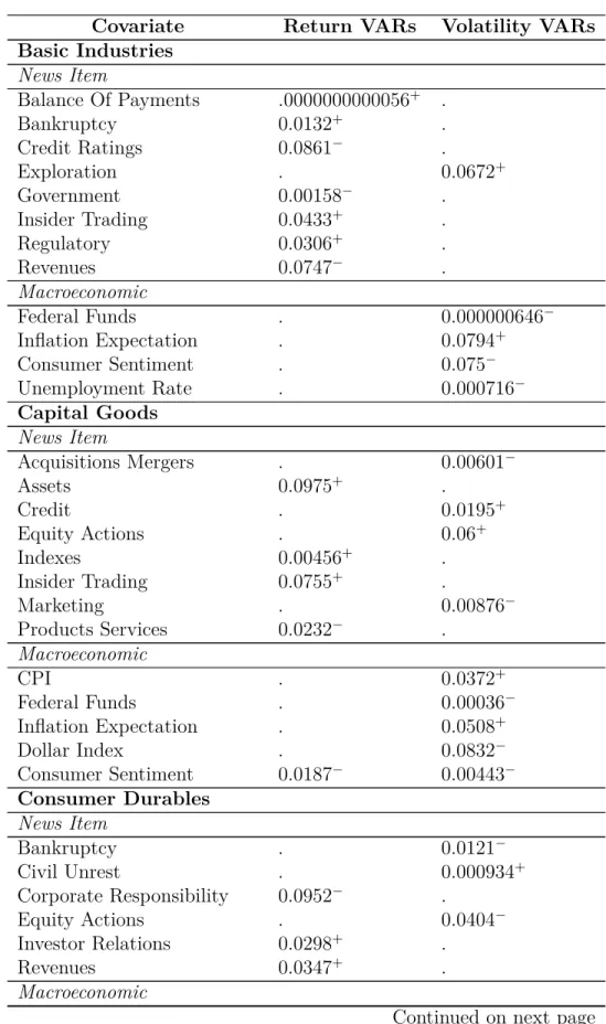
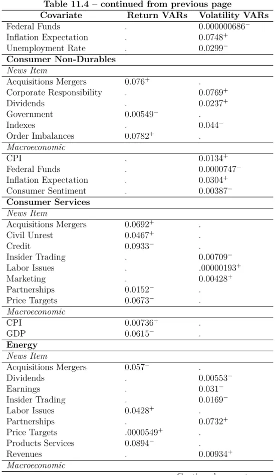
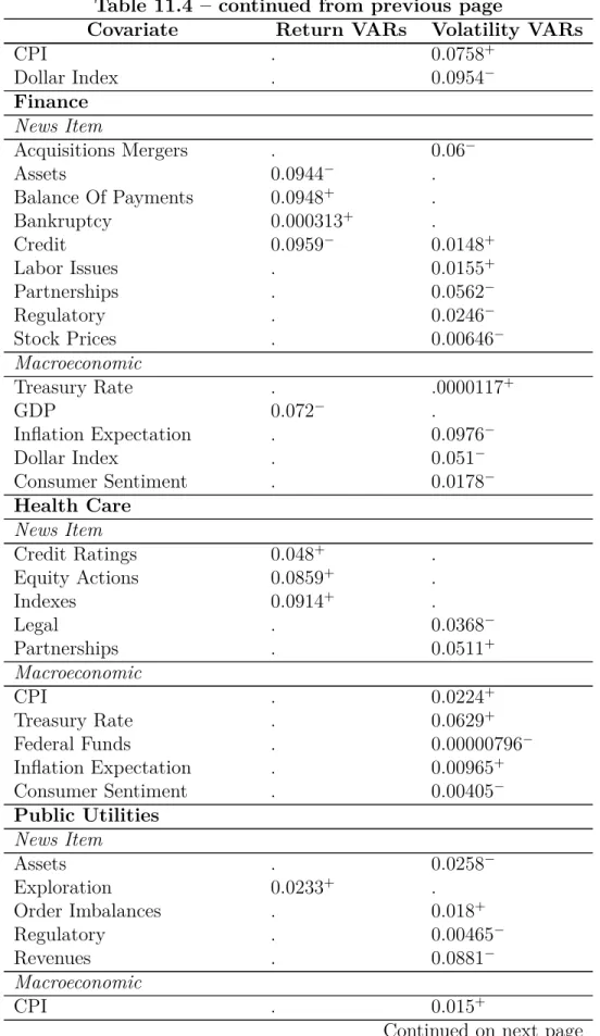
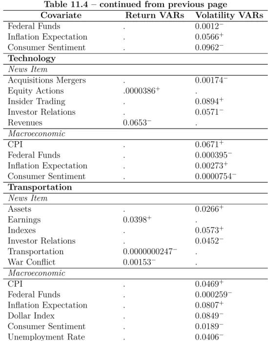
We transition to discussion of significant covariates in Table 11.4. For the return VARs, we see that news items compose most of the significant covariates, whereas macroeconomic covariates are not significant. We see that sectors that had strong connections share common covariates, such as news about Insider Trading among Basic Industries, Capital Goods, Consumer Services, and Energy. As these coefficients were originally in the residuals, and are of the same sign, we have reduced the residual and thus changed the underlying connectedness estimation. Additionally, we observe there are factors unique to some sectors, such as Price Targets news for Consumer Services or War Conflict news for Transportation As these factors were not common in all the residuals, the underlying connectedness measure changes in a different way. Overall, we see many different factors are significant and thus have changed the residuals and reduced the sum of squared residuals.

(27)

dynamics drive volatilities and returns.

9 Robustness

We sample spillover indices andnet connectednessfor select sectors to examine the effects of changing the window size andH-step ahead error. Changes in the window size indicates the strength of past factors on the current connectedness measure. For example, a large window size indicates factors (such as returns) further in the past affect returns in the future. We also examine changes in theH-step ahead error. We examined the robustness of each sector and select the sector which is affected most these changes. For net connectedness of returns without covariates, we examine the robustness of Basic Industries. Additionally, for net connectedness of price volatility with covariates, we examine the robustness of Energy.

In Figure 11.15, as window size increases, we lose finer details on changes in connected-ness: a larger window means means larger samples, making a rolling window (by adding and dropping one observation at time) have less changes in the regression overall. This is not necessarily a detriment, as we expect there to be some appropriate window size which rep-resents the extent of investors consideration to the past. Additionally, for changes inH-step ahead error, we see there do not exist detectable changes to the spillover index. Our baseline index is 12-step ahead, 500 day window size, which we compare among the other sizes. We see that despite changes in the H-step and window size, the our choice still captures the overall trends present in all facets, save for some minor fluctuations

(28)

measure is robust. For our default window size and H-step, we see, comparatively, there is a different in the rise of net connectedness around 2011, with our baseline being a minor increase. Still, we find the overall trend follows throughout each facet.

Lastly, we select Energy price volatility with covariates in Figure 11.17. We see as window size increases, magnitude decreases, as expected. Additionally, asH-step ahead error increases, the magnitude increases. Even with the smallest magnitude across our window size is 200 and 6-step errors at, we still see a notable drop in net connectednessaround 2008. Thus the trends we detect throughout our analyses are apparent despite changes in window size andH-step ahead error. Our choices find an appropriate middle ground that still covers sudden changes, such as the dramatic decrease around 2008, with the value not being as extreme as for a window size of 150 and 12-step ahead.

10 Conclusion

We use the Diebold-Yilmaz connectedness measure to study the spillovers between 89 com-pany credit default swaps over the period of 2007 to 2013. In order to make interpretation more manageable, we use Principal Component Analysis to reduce the dimensionality of company prices to a sector-level. We include news and macroeconomic covariates in the un-derlying VAR for returns and examine the changes innet connectednessbefore and after the inclusion of our covariates. This is in contrast to previous agnostic views taken when using the Diebold-Yilmaz connectedness measure, which look to examine what events took place during changes in connectedness, but do not have a way to test the underlying statistical significance of the events nor deal with a large number of events.

(29)

(30)

11 Appendix

11.1 Tables

Table 11.1: Connectedness Table

x1 x2 · · · xN From Others

x1 dH11 dH12 · · · dH1N

PN

j=1d

H

1j, j 6= 1

x2 dH11 dH12 · · · dH1N

PN

j=1d

H

1j, j 6= 2

... ... dH₁₂ ... ... ...

xN dHN1 dHN2 · · · dHN N

PN

j=1d

H

1j, j 6=N

To Others PN

i=1d

H i1, i6= 1

PN

i=1d

H

i2, i6= 2 · · ·

PN

i=1d

H

iN, i6=N N1

PN

i=1d

H ij, i6=j

(31)

Table 11.2: Summary Statistics

Variable Mean Std. Dev.

Last 112.725 173.773

Bid 109.146 169.769

Ask 116.209 177.675

Open 114.932 1085.593

Low 110.743 171.499

High 117.646 1143.145

N = 89, T = 2,292

(32)

Table 11.3: Principal Component Variance Share

Sector Returns Volatilities

Basic Industries 67.91 89.88

Capital Goods 45.45 89.81

Consumer Durables 51.14 79.49

Consumer Non-Durables 46.25 89.33

Consumer Services 33.42 78.77

Energy 52.90 87.28

Finance 49.63 76.29

Health Care 58.88 92.49

Public Utilities 51.99 83.31

Technology 45.26 83.97

Transportation 59.49 94.64

Average 51.12 85.93

(33)

Table 11.4: p-values and Coefficient Sign for Static VARs

Covariate Return VARs Volatility VARs Basic Industries

News Item

Balance Of Payments .0000000000056+ _.

Bankruptcy 0.0132+ _.

Credit Ratings 0.0861− _.

Exploration . 0.0672+

Government 0.00158− _.

Insider Trading 0.0433+ .

Regulatory 0.0306+ _.

Revenues 0.0747− _.

Macroeconomic

Federal Funds . 0.000000646−

Inflation Expectation . 0.0794+

Consumer Sentiment . 0.075−

Unemployment Rate . 0.000716−

Capital Goods

News Item

Acquisitions Mergers . 0.00601−

Assets 0.0975+ _.

Credit . 0.0195+

Equity Actions . 0.06+

Indexes 0.00456+ _.

Insider Trading 0.0755+ .

Marketing . 0.00876−

Products Services 0.0232− _.

Macroeconomic

CPI . 0.0372+

Dollar Index . 0.0832−

Consumer Sentiment 0.0187− 0.00443−

Consumer Durables

News Item

Bankruptcy . 0.0121−

Civil Unrest . 0.000934+

Corporate Responsibility 0.0952− _.

Equity Actions . 0.0404−

Investor Relations 0.0298+ .

Revenues 0.0347+ _.

Macroeconomic

(34)

Table 11.4 – continued from previous page

Covariate Return VARs Volatility VARs

Consumer Non-Durables

News Item

Acquisitions Mergers 0.076+ _.

Corporate Responsibility . 0.0769+

Dividends . 0.0237+

Government 0.00549− _.

Indexes . 0.044−

Order Imbalances 0.0782+ _.

Macroeconomic

CPI . 0.0134+

Consumer Services

News Item

Acquisitions Mergers 0.0692+ .

Civil Unrest 0.0467+ _.

Credit 0.0933− _.

Insider Trading . 0.00709−

Labor Issues . .00000193+

Marketing . 0.00428+

Partnerships 0.0152− _.

Price Targets 0.0673− _.

Macroeconomic

CPI 0.00736+ _.

GDP 0.0615− _.

Energy

News Item

Acquisitions Mergers 0.057− _.

Dividends . 0.00553−

Earnings . 0.031−

Insider Trading . 0.0169−

Labor Issues 0.0428+ _.

Partnerships . 0.0732+

Price Targets .0000549+ _.

Products Services 0.0894− _.

Revenues . 0.00934+

Macroeconomic

(35)

CPI . 0.0758+

Finance

News Item

Assets 0.0944− _.

Balance Of Payments 0.0948+ .

Bankruptcy 0.000313+ _.

Credit 0.0959− 0.0148+

Labor Issues . 0.0155+

Partnerships . 0.0562−

Regulatory . 0.0246−

Stock Prices . 0.00646−

Macroeconomic

Treasury Rate . .0000117+

GDP 0.072− _.

Inflation Expectation . 0.0976−

Health Care

News Item

Credit Ratings 0.048+ .

Equity Actions 0.0859+ _.

Indexes 0.0914+ _.

Legal . 0.0368−

Partnerships . 0.0511+

Macroeconomic

CPI . 0.0224+

Treasury Rate . 0.0629+

Public Utilities

News Item

Assets . 0.0258−

Exploration 0.0233+ _.

Order Imbalances . 0.018+

Regulatory . 0.00465−

Revenues . 0.0881−

Macroeconomic

CPI . 0.015+

(36)

Technology

News Item

Equity Actions .0000386+ .

Insider Trading . 0.0894+

Investor Relations . 0.0571−

Revenues 0.0653− _.

Macroeconomic

CPI . 0.0671+

Transportation

News Item

Assets . 0.0266+

Earnings 0.0398+ .

Indexes . 0.0573+

Investor Relations . 0.0452−

Transportation 0.0000000247− _.

War Conflict 0.00153− _.

Macroeconomic

CPI . 0.0469+

p-values for covariates in each VAR that were of 10% significance or better. All values are given to three significant digits. A “.” indicates the value was not significant in the estimated VAR. A minus sign (−_{) indicates the sign of the coefficient in the VAR is negative, while a plus sign (}+)

(37)

11.2 Figures

Figure 11.1: CDO Structural Diagram

(38)

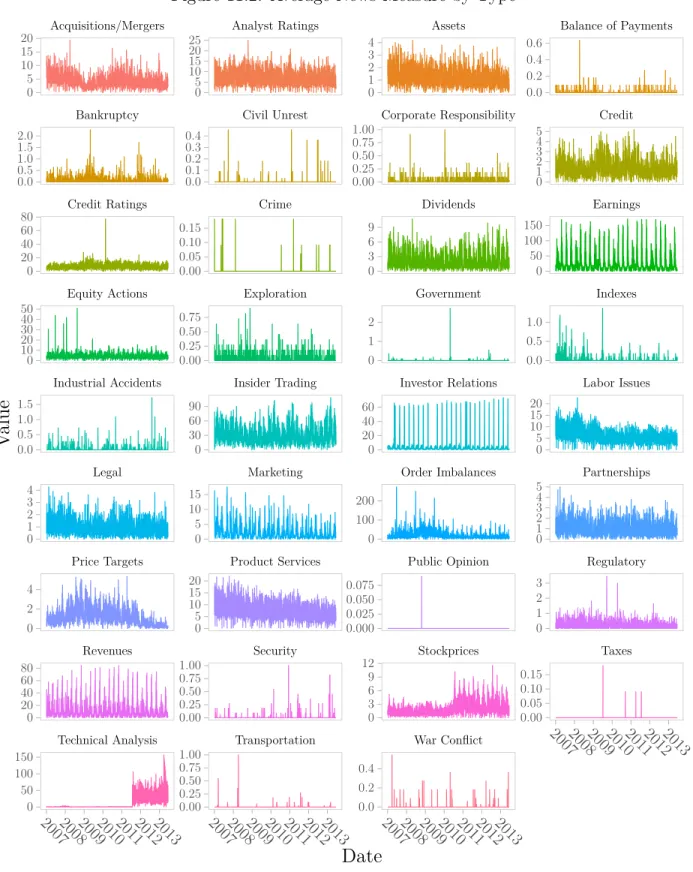
Figure 11.2: Average News Measure by Type

Technical Analysis Transportation War Conflict

Revenues Security Stockprices Taxes Price Targets Product Services Public Opinion Regulatory

Legal Marketing Order Imbalances Partnerships Industrial Accidents Insider Trading Investor Relations Labor Issues

Equity Actions Exploration Government Indexes Credit Ratings Crime Dividends Earnings

Bankruptcy Civil Unrest Corporate Responsibility Credit Acquisitions/Mergers Analyst Ratings Assets Balance of Payments

2007200820092010201120122013 2007200820092010201120122013 2007200820092010201120122013

2007200820092010201120122013 0.0 0.2 0.4 0.6 0 1 2 3 4 5 0 50 100 150 0.0 0.5 1.0 0 5 10 15 20 0 1 2 3 4 5 0 1 2 3 0.00 0.05 0.10 0.15 0 1 2 3 4 0.00 0.25 0.50 0.75 1.00 0 3 6 9 0 1 2 0 20 40 60 0 100 200 0.000 0.025 0.050 0.075 0 3 6 9 12 0.0 0.2 0.4 0 5 10 15 20 25 0.0 0.1 0.2 0.3 0.4 0.00 0.05 0.10 0.15 0.00 0.25 0.50 0.75 0 30 60 90 0 5 10 15 0 5 10 15 20 0.00 0.25 0.50 0.75 1.00 0.00 0.25 0.50 0.75 1.00 0 5 10 15 20 0.0 0.5 1.0 1.5 2.0 0 20 40 60 80 0 10 20 30 40 50 0.0 0.5 1.0 1.5 0 1 2 3 4 0 2 4 0 20 40 60 80 0 50 100 150

Date

Value

(39)

Figure 11.3: Static Company Return Network Graph

(40)

Figure 11.4: Static Company Price Volatility Network Graph

(41)

Figure 11.5: Distribution of Companies Among Modularities

Technology Transportation

Finance Health Care Public Utilities

Consumer Non-Durables Consumer Services Energy

Basic Industries Capital Goods Consumer Durables

Return Volatility Return Volatility

Return Volatility 0 1 2 3 4 5 0 2 4 6 0 1 2 3 4 0 2 4 6 8 0 5 10 0 1 2 3 4 0 1 2 3 0 1 2 3 4 5 0 2 4 6 0.0 2.5 5.0 7.5 0 2 4 6

Network

Frequency

Group

0 1 2 3

(42)

Figure 11.6: Static Sector Network Graph

Basic Industries Capital Goods

Consumer Durables Consumer Non-Durables

Consumer Services Energy

Finance Health Care

Public Utilities

Technology

Transportation

(43)

Figure 11.7: Static Sector Network Graph

Basic Industries

Capital Goods Consumer Durables

Consumer Non-Durables

Consumer Services

Energy

Finance

Health Care

Public Utilities

(44)

Figure 11.8: Spillover Index for Returns without Covariates

0 25 50 75 100

2007 2008 2009 2010 2011 2012 2013

Date

Index

(45)

Figure 11.9: Spillover Index for Volatilities without Covariates

0 25 50 75 100

2007 2008 2009 2010 2011 2012 2013

Date

Index

Diebold-Yilmaz spillover index for volatilities without sector-specific and macroeconomic covariates. Average value and maximum and minimum spillover index across all VAR orderings for Cholesky decomposition are given by the black line and gray ribbon, respectively. 25% and 75% bounds for the Cholesky Decomposition across 10,000 random permutations are given by the red ribbon. Index for generalized variance decomposition (GVD) is given by the blue line.

(52)

Figure 11.16: Net Basic Industries Return Connectedness with Covariates

2007 2008 2009 2010 2011 2012 2013 2007 2008 2009 2010 2011 2012 2013 2007 2008 2009 2010 2011 2012 2013 -10

0 10 20

-10 0 10 20

Date

Value

(53)

Figure 11.17: Net Energy Volatility Connectedness without Covariates

2007 2008 2009 2010 2011 2012 2013 2007 2008 2009 2010 2011 2012 2013 2007 2008 2009 2010 2011 2012 2013 -300

-200 -1000

-300 -200 -1000

Date

Value

(54)

Bibliography

Baruník, Jozef, Evžen Kočenda, and Lukáš Vácha. 2016. “Asymmetric connectedness on the US stock market: Bad and good volatility spillovers”. Journal of Financial Markets 27:55–78.

Bastian, Mathieu, Sebastien Heymann, and Mathieu Jacomy. 2009. Gephi: An Open Source Software for Exploring and Manipulating Networks.http://www.aaai.org/ocs/index.

php/ICWSM/09/paper/view/154.

Blondel, Vincent D, et al. 2008. “Fast unfolding of communities in large networks”. Journal of statistical mechanics: theory and experiment 2008 (10): P10008.

Bostanci, Gorkem, and Kamil Yilmaz. 2015. “How Connected is the Global Sovereign Credit Risk Network?” Available at SSRN 2647251.

Crouhy, Michel G, Robert A Jarrow, and Stuart M Turnbull. 2008. “The subprime credit crisis of 2007”. The Journal of Derivatives 16 (1): 81–110.

Demirer, Mert, et al. 2015. “Estimating global bank network connectedness”.

Diebold, Francis X, and Kamil Yilmaz. 2012. “Better to give than to receive: Predictive directional measurement of volatility spillovers”. International Journal of Forecasting 28 (1): 57–66.

Diebold, Francis X, and Kamil Yilmaz. 2015a.Financial and Macroeconomic Connectedness: A Network Approach to Measurement and Monitoring. Oxford University Press, USA.

— . 2009. “Measuring financial asset return and volatility spillovers, with application to global equity markets”. The Economic Journal 119 (534): 158–171.

(55)

Diebold, Francis X, and Kamil Yılmaz. 2014. “On the network topology of variance decom-positions: Measuring the connectedness of financial firms”.Journal of Econometrics 182 (1): 119–134.

Diebold, Francis X, and Kamil Yilmaz. 2015b. “Trans-atlantic equity volatility connected-ness: Us and european financial institutions, 2004–2014”. Journal of Financial Econo-metrics 14 (1): 81–127.

Diebold, Francis X, Kamil Yilmaz, et al. 2011. “Equity market spillovers in the Americas”. Financial stability, monetary policy, and central banking 15:199–214.

Duffie, Darrell, Leandro Saita, and Ke Wang. 2007. “Multi-period corporate default predic-tion with stochastic covariates”. Journal of Financial Economics 83 (3): 635–665.

Fonseca, Jose De, and Katrin Gottschalk. 2012. The co-movement of credit default swap spreads, stock market returns and volatilities: evidence from Asia-Pacific markets. Tech. rep. working paper.

Gibson, Michael S. 2004. “Understanding the risk of synthetic CDOs”.

Hamilton, James Douglas. 1994. Time series analysis. Vol. 2. Princeton university press Princeton.

Jacomy, Mathieu, et al. 2014. “ForceAtlas2, a continuous graph layout algorithm for handy network visualization designed for the Gephi software”. PloS one 9 (6): e98679.

Klößner, Stefan, and Rodrigo Sekkel. 2014. “International spillovers of policy uncertainty”. Economics Letters 124 (3): 508–512.

Klößner, Stefan, and Sven Wagner. 2014. “Exploring all VAR orderings for calculating spillovers? yes, we can!—a note on Diebold and Yilmaz (2009)”.Journal of Applied Econo-metrics 29 (1): 172–179.

(56)

Li, David X. 2000. “On default correlation: A copula function approach”. The Journal of Fixed Income 9 (4): 43–54.

Longstaff, Francis A, and Arvind Rajan. 2008. “An empirical analysis of the pricing of collateralized debt obligations”. The Journal of Finance 63 (2): 529–563.

Longstaff, Francis A, et al. 2011. “How sovereign is sovereign credit risk?” American Eco-nomic Journal: MacroecoEco-nomics 3 (2): 75–103.

Lütkepohl, Helmut. 2005.New introduction to multiple time series analysis. Springer Science & Business Media.

Maghyereh, Aktham I, Basel Awartani, and Elie Bouri. 2016. “The directional volatility connectedness between crude oil and equity markets: New evidence from implied volatility indexes”. Energy Economics 57:78–93.

Markowitz, Harry. 1952. “Portfolio selection”.The journal of finance 7 (1): 77–91.

Pan, Jun, and Kenneth J Singleton. 2008. “Default and recovery implicit in the term structure of sovereign CDS spreads”. The Journal of Finance 63 (5): 2345–2384.

Pericoli, Marcello, and Marco Taboga. 2015. “Decomposing euro area sovereign spreads: credit, liquidity and convenience”.

Pesaran, M Hashem, and Yongcheol Shin. 1998. “An autoregressive distributed-lag modelling approach to cointegration analysis”. Econometric Society Monographs 31:371–413.

Wang, Gang-Jin, et al. 2016. “Who are the net senders and recipients of volatility spillovers in China’s financial markets?” Finance research letters 18:255–262.

Yang, Dennis, and Qiang Zhang. 2000. “Drift-independent volatility estimation based on high, low, open, and close prices”.The Journal of Business 73 (3): 477–492.