THE RELATIONSHIP BETWEEN MOLECULAR GAS, H
I, AND STAR FORMATION IN THE LOW-MASS,
LOW-METALLICITY MAGELLANIC CLOUDS
Katherine E. Jameson1, Alberto D. Bolatto1, Adam K. Leroy2, Margaret Meixner3, Julia Roman-Duval3,
Karl Gordon3, Annie Hughes4, Frank P. Israel5, Monica Rubio6, Remy Indebetouw7,8, Suzanne C. Madden9, Caroline Bot10, Sacha Hony11, Diane Cormier11, Eric W. Pellegrini12, Maud Galametz13, and George Sonneborn14
1
Astronomy Department and Laboratory for Millimeter-wave Astronomy, University of Maryland, College Park, MD 20742, USA;kjameson@astro.umd.edu
2
Department of Astronomy, The Ohio State University, 4051 McPherson Laboratory, 140 West 18th Avenue, Columbus, OH 43210, USA
3Space Telescope Science Institute, 3700 San Martin Dr., Baltimore, MD 21218, USA 4
Max-Planck-Institut für Astronomie, Königstuhl 17 D-69117 Heidelberg, Germany
5
Sterrewacht Leiden, Leiden University, P.O. Box 9513, 2300 RA Leiden, The Netherlands
6
Departamento de Astronoma, Universidad de Chile, Casilla 36-D, Chile
7
Department of Astronomy, University of Virginia, P.O. Box 400325, Charlottesville, VA 22904, USA
8
National Radio Astronomy Observatory, 520 Edgemont Road, Charlottesville, VA 22903, USA
9
Laboratoire AIM, CEA, Université Paris VII, IRFU/Service d’Astrophysique, Bat. 709, F-91191 Gif-sur-Yvette, France
10Observatoire Astronomique de Strasbourg, Université de Strasbourg, CNRS, UMR 7550, 11 rue de l’Université, F-67000 Strasbourg, France 11
Institut für Theoretische Astrophysik, Zentrum für Astronomie, Universität Heidelberg, Albert-Ueberle-Str. 2, D-69120 Heidelberg, Germany
12
Department of Physics and Astronomy, University of Toledo, 2801 West Bancroft Street, Toledo, OH 43606, USA
13
European Southern Observatory, Karl-Schwarzschild-Str. 2, D-85748 Garching-bei-München, Germany
14NASA Goddard Space Flight Center, Observational Cosmology Laboratory, Code 665, Greenbelt, MD 20771, USA Received 2015 October 23; revised 2016 April 11; accepted 2016 April 25; published 2016 June 27
ABSTRACT
The Magellanic Clouds provide the only laboratory to study the effects of metallicity and galaxy mass on molecular gas and star formation at high(∼20 pc)resolution. We use the dust emission from HERITAGEHerschel
data to map the molecular gas in the Magellanic Clouds, avoiding the known biases of CO emission as a tracer of
H2. Using our dust-based molecular gas estimates, wefind molecular gas depletion times(tdepmol)of∼0.4 Gyr in the Large Magellanic Cloud and∼0.6 in the Small Magellanic Cloud at 1 kpc scales. These depletion times fall within the range found for normal disk galaxies, but are shorter than the average value, which could be due to recent bursts in star formation. Wefind no evidence for a strong intrinsic dependence of the molecular gas depletion time on metallicity. We study the relationship between the gas and the star formation rate across a range of size scales from 20 pc to 1 kpc, including how the scatter intdepmol changes with the size scale, and discuss the physical
mechanisms driving the relationships. We compare the metallicity-dependent star formation models of Ostriker et al. and Krumholz to our observations andfind that they both predict the trend in the data, suggesting that the inclusion of a diffuse neutral medium is important at lower metallicity.
Key words:galaxies: dwarf– galaxies: evolution– ISM: clouds–Magellanic Clouds
Supporting material:data behindfigures
1. INTRODUCTION
Star formation plays a critical role in shaping how galaxies form and evolve. Understanding the molecular gas content of low-mass, low-metallicity galaxies and its relationship to the star formation rate is necessary to understand how the gas mass fractions evolve with redshift(e.g., Tacconi et al.2010; Genzel et al.2012)and how the star formation efficiency depends on galaxy mass and metallicity (e.g., Bolatto et al. 2011; Krumholz et al. 2011; Saintonge et al.2011). Both are critical for understanding the“galaxy mass function”and drivers of the star formation history of the universe.
Our current knowledge of the extragalactic relationship between gas and star formation comes from studies of mostly high-metallicity, high-mass nearby galaxies that use 12CO to trace the molecular gas. The original work to quantitatively compare the star formation rate to the gas density by Schmidt (1959)found a power-law relationship, generally referred to as the “star formation law.” More recent studies of the extragalactic star formation law follow the work of Kennicutt (1989, 1998), which used primarily disk-averaged measure-ments of the surface density of total gas (Sgas= S + SH2 HI)
and star formation rate(SSFR). They found that the relationship
between Sgas and SSFR follows a power-law distribution
(S µ S+p SFR gas
1 ). Studies at higher resolution found that the
general power-law trend continued, but only within the molecular-dominated regimes and thatSmol and SSFR follow
an approximately linear power-law relation(Bigiel et al.2008, 2011; Schruba et al.2011; Rahman et al.2012). At lower gas surface densities, where HI dominates the total gas budget, they see a steep fall-off in the relationship. Resolved galaxy studies show that while the total gas continues to be correlated with the star formation rate within galaxies, the molecular gas correlates best with the star formation rate.
Due to the nearly linear power-law slope of the relationship between Smol and SSFR, a convenient way to quantify the
relationship is the molecular gas depletion time: tdepmol= Smol SSFR. The depletion time can be thought of as
properties and environment (Leroy et al. 2013b)suggest that star formation is a local process based on the conditions within giant molecular clouds (GMCs).
The conclusions from studies of mostly mass, high-metallicity disk galaxies may not extend to lower high-metallicity star-forming dwarf galaxies where the interstellar medium (ISM)is dominated by atomic gas. The lack of metals produce different physical conditions that potentially affect the molecular gas fraction and how star formation proceeds within the galaxy. For example, the galaxies will have lower dust-to-gas ratios, which results in lower extinctions and higher photodissociation rates. The Large and Small Magellanic Clouds (LMC, SMC) provide ideal laboratories to study the physics of star formation at low mass, M*,LMC=2´109 M☉
and M*,SMC=3´108 M☉ (Skibba et al. 2012), and low
metallicity, ZLMC~1 2Z☉ (Russell & Dopita 1992) and
☉
~
ZSMC 1 5Z (Dufour1984; Kurt et al.1999; Pagel 2003), due to their proximity and our ability to achieve high spatial resolution (∼10 pc).
Tracing the molecular gas at low metallicity is difficult because CO, the most common tracer ofH2, emits weakly and is often undetected. The Magellanic Clouds have been studied extensively in12CO with the earliest surveys completed using the Columbia 1.2 m telescope (Cohen et al. 1988; Rubio et al. 1991). The early survey of both Clouds completed by Israel et al. (1993) using the Swedish-ESO Submillimetre Telescope showed the CO emission to be under-luminous compared to the Milky Way by a factor of∼3 in the LMC and ∼10 in the SMC. Since then, many large-scale surveys have been completed for the LMC (Fukui et al. 2008; Wong et al.2011)and SMC(Rubio et al.1993; Mizuno et al.2001; Muller et al. 2010).H2 gas is expected to be more prevalent than CO at low metallicity due to the increased ability ofH2to self-shield against dissociating UV photons compared to CO. Both observations and modeling suggest that ∼30%–50% of the H2in the solar neighborhood resides in a“CO-faint”phase
(e.g., Grenier et al. 2005; Wolfire et al. 2010; Planck Collaboration et al.2011), similar to the estimated fraction of H2 in the LMC(e.g., Roman-Duval et al. 2010; Leroy et al.
2011). Studies of the SMC have found that this phase encompasses 80%–90% of all the H2 (Israel 1997; Pak et al.
1998; Leroy et al. 2007, 2011; Bolatto et al. 2011), likely dominating the molecular reservoir available for star formation. Using dust emission to estimate the molecular gas in low-metallicity systems avoids the biases of CO and can trace“ CO-faint”molecular gas. This method of tracing the molecular gas using dust emission in the Magellanic Clouds wasfirst applied by Israel (1997) using IRAS data, and later by Leroy et al. (2007,2009)in the SMC and Bernard et al.(2008)in the LMC using Spitzer data. Bolatto et al. (2011) further refined the methodology and created a map of H2 in the SMC using dust continuum emission from Spitzer and studied the spatial correlation between the atomic gas, molecular gas, and star formation rate. When using the dust-based molecular gas estimate, they found thattdepmolis consistent with the values seen in more massive disk galaxies. Combining the dust-based molecular gas estimate with the atomic gas traced by HI showed that the analytic star formation models of Krumholz et al. (2009) and Ostriker et al. (2010) predicted the trend in the data.
In this work we produce an estimate of the molecular gas using dust emission traced byHerschelin the LMC and SMC.
While the SMC is lower metallicity, the geometry is poorly constrained and it shows clear signs of disturbance from interaction with the LMC and the Milky Way, which makes it problematic for comparisons against models created for galactic disks. We adopt a higher inclination angle for the SMC than was used in Bolatto et al.(2011)to explore how that affects the results. The LMC is nearly face-on with a well-constrained inclination angle and has a clear disk morphology, which minimizes the uncertainty in the analysis.
We compare the new dust-based molecular gas estimates and atomic gas to the star formation rate in both galaxies and to the existing studies of large disk galaxies. In Sections2and 3we outline the observations and how we convert them to physical quantities. Section 4 presents the main results of this study, focusing on the relationship between molecular gas and star formation, and the effect of scale. We discuss the implications of the results and compare the observations to star formation model predictions in Section 5. Finally, we summarize the conclusions from this study of the LMC and SMC in Section6.
2. OBSERVATIONS
2.1.Herschel Data
The far-IR images come from theHerschelInventory of the Agents of Galaxy Evolution in the Magellanic Clouds key project (HERITAGE; Meixner et al. 2013). HERITAGE mapped both the LMC and SMC at 100, 160, 250, 350, and 500μm with the Spectral and Photometric Imaging Receiver (SPIRE), and the Photodetector Array Camera and Spectro-meter (PACS) instruments. Information on the details of the data calibration, reduction, and uncertainty can be found in Meixner et al.(2013).
For this work, we apply further background subtraction. First, we remove the foreground Milky Way cirrus emission. Following Gordon et al.(2014) (based on Bot et al.2004), we estimate the foreground cirrus emission by using the relation-ship between IR dust emission and HIfrom Desert et al.(1990) and scaling the integrated HIintensity map over the velocities of the Milky Way emission in the direction of the LMC by applying the conversion factors 1.073, 1.848, 1.202, and 0.620 (MJy sr−1/102− cm−2) for 100μm, 160μm, 250μm, and 350μm images, respectively. The median estimated cirrus emission was 5.7, 9.9, 6.4, and 3.3 MJy sr−1for the 100, 160, 250, and 350μm images.
Second, we set the images to comparable zero-points: the outskirts of the PACS images were set to the COBE and IRAS data emission levels while the outskirts of the SPIRE images were set to zero due to the lack of similar large-scale coverage at the longer wavelengths. After subtracting the cirrus emission, we chose six regions in the outskirts of the LMC with no emission in theHerschel or HI images,fit a plane to the median values of the regions, and subtract the plane. The cirrus subtraction and background subtraction had primarily minor effects on the images, with thefinal image values being lower by 7%, 9%, 2%, and 2% on average for the 100, 160, 250, and 350μm images in regions with a signal-to-noise ratio (S/N)>3.
2.2. HIData
(1999), both combine Australian Telescope Compact Array (ATCA)and Parkes 64 m radio telescope data. The interfero-metric ATCA data set the map resolution at 1′(r∼20 pc in the SMC andr∼15 pc in the LMC), but the data are sensitive to all size scales due to the combination of interferometric and single-dish data.
The observed brightness temperature of the 21 cm line emission is converted to HI column density (NHI) assuming
optically thin emission using
( )
ò
= ´ -
-N 1.823 10 cm T v dv
K km s B .
H 18
2
1 I
Wefind rms column densities of 8.0×1019cm−2in the LMC map and 5.0 × 1019cm−2 in the SMC map. We convert column density to surface mass density(SHI)using
☉
S = ´ -
-⎛ ⎝
⎜ ⎞
⎠ ⎟
i M N
1.4 cos 8.0 10 pc
cm ,
H 21
1
2 H
I I
where the factor of 1.4 accounts for He andiis the inclination angle.
While the assumption of optically thin HIemission is likely appropriate throughout much of the galaxies, there are regions with optically thick emission, which would cause NHI to be
underestimated. While a statistical correction for HI optical depth in the SMC exists(Stanimirovićet al.1999), none exists for the LMC. Additionally, nearby surveys of HI (i.e., THINGS; Walter et al. 2008) make no optical depth corrections. We chose not to make any optical depth corrections to the HI maps as the statistical corrections in the SMC are generally small(increases the total HImass by 10%; Stanimirović et al. 1999) and an accurate optical depth correction would require assuming a spin temperature.
2.3. CO Data
We use integrated12CO(1–0)intensity maps from the 4 m NANTEN radio telescope (half power beam width of 2 6 at 115 GHz)for the LMC(Fukui et al.2008)and SMC(Mizuno et al.2001). The LMC and SMC velocity integrated maps have typical 3σ noise of ∼1.2 K km s−1 and ∼0.45 K km s−1, respectively. For the LMC, there is also the higher resolution and sensitivity Magellanic Mopra Assessment (MAGMA) Survey, which used the 22 m Mopra telescope of the Australia Telescope National Facility to follow-up the NANTEN survey with 40″angular resolution and 1σsensitivity of 0.2 K km s−1 (Wong et al. 2011). However, the MAGMA survey is not complete as they only mapped regions with detected CO in the NANTEN map. Because the CO maps are only used to identify molecular regions and do not affect the final resolution of our molecular gas maps, we use the higher coverage NANTEN maps in our molecular gas mapping process and then, in the LMC, we compare thefinal dust-based molecular gas maps to the higher resolution MAGMA data.
2.4. Hαand Spitzer 24μm Data
We combine images ofHaand 24μm dust emission to trace recent star formation. For the LMC we use the calibrated, continuum-subtracted Hα map from the Southern Hα Sky Survey Atlas(Gaustad et al.2001)at 0 8 resolution. We correct theHamaps for the line-of-sight Milky Way extinction using
AV(LMC) = 0.2 mag and AV(SMC) = 0.1 mag (Schlafly & Finkbeiner 2011). We found background emission outside the
LMC, on the order of 10% of the total flux observed in the main part of the galaxy, likely from the diffuse Milky Way Hα emission. We apply additional background subtraction by removing a polynomialfit to the regions outside the galaxy. In the SMC, we use the continuum-subtracted Hα map from the Magellanic Cloud Emission Line Survey (MCELS; Smith & MCELS Team1999)at 2 3 resolution. For both the SMC and LMC we use the Multiband Imaging Photometer 24μm map from the Spitzer Survey “Surveying the Agents of Galaxy Evolution”(SAGE; Meixner et al.2006; Gordon et al. 2011).
2.5. Distances and Inclination Angles
To convert observational measurements to surface mass density (Σ), we need both the distance to the galaxy and inclination angle(i). For the LMC, we use an inclination angle ofi=35°, which is the approximate intermediate value of the three fits to stellar proper motions and line-of-sight velocity measurements in van der Marel & Kallivayalil(2014), which range fromi=26°. 2±5°. 9 toi=39°. 6±4°. 5, and is consistent with their previous work that found i=34°. 7±6°. 2(van der Marel & Cioni 2001). We assume that the inclination of the stellar disk is comparable to the gas disk given the disk-like morphology of the LMC. While Kim et al. (1998) fit an inclination angle to the HI kinematics, they found it was unreliable and much higher than the morphologicalfit(i=22° ± 6°). Ultimately, Kim et al. (1998) adopted the inclination angle found from the stellar dynamics.
The inclination of the SMC is poorly constrained due to its irregular morphology. Recent work by Scowcroft et al.(2016) shows that assuming a disk with an inclination angle inaccurately represents the detailed morphology of the SMC. However, comparing the SMC to the LMC and studies of other Figure 1.Both plots show the relationship betweenNHI andτ160 (from the
BEMBB dust modeling)in the LMC with the right-hand plot showing the best representation of the relationship betweenNHI andτ160as the lines of sight
with molecular gas have been removed. The contour levels correspond to the full extent of the distribution, 20%, 40%, 60%, and 80% of the maximum density of points. The black points show the medians in 2.5×1020cm−2 N
HI
bins with error bars showing 1σof the distribution of measurements within the bin. The plots show the two-stage iteration used to fit the offset in the distribution: the left plot has points near bright CO emission masked and the right plot has masked points near bright CO and points with estimated
>
Nmol 0.5NHI based on the first iteration. The typical error on τ160 is
∼1×10⁻⁵in regions with predominately HIgas, which is similar to the 1σ spread in the distribution in the bins. This suggests that the correlation between NHIandτ160is intrinsically very tight and approximately linear, showing that
the dust is a good tracer of the gas. Wefind the offset inNHIfrom thefit to the
medians in the second iteration. TheNHIoffset is∼5×1020cm−2throughout
galaxies requires knowing the mass surface densities and adopting the simple model of an inclined disk. Bolatto et al. (2011)adoptedi=40° ±20°based on the analysis of the HI rotation curve by Stanimirović et al. (2004). The recent estimate of the SMC inclination based on three-dimensional structure traced by cepheid variable stars found i=74° ±9° (Haschke et al. 2012), which is consistent with the previous studies using cepheids(Caldwell & Coulson1986; Groenewe-gen 2000). While cepheids, as old stars, may not trace the gaseous disk, a new analysis of the HIrotation also indicates a higher possible inclination of i ≈ 60°–70° (P. Teuben 2016, private communication). A higher inclination angle scales the surface mass densities to lower values. We adopti =70°for the inclination of the SMC and compare to the previous results in Bolatto et al.(2011)to determine how the higher inclination angle affects the results.
3. METHODOLOGY
3.1. Estimating Molecular Gas from Infrared Dust Emission
We combine the dust emission with a self-consistently estimated gas-to-dust ratio to estimate the total amount of gas. By removing the atomic gas, we are left with an estimate of the
amount of molecular gas. The benefit of this method, particularly at low metallicity, is its ability to traceH2 where CO has photo-dissociated. This method is based on the previous work by Israel(1997)and Leroy et al.(2011)in both Magellanic Clouds, Dame et al. (2001) in the Milky Way, Bernard et al.(2008)in the LMC, and Leroy et al.(2007,2009) and Bolatto et al. (2011) in the SMC, all of which have demonstrated that dust is a reliable tracer of the molecular gas. In Figure 1, we show that the optical depth of the dust correlates well withNHI, which represents the majority of the
gas, and the 1σscatter in the distribution is comparable to the uncertainty of τ160 of ∼1 × 10⁻⁵, suggesting there is an
intrinsically tight relationship. The variation in the relationship between NHI and τ160 that is observed in nearby clouds (see
below)could contribute to the observed scatter. The dust is also well correlated with the molecular gas traced by12CO, which is shown for the SMC in Figure 4 in Lee et al.(2015a)using the HERITAGE and MAGMA data. We summarize the specific steps in our methodology, which closely follow the methodol-ogy by Leroy et al.(2009)for the SMC, but with improvements allowed by the increased IR coverage and resolution from
Herschel.
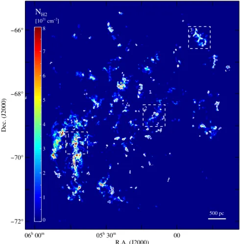
Figure 2. H2column density(NH2)map of the LMC at∼5 pc resolution(θ=20″, 1 beam per pixel sampling)produced by modeling the dust continuum emission
from Herschel100, 160, 250, and 350μm observations from HERITAGE (Meixner et al. 2013)using a modified blackbody. The white contours show the 1.2 K km s−1(3σ)and 5 K km s−1levels of the MAGMA DR3 CO map(θ=40″), which covered regions with prior CO detection. Assuming a Galactic conversion
factor ofXCO=2×1020cm−2(K km s−1)−1, the contour levels correspond to column densities of 2.4×1020cm−2and 1×1021cm−2. The dashed white boxes
indicate the three regions in Figure4. There is excellent agreement between the dust-based molecular gas map and the CO map even though the CO is not directly used to produce the map.
Following Leroy et al. (2009)and Bolatto et al.(2011), we model the dust emission in order to obtain the optical depth of the dust emission at 160μm(τ160). We use the results from two
different dust emission fitting techniques for the LMC, one presented in this paper and another from Gordon et al.(2014), both based on the assumption of modified blackbody emission,
( )
n
µ n b n
S B Td . We describe the fitting techniques in more
detail in Appendix A. For the SMC, we only produce one molecular gas map using the modeling results from Gordon et al. (2014)since Bolatto et al.(2011)produced a molecular gas map using afixedβsimple modified blackbody model and a similar methodology. The Gordon et al.(2014)dust modeling may produce a more accurate measure ofTdsince it allowsβto vary while reducing the amount of degeneracy betweenTdand β(Dupac et al.2003; Shetty et al.2009)by accounting for the correlated errors between the Herschelbands.
While the dust temperature along the line-of sight throughout the Magellanic Clouds likely has a distribution of temperatures (Bernard et al. 2008; Galliano et al. 2011; Galametz et al. 2013), the assumption of a single dust temperature on the small spatial scales we cover (∼20 pc)is reasonable since temperature mixing is restricted. Leroy et al. (2011)ran both simple modified blackbodyfits and more complex dust models from Draine & Li(2007)tofindτ160using theSpitzerdata for
the LMC and SMC, and found that both produced similar results. A future follow-up study of Gordon et al.(2014)will run more complex dust modeling of the HERITAGE
Herschel data.
This study focuses on using dust emission as a means to estimate the amount of molecular gas, which does not require a measurement of the dust mass. By only using τ160 we avoid
making any assumptions about the conversion to dust mass, which would introduce a further layer of uncertainty. We define our effective gas-to-dust(dGDR)ratio in terms ofτ160,
dGDR= SHI t160,
such that any proportionality constant between the IR intensity andτ160will be incorporated intodGDRand not affect ourfinal
results.
We expect, in principle, that the relationship between NHI
and τ160should go through the origin, but our measurements
show indications of an offset(see Figure1). We regionallyfit and then remove the offset and find that the relationship has a positive and roughly constant offset in NHI in both the LMC
(NHI~4´1020 cm− 2)
and SMC(NHI~1.5´1021 cm− 2)
. A similar offset was observed by Leroy et al. (2011), Bolatto et al. (2011), and Roman-Duval et al. (2014). As opposed to Bolatto et al. (2011), we remove the offset to avoid overestimates when creating maps of the gas-to-dust ratios, which would result in higher estimates of the total amount of gas. This offset could be due to a layer of HIgas with little to no dust, it could be due to the issues with background subtraction with theHerschelimages(particularly in the LMC where the HERITAGE maps to not extend much past the main part of the galaxy), or some combination of the two effects. Another possibility is that the relationship between NHI and
τ160is nonlinear and the slope(gas-to-dust ratio)decreases at
lowNHI, which we explore as part of the systematic uncertainty
estimation(see Sections3.1.1and4.1.2). Determining the true nature of the offset is beyond the scope of this work, but warrants further investigation. We subtract the offset in NHI
from the HImap and use the offset-subtracted map for the rest
of the analysis. For further discussion on the offset subtraction see AppendixB.
Steps to produce molecular gas map:
1. Model the dust emission in theHerschelimages to obtain τ160(see AppendixAfor more details).
2. Fit the HI offset in the NHI versus τ160 distribution
regionally(see AppendixBfor more details).
3. Produce first iteration map of the spatially varying effective gas-to-dust ratio (dGDR) at 500 pc scales
determined from the diffuse regions(Sgas= SHI)
a. ComputedGDR for each pixel.
b. Mask all pixels that likely have molecular gas: all regions within 2′of bright CO emission (ICO>3σ).
c. Use averaging of nearest neighbors to iterativelyfill in the masked (molecular)regions in the map.
d. Convolve map with symmetric Gaussian with FWHM=500 pc.
4. Estimate Smol using the first iteration of the smoothed
effectivedGDR:
(d )
Smol = GDRSdust - SHI.
5. Produce second iteration of map of spatially varyingdGDR
smoothed to 500 pc. Same as step 4 with the modification that both regions within 2′ of bright CO emission (ICO > 3σ) and points that have estimated
Smol >0.5SHIare masked.
6. Producefinal map ofSmolmap using the second iteration
of the smootheddGDR map.
Thefinal steps in producing the molecular gas maps remove unphysical artifacts. First, we remove small regions of estimated H2 that are likely spurious by masking pixels that have positive molecular gas in less than 50% of the pixels surrounding them within a 4′×4′box (12×12 pixels in the modified blackbody map from this work and 4×4 pixels in the maps from Gordon et al.(2014);∼60×60 pc in the LMC and ∼70 ×70 pc in the SMC). Generally, this removes emission smaller than∼2′(r∼ 30 pc in the LMC andr∼35 pc in the SMC)–two times the beam size of the lower resolution HIdata
—and regions of negative values (from underestimated total gas). Second, we median-filter the map over 3 pixels(∼1′in the LMC map from this work) to smooth out theSmol map and
remove spikes that are unphysical and below the resolution of the HI map, largely due to the residual striping from the HERITAGE PACS images(Meixner et al.2013).
There are a few caveats to this methodology that can potentially bias our molecular gas estimate. In addition to tracing the molecular gas (including any “CO-faint” comp-onent), our methodology may also trace optically thick and/or cold HI gas that emits disproportionately to the optically thin HI. Stanimirovićet al. (1999)takes a statistical approach and estimates the optical depth correction in the SMC based on column density using the absorption line measurements from Dickey et al.(2000)andfinds the correction only changes the total HI mass by ∼10%. Lee et al. (2015b) takes a similar approach to estimate an optical depth correction in the Milky Way andfinds that the correction only increases the mass of HI in the Perseus molecular cloud by ∼10%. Braun (2012) attempted to measure the HI optical depth from the flattening of the line profile in M31, M33, and the LMC, and found non-negligible optical depth corrections for high column densities (22<log NHI<23) in compact (∼100 pc) regions, which
estimate relies on the assumption of Gaussian line profiles to look forflattening of the HIline due to optical depth, which is a difficult measurement in the low S/N data. McKee et al. (2015) find ∼30% to be the appropriate HI optical depth correction for the solar neighborhood based on the average correction factors found using absorption line measurements in the plane of the Milky Way. Fukui et al. (2015), on the other hand,find more extreme opacity correction factors, as high as a factor of∼2 in the plane of the Milky Way using a relationship between NHI and the optical depth at 353 GHz from Planck.
The possible HIopacity corrections coming from a variety of methods and data show that the factors are uncertain.
The manner in which the optical depth correction will affect our molecular gas estimates is complex. It can increase the HI column density in the regions used to estimate the gas-to-dust ratio, leading to an increase in the total gas estimated in the molecular regions, and/or in the molecular regions, resulting in a decrease in the amount of molecular gas. We choose to use the HI statistical opacity corrections from Stanimirovićet al. (1999) and Lee et al. (2015b) to explore how correcting for optical depth effects our methodology in Section 4.1.3.
We note that, in Perseus where the structure of the molecular cloud is resolved, Lee et al.(2015b)compares their map of HI with the statistical optical depth correction to their inferred
“CO-faint” gas, observing that the structures are not spatially coincident(see Figure 4and Lee et al. 2015b). This suggests that the“CO-faint”gas cannot be explained by optically thick HI alone. Additionally, Lee et al.(2015b)comment that their opacity corrected HI map does not show the the sharp peaks seen in maps from Braun(2012).
Our methodology also relies on the assumption that the gas-to-dust ratio in the diffuse, atomic gas is the same in the molecular regions; we only measure the relationship between gas and dust in the atomic phase. There is observational evidence that the gas-to-dust ratio may vary from the diffuse to the dense gas in the Magellanic Clouds (Bot et al. 2004; Roman-Duval et al. 2014). In the Milky Way, Planck results show an factor of 2 increase in the far-IR dust optical depth per unit column density(τ250/NH)from the diffuse to the dense gas
(Planck Collaboration et al.2011), which would could indicate a lower gas-to-dust ratio in the dense gas. Both optically thick
HIand a decrease in the gas-to-dust ratio from the diffuse to the dense gas would mimic the effect of molecular gas and would result in our methodology overestimating the amount of molecular gas. We explore how these factors could affect our measurement ofH2in our systematic uncertainty estimate.
3.1.1. Map Sensitivity and Uncertainty
We use a Monte Carlo method to estimate the uncertainty in our molecular gas maps and determine the sensitivity levels. For the maps produced with the dustfitting from this work, we select three sub-regions (shown in Figure 2) with different levels of molecular gas (high, moderate, and low). We add normally distributed noise with an amplitude equal to the uncertainty to each of theHerschelbands andfitTdfor afixed β for each sub-region and then calculate τ160. For the dust
modeling results from Gordon et al.(2014), we add normally distributed noise to the τ160maps with an amplitude equal to
the uncertainty estimates from Gordon et al.(2014). Finally, we add noise to the HI map and create new Smol maps. The
process is repeated 100 times for each of the different maps. We use the distribution ofSmol for each pixel from the Monte
Carlo realizations to estimate a realistic uncertainty. The sensitivity of the maps is estimated byfinding the lowestSmol
that is consistently recovered at 2σ.
We know that the systematic uncertainty from the metho-dology will dominate the uncertainty in our molecular gas maps(Leroy et al.2009; Bolatto et al.2011). To estimate the level of systematic uncertainty, we see how changes to various aspect of the mapping methodology affect the estimated total molecular mass Mmol (which includes the factor of 1.4 to
account for He). We explore the effects of different assump-tions in the dust modeling and determination of the gas-to-dust ratio, and produces map that:
1. change the value ofβin our dust modeling and re-run the fitting with β=1.5 and β=2.0;
2. do not remove an HIoffset, which explores the idea that the relationship betweenNHIand τ160may not be linear
at low column densities; Table 1
Total Molecular Gas Mass Estimates for the LMC and SMC
Data Dust Fittinga Method Mmol[107M☉]b
LMC
1 Herschel 100–350μm MBB,β=1.8 dGDRmapc 9.9
2 Herschel 100–500μm BEMBB, 0.8<β<2.5 dGDRmapc 6.3
3 Herschel 100–350μm MBB,β=1.5 dGDRmapc 6.8
4 Herschel 100–350μm MBB,β=2.0 dGDRmapc 10.1
5 Herschel 100–500μm BEMBB, 0.8<β<2.5 dGDRmapc, no HIoffset 13.4
6 Herschel 100–500μm BEMBB, 0.8<β<2.5 GDR=540d 3.9
7 Herschel 100–350μm MBB,β=1.8 dGDRmapc,dGDR,dense=0.5dGDR,map 4.5
8 Herschel 100–500μm BEMBB, 0.8<β<2.5 dGDRmapc,dGDR,dense=0.5dGDR,map 4.0
SMC
9 Herschel 100–500μm BEMBB, 0.8<β<2.5 dGDRmapc 2.0
Notes.
a
MBB=modified blackbody, BEMBB=broken emissivity modified blackbody.
b
AssumingdLMC=50 kpc anddSMC=62 kpc.
c
Map of spatially varyingdGDR, see Section3.1. d
3. apply a single gas-to-dust ratio using the high and low values from Roman-Duval et al. (2014) (as opposed to using the map ofdGDR);
4. scale thedGDRmap down by a factor of 2 in the molecular
regions to account for a possible change in the gas-to-dust ratio from the diffuse to the dense gas, where we define the dense gas as regions in the map that are likely to have molecular gas(step 5 in Section3.1);
5. apply a single gas-to-dust ratio for the diffuse gas and a lower value for the dense gas using the values from Roman-Duval et al.(2014), where the dense gas value is applied to regions with bright CO emission(as in Roman-Duval et al. 2014).
For the versions of the maps where we use gas-to-dust ratios found in Roman-Duval et al.(2014), we use the maps ofSdust
in place ofτ160. We use the range inMmolvalues to estimate the
amount of systematic uncertainty in our molecular gas estimate.
3.1.2. Estimating H2from CO
For the purposes of this work, we want to compare the amount ofH2 traced by detected, bright 12CO emission to the molecular gas traced by the dust emission. To convert the CO intensity (ICO) into column density of mass, we use the
following equations:
( )= ( )
N H2 XCO COI 1
( )
a
=
Mmol COLCO, 2
where proportionality constants appropriate for Galactic gas are
XCO=2×1020cm−2(K km s−1)−1andaCO=4.3 M☉(K km
s−1pc2)−1, ICO is the integrated intensity of the 12CO
=
J 1 0transition(in K km s−1), andLCOis the luminosity
of the same transition(in K km s−1pc2). On small spatial scales and in CO-bright regions, using the Galactic values is a good approximation (Bolatto et al.2008).
3.2. Tracing Recent Star Formation
We use Ha, locally corrected for extinction using 24μm emission, to trace the star formation rate surface density(ΣSFR).
Following Bolatto et al.(2011), we use the star formation rate calibration by Calzetti et al.(2007)to convertHaand 24μm
luminosities:
( ) [ ( )
( ) ( )] ( )
☉ a
m
= ´
+
-
-M L
L
SFR yr 5.3 10 H
0.031 0.006 24 m , 3
1 42
where luminosities are in erg s−1andL(24μm)is expressed as νL(ν). The average contribution from 24μm to the total star formation rate is∼20% in the LMC and∼10% in the SMC. A significant fraction (∼40%) of the Ha emission in both the LMC and SMC is diffuse. We include all of theHaemission in this analysis since Pellegrini et al.(2012)showed that all of the ionizing photons could have originated from HIIregions from massive stars(see AppendixCfor further discussion). The rms background value of the star formation rate map is 1 × 10⁻⁴ M☉yr-1kpc-2 in the LMC and
4×10⁻⁴ M☉yr-1kpc-2 in the SMC.
This conversion to star formation rate assumes an underlying broken power-law Kroupa initial mass function(IMF)and was calibrated against Paschen-α emission for individual star-forming regions. Ideally,Haand 24μm emission would only be used for size scales that fully sample the IMF and sustain star formation for >10 Myr; for smaller scales, pre-main sequence stars are more appropriate and a better indicator of the current star formation rate. Hony et al. (2015)found that the star formation rate from pre-main sequence stars matches that fromHaat scales of ∼150 pc in the N66 region in the SMC. Our highest resolution of∼20 pc resolves HIIregions, and the mapping of the star formation rate on these scales is questionable. Nonetheless, we apply the star formation rate conversion even to our highest resolution data to allow us to compare to other studies and investigate the relationships in terms of a physical quantity, although it is important to keep these limitations in mind when interpreting the results.
3.3. Convolving to Lower Resolutions
To produce the lower resolution molecular gas maps, wefirst convolve the maps from theHerschelbeam to a Gaussian with FWHM of 30″for theβ=1.8 map(appropriate for the 350μm image resolution)and 40″for the BEMBB map(appropriate for the 500μm image resolution) using the kernels from Aniano et al.(2011). We then produce the range of lower resolution maps (from 20 pc to ∼1 kpc) by convolving the images of SSFR, Smol, and SHI with a Gaussian kernel with FWHM
( )
= r2-r
0
2 , whereris the desired resolution and r 0is the
starting resolution of the image. The images are then resampled to have approximately independent pixels (one pixel per resolution element). To mitigate edge effects from the convolution, we remove the outer two pixels(two beams)for all resolution images of the LMC. In the SMC, we remove two outer pixels for r 600 pc and remove one pixel from the edges forr 700 pc due to the small size of the images.
4. RESULTS
4.1. Molecular Gas in the Magellanic Clouds
Wefind molecular gas fractions that are comparable to the Milky Way in the LMC (17%), but much lower in the SMC (3%). These molecular gas fractions come from our new estimates of the total molecular gas mass: we find a total molecular gas mass (including He) in the LMC of
= -+ ´
MLMCmol 6.3 3.26.3 107 M☉ and MSMCmol =1.3-+0.651.3 ´107 M☉
Table 2 Global Properties
Property LMC SMC
Mmoldust 6.3-+3.26.3´107 M☉ 2.0-+1.02.0´107 M☉
LCO 7×10⁶K km s−1a 1.7×10⁵K km s−1b
MHI 4.8×10⁸ M☉c 3.8×10⁸ M☉d
*
M 2×10⁹
☉
M e 3×10⁸
☉ M f
SFRd 0.20 M☉yr−1 0.033 M☉yr−1
tdepmol 0.37-+0.190.37Gyr 0.61-+0.310.61Gyr
Notes.
a
Fukui et al.(2008), no sensitivity cuts.
b
Mizuno et al.(2001), no sensitivity cuts.
c
Staveley-Smith et al.(2003).
d
Stanimirovićet al.(1999).
e
Skibba et al.(2012).
f
in the SMC. These values are the sums(with no cuts) of our fiducial molecular gas maps that use the broken emissivity modified blackbody (BEMBB) dust modeling results from Gordon et al.(2014)with a spatially varyingdGDRand include
a factor of 2 systematic uncertainty. Table1 shows the results from our exploration of varying the map making methodology to estimate the systematic uncertainty combined with estimates of the molecular gas mass from the literature. In Table2we list the integrated properties of both galaxies. The molecular gas maps are sensitive toSmol ~15 M☉pc-2 (∼7 ×1020 cm−2)
based on the Monte Carlo estimates, which is comparable to the sensitivity of the SMC map from Bolatto et al. (2011). Our molecular gas fraction in the SMC is lower than previous estimates (Leroy et al. 2007; Bolatto et al. 2011), but is consistent with the factor of ∼2 estimate of systematic uncertainty for all of the estimates(see AppendixDfor further discussion).
Thefiducial molecular gas maps(β=1.8, broken emissivity modified blackbody(BEMBB)dust modeling)were produced using maps of the effective dust-to-gas ratio (dGDR) that had
average values for NHI t160 of 1.8±0.6×10 25
cm−2(LMC β =1.8), 1.3±0.3×1025cm−2(LMC BEMBB), and 4.8± 0.9 ×1025cm−2(SMC BEMBB). In the Milky Way, Planck Collaboration et al.(2014)foundNHI t160=1.1´1025cm−
2
in the diffuse ISM. OurNHI t160values are on average a factor
of∼1.5(LMC)and∼4.4(SMC)times higher than the diffuse Milky Way ISM, which is consistent with the expectation that the gas-to-dust ratio should increase with decreasing metallicity.
Given the total NANTEN CO luminosities of
( ) = ´
L COLMC 7 106K km s−1pc2 and L(CO)SMC=1.7´ 105K km s−1pc2 (using no sensitivity cuts), we find
a = -+
10 CO LMC
69 andaCOSMC=76-+3877, where all units forαCOare
given in M☉ (K km s−1pc2)−1. Compared to the Milky Way
value ofαCO=4.3(Bolatto et al.2013), the conversion factor
for the LMC is ∼2 times higher and the SMC is ∼17 times higher. OurαCOvalues are comparable to the dust-basedαCO
found by Leroy et al. (2011) of 6.6 (K km s−1pc2)−1 and 53–85(K km s−1pc2)−1for the LMC and SMC, respectively.
4.1.1. Structure of the Molecular Gas
One of the most striking results is the similarity of the structure of the molecular gas traced by dust to that traced by CO throughout the entire LMC(see Figures2and4)and SMC (see Figure3). Since our methodology only indirectly uses the CO map as a mask (see Section 3.1) the similarity is confirmation that our methodology traces the structure of the gas. Figure 4 shows that both dust modeling techniques produce maps with similar structure, although the BEMBB map tends to predict systematically lower amounts ofH2.
The details of the structures traced by CO are different from the dust-based molecular gas map. All of the regions shown in Figure4show molecular gas traced by dust, but not by CO at the 3σlevel. This is likely a layer of self-shieldedH2where CO has mostly dissociated, as expected from models(Wolfire et al. 2010; Glover & Mac Low2011). The same is generally true for the SMC, but having only the lower resolution full coverage NANTEN12CO map(r=2 6)makes detailed comparison of the structure difficult. Conversely, Region 2 in Figure4shows a molecular gas cloud traced by CO and not by the dust-based method. As discussed in Leroy et al. (2009), one possible explanation is that the dust is cold and faintly emitting in the far-IR, below the sensitivity of the HERITAGE Herschel
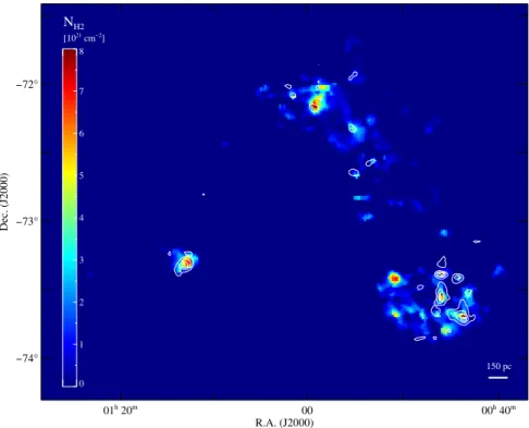
Figure 3.H2column density(NH2)map of the SMC at∼10 pc resolution(θ=40″, 1 beam per pixel sampling)produced by modeling the dust continuum emission
fromHerschel100, 160, 250, 350, and 500μm observations from HERITAGE(Meixner et al.2013)using the BEMBB dust modeling results from Gordon et al.
(2014). The white contours show the 0.45(3σ), 1, 1.5, and 2 K km s−1levels of the NANTEN CO map(θ=1′).
images. The peak in the CO emission of this cloud is detected from 250–500μm, but only weakly detected at 160μm and marginally detected (∼3σ) at 100μm, consistent with the interpretation of cold dust. There are a few other detections of CO without a dust-based molecular gas counterpart, although the cloud in Region 2 is the clearest example with the strongest CO emission.
4.1.2. Systematic Uncertainty
The systematic uncertainty comes from the different possible assumptions that can be made in the dust modeling and the method of measuring the gas-to-dust ratio. Because the statistical errors are typically small, the systematic uncertainty dominates the total uncertainty in the molecular gas mapping methodology (Leroy et al. 2009; Bolatto et al. 2011). We present the range of our total molecular gas mass estimates (Mmol)in Table1(we list allMmolestimates alongside estimates
from the literature in Table3in AppendixD). We use the range of as a means to gauge the amount of total systematic uncertainty and we look at the variation between the two fiducial molecular gas maps (Table 1 rows 1 and 2) with different dust modeling assumptions to determine the amount of systematic uncertainty due to assumptions in the dust modeling.
The two lowest Mmol estimates that we found use a single
gas-to-dust ratio of 380 from Roman-Duval et al. (2014)and
use the upper estimates for the gas-to-dust ratios for the diffuse and the dense gas from Roman-Duval et al. (2014) of GDRdiffuse=540 and GDRdense=330(see rows 6 and 10 in
Table 3 in Appendix D). These maps have large regions of negative values from where the estimated total gas is less than the HI, which causes only small areas of estimatedH2and the lowMmolvalues, which would be due to using too low a value
of the gas-to-dust ratio. The value forMmolwith GDR=380 is
less than the total molecular gas you would obtain by applying a Galactic CO-to-H2 conversion factor to the low resolution NANTEN CO map, which is a lower limit on the total molecular gas since a higher conversion factor should be appropriate when the CO structure is unresolved. We do not consider these values ofMmol when estimating the systematic
uncertainty in the total molecular gas mass.
The difference between the highest(row 5)and lowest(row 6) molecular gas mass is ∼3.5. The minimum Mmol estimate
(row 6)comes from assuming a single gas-to-dust ratio of 540, which is the highest value found by Roman-Duval et al.(2014). ThisMmol estimate is only a factor of∼1.5 lower than using a
spatially varying dGDR applied to the same BEMBB dust
modeling results. The maximum value comes from using the BEMBB modeling that does not remove an HIoffset(row 5), which allows for a possible nonlinear relationship in NHI
versusτ160(see Section3.1.1and AppendixB). This would be
an overestimate if the relationship betweenNHI versusτ160is
Figure 4.The top and bottom rows of images, respectively, show the enlarged regions of theNmolmaps(identified in Figure2)for the dust modeling withβ=1.8 and
the BEMBB model from Gordon et al.(2014)at the same color scale as show in Figure2. The contours show the MAGMA12CO intensity at levels of 0.6(3σ), 2, and 5 K km s−1with the dashed gray line showing the survey coverage in the regions. The white line on the color bar indicates the estimated sensitivity level of
~ ´
Nmol 7 1020cm−2(Smol~15 M☉pc-2). Both dust-based molecular gas maps show similar structure. The dust-based estimate tends to show more extended molecular gas than that traced by12CO. The only clear example of a CO cloud(with strong CO emission)with no dust-based molecular gas counterpart(in both the
linear since it will artificially increase thedGDR values in the
maps. Allowing for a difference in the gas-to-dust ratio in the diffuse and dense gas by scaling downdGDR in the dense gas
reduces Mmol by a factor of∼2 for theβ =1.8 map and∼1.5
for the BEMBB map. We conclude that our molecular gas estimate is good to within a factor of∼2, which agrees with the estimates from similar methodologies by Leroy et al. (2009, 2011)and Bolatto et al.(2011).
We compare the effects of different dust modeling techniques by usingβ=1.8 and BEMBB maps while keeping all other aspects of the methodology the same(using a spatially varying dGDR). Figure 4 shows the difference between the
molecular gas maps using theβ=1.8 and BEMBB modeling (top and bottom rows, respectively). The BEMBB map is a factor of∼2 lower for molecular gas column density estimates than using the fits from theβ =1.8 model. The difference in values between the two maps shows no variation as a function of τ160, which indicates that the dust models do not produce
systematically different results in the dense gas as compared to the diffuse. The τ160 values from the BEMBB modeling
(Gordon et al.2014)tend to be higher than from theβ =1.8 modeling, largely due to differences in the fitted dust temperatures (Td). The BEMBB modeling tends to fit higher
Td, which is a result of the range ofβvalues combined with the degeneracy betweenβand Td(Dupac et al.2003; Shetty et al. 2009):fitting a lowerβvalue to the same data will result in an increase in Td. An increase in τ160 produces lower effective
gas-to-dust ratio (dGDR)and a lower estimate of the amount of
molecular gas. Our adopted factor of∼2 systematic uncertainty is consistent with the variation seen between the two maps.
4.1.3. Estimating the Effect of the Optical Depth of HI
We apply the statistical optical depth corrections from Stanimirovićet al.(1999)for the SMC and Lee et al.(2015b) for the Milky Way toNHImaps to estimate how accounting for
optically thick HI could affect our molecular gas estimate. There is no comparable optical depth correction for the LMC, so we apply the statistical corrections for the lower metallicity SMC and higher metallicity Milky Way to estimate a range of possible effects. Applying the Lee et al. (2015b)correction to the LMC HIproduces a maximum correction factor of 1.43 and shifts the top 5% of NHI from >3.1 × 10
21cm−2 to
>4.0 × 1021cm−2, whereas the Stanimirović et al. (1999) correction produces a maximum correction factor of 1.36 and shifts the top 5% to >3.3 × 1021cm−2. Applying the Stanimirović et al. (1999) correction to the SMC produces a maximum correction factor of 1.48 and shifts the top 5% of the
NHI from >4.4 × 10
21cm−2 to >5.2 × 1021cm−2. In the
LMC, both of the statistical optical depth corrections decrease the total molecular gas mass estimate by ∼5% while in the SMC it increases the total molecular gas mass by a factor of ∼2, both are within our estimate of the systematic uncertainty. The molecular gas estimate changes because the amount of HIin the diffuse regions, where we determine the effective gas-to-dust ratio, increases or decreases with respect to the amount of HIin the molecular regions. Optical depth corrections in the diffuse gas will increase the effective gas-to-dust ratio and increase the estimate of the total amount of gas. If the optical depth corrections in the molecular regions are similar to the corrections in the diffuse regions, as is the case in the SMC, the total amount of gas will increase and the molecular gas estimate will increase. If the optical depth corrections in the molecular
regions are larger than in the diffuse, more of the total gas estimate will be due to HIas opposed toH2and the molecular gas estimate will decrease, as is the case in the LMC. Ultimately, the decrease in the molecular gas mass estimate in the LMC is negligible, which indicates that optical depth effects do not significantly contribute to our molecular gas estimate.
4.1.4. Comparison to Previous Work
The molecular gas maps we present are improvements upon previous dust-basedH2 estimates given the availability of the
Herschel data with increased sensitivity and coverage of the far-IR combined with improvements in the methodology and more extensive estimation of the systematic uncertainty. Table1 includes the existing dust-based molecular gas mass estimates for LMC and SMC from the literature. While some of the total molecular mass values are outside the range of the estimate from this work, they can all be reconciled and explained by differences in methodology and limitations in the data. For a more detailed explanation of the differences in the Mmol
estimates from previous works see AppendixD.
4.2. Molecular Gas and Star Formation
Understanding whether or not metallicity and galaxy mass affect the conversion of gas into stars is important for understanding galaxy evolution throughout cosmic time. The relationship between molecular gas and star formation rate has been studied extensively in nearby, high-metallicity, star-forming galaxies. With the dust-based molecular gas estimates of the nearby Magellanic Clouds, we are in a unique position to probe how the relationship between the molecular gas and star formation rate behave as a function of metallicity and the size scale considered. Figure5shows the relationships for the LMC and SMC using the new dust-based molecular map at the highest resolution of 20 pc, 200 pc (the scale where multiple star-forming regions are being averaged), and 1 kpc( compar-able to the12CO surveys of nearby galaxies).
We compare the relationship between the molecular gas and the star formation rate in the SMC and LMC to that for the HERACLES sample of nearby galaxies by Leroy et al. (2013b). The HERACLES sample resolves the galaxies and compares the gas and star formation at a resolution of∼1 kpc. Figure6 shows that the LMC and SMC data(convolved to a comparable resolution of 1 kpc)lie within the scatter in the data for high-metallicity, star-forming galaxies, although above the main cluster of data points for a given molecular gas surface density.
4.2.1. Molecular Gas Depletion Time
A convenient way to quantify the relationship between molecular gas and star formation is in terms of the amount of time it would take to deplete the current reservoir of gas given the current rate of star formation, the molecular gas depletion time:
( )
tdep = S S . 4
mol
mol SFR
molecular gas mass and star formation rate does not significantly affect the averages at 1 kpc scales; at 200 pc scales, weighting of the average typically changes the value of tdepmolby∼20%. The main exception is for the star formation rate
weightedtdepmolaverage in the LMC, which is shorter by∼50% and likely due to the significant contribution of 30 Doradus at these scales. The range of possible molecular gas depletion times given the factor of up to∼2 systematic uncertainty in the molecular gas estimate is∼0.2–1.2 Gyr. This is shorter than the molecular gas depletion time found for the SMC by Bolatto et al. (2011)of tdep ~1.6
mol Gyr at 1 kpc resolution, but within
the factor of 2 systematic uncertainty on both estimates. The molecular gas depletion time found in the Magellanic Clouds is lower than the average value of∼2 Gyr for nearby normal disk galaxies at comparable∼1 kpc size scales, but within the range of observed values for the STING sample(Rahman et al.2012) and the larger HERACLES sample (Bigiel et al. 2008,2011; Leroy et al. 2013b).
Figure 7 shows that the median tdep mol
is ∼2–3 Gyr at the highest resolution of 20 pc. The molecular gas depletion time changes with resolution because the peaks in the molecular gas are physically separated from the peaks in the star formation rate at scales where the star-forming regions are spatially resolved. The tendency of low star formation rates at the peaks in the molecular gas, and low to no molecular gas at the peaks in the star formation rate(tdepmolis only defined for regions with Smol) biases tdepmol at high resolutions toward longer times. A
scale of 200 pc is typically large enough to include both the recent star formation and the molecular gas and sample star-forming regions at a range of evolution stages (Schruba et al.2011). While the molecular gas depletion time gets closer to the integrated tdepmol value at a scale of 200 pc, the median
tdepmol reaches the integrated value at ∼500 pc in the LMC
and SMC.
The lower metallicities of the SMC and LMC and the lack of a metallicity bias in our dust-based molecular gas estimate allow us to investigate whether there is any trend intdepmol with
metallicity. Figure9 shows that there is no clear trend in the average molecular gas depletion times when comparing the LMC and SMC to the HERACLES sample of galaxies. Leroy et al.(2013b)also saw no trend with metallicity as long as they allowed for a variable CO-to-H2 conversion factor. We also compare our measurements to the integrated tdep
mol
using a metallicity-dependent CO-to-H2 conversion factor for the
Herschel Dwarf Galaxy Survey (DGS; Cormier et al. 2014). Over the range of metallicities studied, the main cause of variations in the molecular gas depletion time does not appear to be metallicity.
4.3. Correlation Between Gas and Star Formation Rate from 20 pc to 1 kpc Size Scales
We use the Spearman’s rank correlation coefficient to quantitatively gauge how well the gas correlates with star formation rate at different size scales. Spearman’s rank correlation coefficient (rs) measures the degree to which two quantities monotonically increase(rs>0)or decrease(rs<0). We computed the 3σ confidence intervals using the Fisher z -transformation, which is appropriate for bivariate normal distributions. Figure 8 shows the rank correlation coefficient as a function of resolution for the relationship between star formation rate and molecular gas and atomic gas.
The change in the rank correlation coefficient with resolution is similar for both the LMC and SMC. As expected for atomic-dominated galaxies, the correlation ofSgasversusSSFRfollows
that ofSHIandSSFR, therefore we only showSHIversusSSFR
in Figure8. The correlation betweenSHI versusSSFR in both
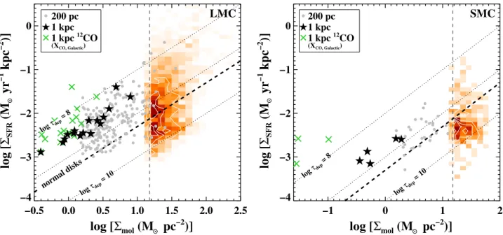
Figure 5. SSFRas a function ofSmolfor the LMC(left)and SMC(right)at various resolutions. The red color scale shows the two-dimensional distribution at a
resolution ofr=20 pc while the white contours indicate levels that are 20%, 40%, 60%, and 80% of the maximum density of points. The vertical gray dashed line indicates the estimated 2σsensitivity cut of ther=20 pc data(Smol~15M☉pc-2). The gray circles and black stars show the data at resolutions ofr=200 pc and
r=1 kpc, respectively. The green stars showSmolderived from NANTEN CO data at a resolute ofr=1 kpc using a Galactic CO-to-H2conversion factor. Here we
the LMC and SMC is high (rs ∼ 0.6–0.7) at the smallest size scale of 20 pc and remains high across all size scales. The correlation of HI with the star formation rate, even at small spatial scales, is due to the extended nature of both components combined with the general trend that regions with more total gas have more star formation and more molecular gas.
The SH2 versus SSFR distribution reaches the maximum
correlation coefficient ofrs∼0.9 at a size scales∼200 pc, past which it is better correlated than the relationship with HI. While the HI is correlated with the star formation rate tracer, we see that molecular gas is best correlated with recent star formation in the LMC and SMC at size scales 200 pc. The 200 pc scale indicates the average size scale where both molecular gas and the star formation rate tracer,Ha, are found together and enough independent star-forming regions at different evolutionary stages (i.e., different ratios of Ha to molecular gas) are averaged together. While the correlation peaks at 200 pc, the average molecular gas depletion time decreases until it reaches the integrated value at a size scale of ∼500–700 pc in the LMC and SMC. The molecular gas and star formation rate tracer have a strong positive correlation, stronger than that with HI, supporting the physical connection between molecular gas and recent massive star formation.
5. DISCUSSION
We discuss ourfindings on the relationship between gas and star formation in the Magellanic Clouds using our new dust-based molecular gas maps. By comparing our results to existing observational studies of mainly massive, high-metallicity, molecular-dominated galaxies, simulations, and theoretical models of star formation, we provide insight into the physical mechanisms that drive star formation.
5.1.tdepmol in the Magellanic Clouds
The range of possible molecular gas depletion times for the LMC and SMC at 1 kpc scales given the systematic uncertainty in our estimate of the molecular gas of ∼0.2–1.2 Gyr falls below the average ∼2 Gyr found for nearby normal disk galaxies. This is consistent with the previous work by Bolatto et al. (2011)that found tdep =1.6 Gyr
mol at 1 kpc scales in the
SMC using similar dust-based molecular gas estimates, with the value being higher due to a higher estimate of the molecular gas. The shorter molecular gas depletion times do not appear to be directly due the lower metallicities as there is no trend in tdepmol with metallicity(see Figure9).
The other remaining environmental factors, besides metalli-city, that could affect the ratio of the amount of molecular gas to the amount of current star formation are the lower galaxy masses of the Magellanic Clouds and the interaction between the LMC, SMC, and Milky Way (Besla et al. 2012). Lower mass galaxies tend to have lower dark matter and stellar densities, making them more susceptible to stochastic bursts of star formation. Both the star formation histories of the SMC and LMC (Harris & Zaritsky 2004, 2009) indicate that there have been recent bursts in star formation in both galaxies. A burst in star formation over a short period of time could lead to a depletion of the molecular gas reservoir combined with higher star formation rates that together can produce lowtdepmol values.
The molecular gas depletion time in M33 is∼0.5 Gyr when the diffuse Ha emission is included (Schruba et al. 2010), which is comparable to our measurements of the Magellanic Clouds. If the diffuse ionized gas(DIG) is removed from the
a
H emission, then the molecular gas depletion time increases to∼1 Gyr. This highlights the importance of understanding the connection between the DIG and recent massive star formation as it represents a significant fraction of theHa emission and changestdepmol. Rahman et al.(2011)found a similar increase in tdepmol
by a factor of∼2 when the DIG was removed in the disk galaxy NGC 4254. If the diffuse ionized component is excluded in the star formation rate determination, the tdepmol in
M33, LMC, and SMC is∼1 Gyr. Figure 6.SSFRvs.Smolfor ther∼1 kpc data from the HERACLES sample of
nearby star-forming galaxies (Leroy et al.2013b) (blue), where theSmol is
estimated using12CO with a Galactic CO-to-H2 conversion factor. Ther∼
1 kpc data for the LMC(filled stars)and SMC(open stars)are over plotted. The LMC and SMC points fall within the full distribution for the HERACLES sample, but offset above the main distribution.
Figure 7.Median molecular gas depletion time as a function of resolution. Blackfilled and open gray circles show the data for the LMC and SMC, respectively. The error bars show 1σon the mean. The upper dashed line shows
tdepmol=2 Gyr, the average for normal galaxies, and the lower dashed line showstdepmol=0.4 Gyr, the integrated depletion time for both the LMC and SMC. The LMC and SMCtdepmol reach the integrated value of∼0.4 Gyr and
Like the Magellanic Clouds, M33 is low-mass, atomic-dominated, and has likely interacted with M31 within the past 0.5–2 Gyr(Davidge & Puzia2011). The LMC, SMC, and M33 show evidence for bursts in the star formation history within the last Gyr and the most recent epochs show lower star formation rates, which suggest that the star-forming gas reservoir has been depleted. The observed shorter depletion times appear to be caused by catching these galaxies after a period of higher star formation rate and does not necessarily indicate that these low-mass, low-metallicity galaxies are forming stars differently from normal disk galaxies.
Saintonge et al. (2011) also found that for the volume-limited COLD GASS survey, lower stellar mass galaxies (∼1010M☉) had shorter depletion times of ∼0.5 Gyr. While
consistent with the integrated depletion times in the LMC and SMC, the data are not completely comparable since a value for the CO-to-H2 conversion factor has to be assumed and single-dish CO observations from the COLD GASS survey will mainly detect the central regions of the galaxies. Saintonge et al.(2011)conjecture that the shorter depletion time is due to the tendency for smaller galaxies to have more “bursty” star formation. Similarly, Cormier et al. (2014) suggest that the observed short molecular gas depletion depletion times for their DGS sample of dwarf galaxies are due to recent bursts in star formation. Kauffmann et al. (2003) found that low redshift galaxies with stellar mass<3×10¹⁰ M☉in the Sloan Digital
Sky Survey have younger stellar populations and that the star formation histories are correlated with the stellar surface density, also indicative of recent bursts in star formation as seen in the LMC, SMC, and M33. In Figure 10, we show the average tdepmol time as a function of the average stellar surface density(S*)for the LMC, SMC, and the HERACLES sample of galaxies and see that all of the low molecular depletion times are found at lowS*. The fact that low-mass galaxies are more susceptible to stochastic star formation can produce bursts in
star formation (Hopkins et al. 2014) and lead to shorter molecular gas depletion times.
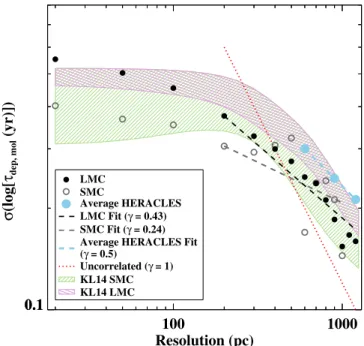
5.2. Physical Interpretation of the Scatter intdepmol
The scatter in theSmol–SSFRrelationship, which we quantify
in terms of the scatter in logtdepmol, can be produced by both
physical mechanisms and the imperfect nature of the observable tracers of the physical quantities. The previous observational work that focused on the scatter in tdepmol, or the “break down”of theSmol–SSFRrelationship, by Schruba et al.
(2010), Verley et al.(2010), and Onodera et al.(2010), studied theSmol - SSFRrelationship in M33 over100 pc size scales.
Schruba et al. (2010) compared tdepmol found for apertures
centered on CO peaks to apertures centered onHa peaks for various aperture sizes from 75 to 1200 pc and found that the tdepmol values differed for CO and a
H peaks for 300 pc size scales. There are a number of possible causes of the difference between the CO and Ha molecular gas depletions times: a difference in evolutionary stage of the star-forming region, drift of the young stars from their parent cloud, actual variation in tdepmol, differences in how the observables map to physics
quantities, and noise in the maps. Schruba et al.(2010)identify the evolution of individual star-forming regions as the likely cause for the variations.
At high resolution(scales of ∼20–50 pc), the star formation and molecular gas are resolved into discrete regions that span a range evolutionary stages(e.g., Kawamura et al.2009; Fukui & Kawamura2010)and have different ratios of molecular gas to star formation rate tracers. Averaging over larger size scales samples regions at a range of evolutionary stages resulting in a
“time-averaged” tdepmol. The change in the scatter in the
molecular gas depletion time (σ) with resolution informs us about whether the star-forming regions are spatially correlated due to synchronization of star formation by a large-scale Figure 8.The Spearman rank correlation coefficient(rs)as a function of image
resolution for theSH2 vs.SSFR (circles with solid line) andSHI vs.SSFR
(squares with dashed line) distributions. The top plot shows the rank correlations for the LMC and the bottom show those for the SMC. The error bars show the 99.75% confidence interval (∼3σ) of the measured rank correlation coefficient. The correlation between HIand the star formation rate
remains at a constant, high level ofrs∼0.7 across size scales in part due to the
extended nature of both the HIgas andHaemission that dominates the star formation rate. The correlation betweenH2and star formation rate reaches a
maximum value ofrs∼0.9 at a size scale of 200 pc, which is the expected size
scale to average over enough individual star-forming regions to sample a range of evolutionary states.
Figure 9.The galaxy-averaged molecular gas depletion time(áS ñ áSmol SFRñ)
with metallicity for the HERACLES sample(light blue points), LMC(black
filled stars), and SMC(gray open stars). We have taken the averageSmoland
SSFRof the 1 kpc LMC and SMC data, which are comparable measurements to
the ∼1 kpc resolution HERACLES data. We also include the integrated molecular gas depletion times (M(H2) star formation rate) from the DGS using a metallicity-dependent CO-to-H2conversion factor from Cormier et al.