A LOW-ENERGY STUDY OF THE20Ne(p, γ)21Na REACTION WITH HIGH-CURRENT PROTON BEAMS AT LENA
Andrew Leland Cooper
A dissertation submitted to the faculty at the University of North Carolina at Chapel Hill in partial fulfillment of the requirements for the degree of Doctor of Philosophy in the Department of Physics.
Chapel Hill 2019
Approved by:
c
O2019
ABSTRACT
Andrew Leland Cooper: A Low-Energy Study of the 20Ne(p, γ)21Na Reaction with High-Current Proton Beams at LENA
(Under the direction of Arthur E. Champagne)
The neon-sodium (NeNa) cycle is believed to play a pivotal role in explaining the oxygen-sodium abun-dance anticorrelation exhibited by members of all carefully observed globular clusters, but not seen in field stars. High-current, low-energy cross section measurements of the20Ne(p,γ)21Na reaction at the Laboratory for Experimental Nuclear Astrophysics (LENA) can clarify the rate at which the NeNa cycle occurs and enhance our understanding of stellar nucleosynthesis in the globular cluster environment. However, the pri-mary challenge in directly measuring nuclear reaction rates at stellar energies is their extraordinarily small cross sections (often< 10−9 b). When combined with novel detection techniques, this hurdle can be over-come by employing high-current (mA-range), pulsed proton beams from the electron cyclotron resonance ion source (ECRIS) at LENA. Development and performance highlights of this system are described. This ion source also provided low-energy 20Ne+ beams to implant the necessary tantalum and titanium targets for this experiment. Target stoichiometries were measured via nuclear reaction and Rutherford backscattering analyses. A lead-shielded, dual, high-purity germanium detector arrangement in a 55◦-90◦ geometry was constructed for this experiment to minimize angular correlation and Doppler-shift effects within collected spectra. This detection system was characterized using Monte Carlo-based simulations inGEANT4. Ex-perimental results from recent measurements of the strength and primary decay branching ratios of the Elab r
= 384-keV resonance in20Ne(p,γ)21Na at LENA are given. Also, a measurement of the total cross section at Elab
ACKNOWLEDGEMENTS
My graduate career at the University of North Carolina (UNC) at Chapel Hill has been the most chal-lenging, productive, and rewarding period in my life. I firmly believe that I would not have been nearly as successful without my wonderful colleagues at the Laboratory for Experimental Nuclear Astrophysics (LENA) at the Triangle Universities Nuclear Laboratory (TUNL), who taught me many things along the way. Likewise, I do not believe that I would have survived this journey without love and support of my wife, family, and close friends. Hence, I wish to take a moment to acknowledge their contributions and thank them individually.
Dr. Thomas B. Clegg was the first person that I connected with at UNC. His action-packed, prospective student tour of LENA and TUNL is what first reeled me into working in nuclear astrophysics, having had no prior experience in nuclear physics. Once I got to know Tom and his science interests, I realized that working with him at LENA was the right fit for me. Tom taught me how to defend what I thought was right, think fast on my feet, and never fear being wrong. He taught me how to break projects down into manageable pieces and that no challenge is insurmountable with dedication and hard work, no matter how impossible or large it might seem. In short, Tom gave me the professional confidence that a successful scientist requires. Along with these personal lessons, I learned the technical and historical details of high-intensity ion source development from one of its masters. In science (experimental nuclear physics, especially), one needs allies
−Tom has no shortage of them because of his personable attitude that treats others, from all walks of life, with respect and a smile. Because of this, I thank Tom for his willingness to give a working-class, relatively-average student like myself the educational opportunity of a lifetime.
hand. I thank Art for his individuality, his experimental and career advice, and for the research opportunities described in this text.
During my stay at UNC, I was fortunate to have chosen great members for both my master’s and doc-toral degree committees. I was lucky to have Dr. Robert Janssens join our lab and my committee. He has an incredibly diverse background, and was an exceptional source of knowledge and assistance concerning experimental setup and detector diagnostics. His hospitality and positive attitude always made work much easier. I thank Dr. Richard Longland for serving on this committee and for his assistance with data collection with the tandem accelerator at TUNL. Also, I thank Dr. Fabian Heitsch for serving on this committee and providing an astronomer’s perspective at the discussion table. Dr. Reyco Henning served on my master’s committee and I thank him for always having a genuine interest in my current research endeavors−a kind word in the hall from him always made a big difference.
I also benefited from research opportunities and advice given by folks who were not on my degree com-mittees. I thank my undergraduate advisor, Dr. Daniel H. McIntosh, for giving me my first research job in astrophysics and demonstrating how to stay true to one’s roots in their professional life. Also, I thank Dr. Christian Iliadis for his instruction in nuclear astrophysics and input on experimental setup.
My postdoctoral colleagues at TUNL have set the standard to which I aspire following my departure. Dr. Chris Howard was a significant resource for me upon my arrival at LENA, since I knew almost nothing about nuclear experiments − I thank him for taking the time to introduce me to some of the basics. To say that Dr. Kiana Setoodehnia helped make the experiment described below happen would be a massive understatement. Through all of the tandem accelerator’s beam instabilities and detection system issues during this experiment, Kiana soldiered on with me. Kiana is tough. When others would have left, Kiana stayed; when others would have given up, Kiana helped solve the problem at hand; when others would have gotten irritated, Kiana never complained. I thank her for this contribution and I sincerely hope that she finds more success and satisfaction after TUNL. Also, I thank Amber Lauer for her assistance with ECRIS repairs.
physically challenging; and he gladly collected data overnight for this experiment. Most importantly, Sean always exuded a positive attitude and was a great co-worker. We did it, Sean − we broke out of LENA. Lori Downen was also a huge help during data collection and setup for this experiment. Her delicious baked sweets kept everyone energized during long days in the control room. Also, her software troubleshooting and data analysis advice was very helpful. When it came to detector construction and simulation for this experiment, David Little was the undisputed master. The conversations that I had with him concerning GEANT4simulation ideas saved me a lot of time and his assistance with keeping the detectors cool while I was away was greatly appreciated. Dr. John “Jack” Dermigny provided valuable computational advice and software technical support. He was also very helpful in the early days of the ECRIS acceleration column upgrade while we were getting the extraction system stepper motor control software working and calibrated. I also want to thank Federico Portillo and Caleb Marshall for providing operational assistance at the tandem lab during this experiment. While he was still a UNC student at LENA, Dr. Keegan Kelly trained me in accelerator operation and other important laboratory skills. I thank him for being incredibly patient and helpful during the ECRIS column upgrade project. It was a pleasure to be instructed by him on how to operate the ECRIS, and I was glad we were able to provide him the accelerator he needed to collect his thesis data. I also thank Dr. Grayson Rich for his assistance with the installation of the high-power microwave system for the ECRIS. Dr. Thomas Corona assisted us during the beam optics simulation phase of the ECRIS column upgrade−I thank him for his help.
for this experiment, and I helped him with his target characterization project.
I always looked forward to working with the easy-going technicians at TUNL. Chris Westerfeldt, Richard O’Quinn, and John Dunham together taught me everything about high-voltage, high-power, beam transport, safety interlock, and radiation monitoring systems. At the outset of the ECRIS column upgrade project, I had, in essence, no practical, laboratory skills, aside from automobile and small-engine repair−working with Brian Walsh quickly changed that. He taught me basic plumbing, wiring, rigging, and other maintenance skills that I will use for the rest of my career. Working with Brian was sometimes frustrating or disgusting (depending on the job), but always amusing and productive −I hope he is doing well. Similarly, I had a basic knowledge of laboratory electronics prior to working at LENA−my spirited trial by fire came while working with Bret Carlin. Bret is truly the mastermind behind the software and hardware for the ECRIS LabView control system, along with the rest of the electronics that LENA relies on. It was always an exciting and rewarding experience working with him. I first met Mark Emamian after Jason Surbrook and I had finished our Autodesk Inventor concept drawings of the ECRIS column. Mark quality-checked and annotated these preliminary part drawings to prepare them for fabrication by the UNC Physics and Astronomy Instrument Shop. His dedication to working with Tom Clegg and I to get all of these parts correct was immensely appreciated. Also, I thank him for the hours spent training me in the fine art of surveying with an optical transit scope (a skill that I did not expect to learn prior to working at LENA), in order to get the alignment of electrode apertures within the ECRIS absolutely correct. Thanks to his woodworking background, Tom Calisto brought quick fabrication abilities, combined with practical maintenance skills, to LENA. This valuable combination was instrumental for conquering the countless beam line repairs and the construction of the lead-shielded target station necessary for this experiment.
For experimental nuclear physicists, dreams come true in the machine shop. The UNC Physics and Astronomy Instrument Shop completed the fabrication of the main electrodes and internal components of the ECRIS column. Cliff Tysor and Philip Thompson did a remarkable job at producing its precision metal and ceramic components on a tight schedule. The Duke University Instrument Shop served as a triage for machining jobs immediately following the installation of the ECRIS column and during beam line upgrades, and they also fabricated the lead-shielded target and detector station for this experiment. Bernie Jelinek, Phil Lewis, and Richard Nappi never turned down our numerous pop-up machining jobs (even on Friday afternoons)− I thank them for their time and efforts. I could not have asked for a nicer group of guys to work with and always looked forward to visiting the shop to talk about life with Bernie, stock car and truck racing with Phil, and astronomy with Richard.
DE-FG02-97ER41041 and DE-FG02-97ER41033). I also thank William Park, Geoff Ryding, and Noah Smick
−all researchers at Neutron Therapeutics−for their advice on the design and construction of the ECRIS column. Lastly, I thank Tony Mendez for his ECRIS beam optics simulations usingSIMION, whose results guided us to successful use of the fixed cone focusing electrode.
My journey to UNC and LENA would not have happened without the support of my family and friends. My dad, Marty, is the hardest working person I have ever known (a career truck driver with a million-mile safety record) and also one the easiest-going people, who makes friends wherever he goes. Thank you for imparting these personal traits onto me, Dad, and for always being eager to hear about what I have been working on. I thank my mom, Michelle, for instilling a love of learning in me, prioritizing my education from the time I was born, and inspiring me to go after my dreams (no matter how crazy they might seem). You sacrificed your time and opportunities in your own life for the benefit of mine. To my siblings Matthew, Amelia, William “Rusty”, and Alissa, thank you for welcoming me home each Christmas and 4th of July
−
watching you all grow into individuals with your own temperaments and dreams is one of the best things in life. My grandmother, Linda, has been my lifelong cheerleader. From the time I turned my eyes toward the night sky, she helped finance every new eyepiece, star chart, or telescope that I justhad to have. When it came to my love for science, she kept (and keeps) the fire burning. I thank Bradley Cooper, Mark Reynolds and the rest of his family, Justin Mann, and Jeff and Katelynn Treolo for providing the kind of friendships that many folks never get to experience, even at long-distance. I also thank Chloe, Gina, and Mike Shepard for their support and their eagerly-anticipated 4th of July celebrations each year.
TABLE OF CONTENTS
LIST OF TABLES . . . .xviii
LIST OF FIGURES . . . xix
LIST OF ABBREVIATIONS. . . .xxviii
1 Introduction . . . 1
1.1 Nuclear Astrophysics: The Crossroads of The Large and Small . . . 1
1.2 Not So Simple: Globular Clusters and the Oxygen-Sodium Anticorrelation. . . 2
1.2.1 Evolutionary Phases of Intermediate-mass GC Members . . . 3
1.2.2 GCs as Cosmic Laboratories . . . 5
1.2.3 Evidence and Formation Scenarios for Multiple Populations in GCs . . . 6
1.2.4 The TP-AGB Scenario: Stellar Physics Constraints and Motivations for New Cross Section Measurements . . . 10
1.3 Constraining Reaction Rates with Laboratory Measurements . . . 11
1.3.1 Experimental Yields and Cross Sections . . . 11
1.3.2 Nuclear Reaction Rates . . . 14
2 Beam Acceleration and Transport Systems at LENA . . . 16
2.1 Laboratory for Experimental Nuclear Astrophysics: Overview . . . 16
2.2 Modified 1-MeV Model JN Van de Graaff . . . 17
2.2.1 Basic Operation . . . 17
2.2.2 RF Ion Source . . . 19
2.3 Electron Cyclotron Resonance Ion Source at LENA. . . 20
2.3.1 Fundamentals of ECR Plasma Generation . . . 20
2.3.2 Design and Operation . . . 23
2.4.1 Analyzing Magnet . . . 26
2.4.2 Design and Placement of Magnetic Solenoid Lenses, Steerers, Quadrupoles, and High-Power Faraday Cups . . . 26
2.4.3 Target Station . . . 27
3 Advancements in Component Protection and Experimental Feasibility with High-Intensity, Pulsed Beams at LENA. . . 29
3.1 Motivation for Pulsed Beams . . . 29
3.2 Proof-of-Concept Tests. . . 31
3.3 Higher-Frequency Operation and Future Improvements. . . 33
4 Design and Construction of a High-Current Acceleration Column for the ECRIS at LENA . . . 37
4.1 A New Acceleration Column. . . 37
4.1.1 Proposed Solutions . . . 38
4.2 Modeling Beam Acceleration and Focusing. . . 38
4.2.1 Kasper: Electrostatic Particle Tracking Simulations . . . 39
4.2.2 Extraction Optics Considerations . . . 43
4.2.3 Transverse Magnetic Field Effects . . . 43
4.3 Design and Construction. . . 44
4.3.1 Column Construction and Electrode Design . . . 44
4.3.2 Plasma Chamber and Beam Extraction System . . . 45
4.3.3 Ceramic Insulators and DI Water Channels . . . 47
4.4 Performance Results . . . 48
4.4.1 Operating Experience and Performance . . . 48
4.4.2 Maintenance Considerations. . . 49
4.4.3 Beam Emittance Measurements. . . 50
4.5 Conclusions: Summary of Experimental Performance and Future Projects . . . 53
5.1 Early Investigations . . . 57
5.2 Measurements by Rolfset al.(1975) [2] . . . 57
5.3 Recent Measurements . . . 59
5.3.1 Mukhamedzhanovet al. (2006) [3] . . . 59
5.3.2 Lyonset al.(2018) [4] . . . 63
5.4 Experimental Outline . . . 63
6 Target Production: Theory and Methods . . . 65
6.1 Introduction. . . 65
6.2 20Ne-Implanted Target Production . . . . 65
6.2.1 Target Backing Preparation and Cleaning . . . 66
6.2.2 Outgassing via Resistive Heating . . . 67
6.2.3 Target Implantation with the Eaton NV-3206 Ion Implanter. . . 68
6.2.4 Target Implantation with the ECRIS at LENA . . . 73
7 Target Characterization I: Nuclear Reaction Analysis . . . 79
7.1 Reasoning Behind Characterization Method . . . 79
7.2 Nuclear Reaction Analysis via the 1169-keV Resonance. . . 80
7.2.1 Arrangement of HPGe Detector and Associated Electronics . . . 82
7.3 Peak Efficiency Measurements . . . 83
7.3.1 60Co Analysis via the Sum-Peak Method . . . . 86
7.3.2 Sum Correction and Peak Efficiency Analysis of56Co . . . . 89
7.3.3 Peak Efficiency Analysis and Results at 3545 keV. . . 90
7.4 Yield Curve Collection and Analysis Methods . . . 90
7.5 Stoichiometric Results and Comparison with Prior Studies. . . 92
8 Target Characterization II: Rutherford Backscattering Spectrometry Analysis . . . 95
8.1 Motivation for an Independent Characterization Method . . . 95
8.3 Collection of RBS Data . . . 97
8.3.1 General Experimental Configuration . . . 97
8.3.2 RBS Run #1: 6/7-9/2017 . . . 98
8.3.3 RBS Run #2: 1/23-24/2018. . . 98
8.3.4 RBS Run #3: 2/23/2018 . . . 100
8.3.5 RBS Run #4: 4/13/2018 . . . 100
8.3.6 RBS Run #5: 11/19-23/2018 . . . 101
8.4 Analysis of Scattering Data . . . 101
8.4.1 RBS Analysis withSIMNRA . . . 101
8.4.2 Analysis Procedure. . . 101
8.4.3 Qualitative Analyses of Implanted Backings from RBS Spectra . . . 103
8.5 Stoichiometric Results following RBS Analyses of20Ne-Implanted Backings . . . 107
8.5.1 Initial Results from Scattering Step and Plateau Heights. . . 107
8.5.2 Results fromSIMNRAAnalyses . . . 107
8.5.3 Target Degradation Analysis via RBS . . . 110
8.5.4 A Self-Consistent Comparison with NRA Results using TRIM. . . 111
9 A New Measurement of Elabr = 384-keV Resonance Strength . . . .113
9.1 Practical and Astrophysical Background . . . 113
9.2 Measurement Strategy and Data Collection Methods . . . 113
9.3 LENAγγ-Coincidence Spectrometer . . . 115
9.3.1 Overview . . . 115
9.3.2 Signal Processing Electronics and Software . . . 117
9.3.3 HPGe Peak Efficiency Characterization . . . 119
9.4 Yield Curve Analysis of the Elab r = 384-keV Resonance. . . 121
9.4.1 Measured Spectra . . . 121
9.4.2 Branching Ratio Analysis of Resonance Primaries . . . 123
9.5 Interpretation of Results from the Resonance Strength and Branching Ratio Analyses . . . . 126
10 Total Cross Section of20Ne(p,γ)21Na at Elab p = 330 keV. . . 130
10.1 Into the Unknown: 20Ne(p,γ)21Na at Low Energies . . . 130
10.2 Experimental Plan and Data Collection Methods . . . 131
10.3 55◦-90◦Detection System . . . 133
10.3.1 Target Station . . . 133
10.3.2 55◦-90◦ DAQ Electronics and Software . . . 135
10.4 Peak Efficiency Characterization of 55◦-90◦ Detector Geometry . . . 137
10.4.1 Reproduction of the 55◦-90◦ Detection System in GEANT4 . . . 137
10.4.2 Peak Efficiency Analysis Results . . . 139
10.5 Analysis of Spectra . . . 139
10.5.1 Spectral Analysis of Beam-induced Background and Environmental Contaminants . . 141
10.6 Discussion of Results . . . 143
10.6.1 20Ne(p,γ)21Na Reaction Yield at Elab p = 330 keV . . . 143
10.6.2 Comparison with Rolfset al.(1975) [2] . . . 145
10.6.3 Cross Section Measurements and Summary of Experimental Uncertainties . . . 147
11 Conclusions . . . 151
11.1 An Experimental Roadmap for Future Measurements of the 20Ne(p,γ)21Na Reaction at Low Energies . . . 152
11.1.1 A Higher-Energy Measurement with the JN . . . 152
11.1.2 The 215-keV Measurement with the ECRIS . . . 153
APPENDIX A LENA ECRIS ACCELERATOR COLUMN UPGRADE: PROJECT TIME-LINE . . . 155
APPENDIX B DERIVATION OF USEFUL BEAM OPTICS RELATIONS . . . .170
B.1 Estimation of Extraction System Parameters via Scaling Relations . . . 170
B.2 Extraction System Design Constraints from the Child-Langmuir Law . . . 171
B.4 Estimation of Steering Effects by Transverse Magnetic Fields on Ion Beams . . . 177
B.5 Deflection of Ion Beams by Transverse Electrostatic Fields. . . 177
APPENDIX C GENERAL MAINTENANCE GUIDE FOR THE ECRIS . . . .180
C.1 Removal and Reassembly of the Head of the ECRIS Acceleration Column . . . 180
C.1.1 Reassembly . . . 185
C.2 Alignment of the ECRIS Acceleration Column, Beam Extraction System, Source Permanent Magnet, and Beam Line Solenoids . . . 187
C.2.1 Information on Transit Scope Setup and Reference Fiducials . . . 188
C.2.2 ECRIS Column . . . 191
C.2.3 ECRIS Extraction System . . . 193
C.2.4 ECR Ion Source Permanent Magnet . . . 197
C.2.5 ECRIS and Target Solenoids . . . 197
APPENDIX D PRESENTATION AND INTERPRETATION OF NORMALIZED BEAM EMITTANCE MEASUREMENTS FOR THE ECRIS . . . .199
D.1 Data Analysis and Results . . . 199
D.1.1 30 keV Test: Run 1 . . . 201
D.1.2 30 keV Test: Run 2 . . . 204
D.1.3 100 keV Test . . . 207
D.2 Interpretation of Source Performance via Emittance Results . . . 210
APPENDIX E SUPPLEMENTARY ANALYSIS HISTOGRAMS, TABLES, and FILES 215 E.1 20Ne(p,γ)21Na Reaction atElab p = 330 keV: Spectra from the 90◦ Detector . . . 215
E.2 A Catalog of Common Environmental Background Lines at LENA . . . 218
E.3 UpdatedMCRatesInput File for the20Ne(p,γ)21Na Reaction . . . 220
E.4 JAMSort Routine for the 55◦-90◦Detector Arrangement . . . 223
APPENDIX F RUTHERFORD BACKSCATTERING SPECTROMETRY: DETECTOR SOLID ANGLE AND STOICHIOMETRIC CALCULATIONS . . . .244
F.2 Calculation of Stoichiometries from Fitted Concentration Values . . . 245
APPENDIX G REGRESSION VIA BAYESIAN INFERENCE AND MCMC . . . .248
G.1 Formalism of Bayesian Inference . . . 248
G.2 Application of Bayesian Methods: Markov chain Monte Carlo . . . 249
LIST OF TABLES
4.1 Comparison of extraction system aperture diameters and gap sizes (mm), as defined in Fig. 4.3b. 43 4.2 ECR ion source normalized emittances and brightnesses measured at different energies,
ex-traction region pressures, and extracted currents. . . 51 4.3 Comparison of ECR Ion Source Normalized Emittances and Brightnesses . . . 53 7.1 Full-energy peak efficiency photon attenuation factors for 60Co peak efficiency analysis with
the 55◦ setup. . . . . 87
7.2 Peak efficiency results for the 55◦ setup. . . . . 90
7.3 Effective stopping power and stoichiometry results via yield curve measurements on the 1169-keV resonance in20Ne(p,γ)21Na. . . . . 93 8.1 Target stoichiometries (defined asη= Nbacking
N20N e ) via RBS analysis.. . . 108 8.2 Target stoichiometries (defined asη= Nbacking
N20N e ) via NRA and RBS analysis. . . 111 9.1 LENA γγ-Coincidence Spectrometer peak efficiencies for the Elab
r = 384-keV characteristic
γ-rays. . . 120 9.2 Summary of primary transition branching ratios (%) for the Elab
r = 384-keV resonance. . . . 123 9.3 Summary of Elab
r = 384-keV resonance strength measurements and MCMC fit parameters (a.u. abbreviates arbitrary units).. . . 124 9.4 Summary of experimental uncertainties (%) in each resonance strength measurement. . . 126 9.5 Contributions of systematic uncertainties to the20Ne(p,γ)21Na Elab
r = 384-keV resonance study.126
10.1 Expected γ-ray signals from 20Ne(p, γ)21Na at Elab
p = 330 keV. DC primary energies were determined using the effective energy of the beam in the target (see Eq. 10.1 below). . . 131 10.2 Cross section measurements at Elab
p = 330 keV for radiative proton capture to the 2425-keV state in21Na. . . . 147 10.3 Sources of experimental uncertainty in each cross section measurement presented in Table 10.2.150 B.1 LANL extraction system dimensions found in Sherman et al. (2002) [5]. . . 170 B.2 Scaled LENA ECRIS extraction system parameters for 35 kV of chamber voltage and 36 mA
of extracted current, with other values.. . . 171 E.1 Observed background gamma ray peaks at LENA with no shielding around HPGe. Candidate
LIST OF FIGURES
1.1 (Left) An image of the GC M3, courtesy of NASA/Karen Teuwen. (Right) A CMD of over 10,000 stellar members of M3, as given in Ref. [6]. Groups of stars are labeled according to their evolutionary type. See text and Ref. [6] for further details. . . 4
1.2 A CMD of the GCω Centauri as given by Bedinet al. (2004) [7]. These data were collected using the Wide Field Camera on the HST and it comprises the central part of the cluster. Clearly visible are multiple TO points and SGBs. . . 7
1.3 A CMD of the GC NGC 2808, as given in Piotto et al.(2007) [8]. The data were collected using HST observations and show a triple MS within this cluster. Each MS stellar band is discretely separated from another by its helium abundance, as illustrated in the inset image. See text and Ref. [8] for further details. . . 8
1.4 Sodium abundance versus oxygen abundance for stellar members of the globular cluster M13, as given in Johnson and Pilachowski (2012) [9]. The GC members are color-coded by their elemental abundances, with high oxygen and low sodium abundance deemed primordial (blue), while those rich in sodium and deficient in oxygen are called extreme (red) and are believed to have formed out of material that was chemically-enriched via nucleosynthesis. An intermediate (green) population exists between these two abundance groups. See text and Ref. [9] for further details.. . . 9
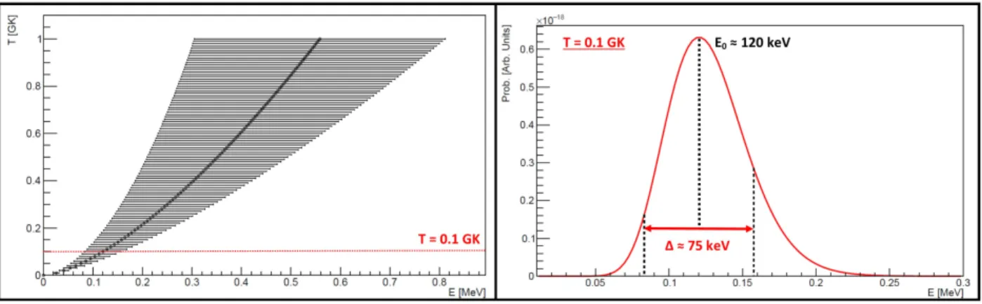
1.5 (Left) The stellar burning temperature is plotted as a function of Gamow peak energy centroid. The “error bars” associated with each of these Gamow energies represent the width of their corresponding Gamow peak. The red dotted line highlights the typical AGB hot-bottom burning temperature of 0.1 GK. (Right) The Gamow peak at 0.1 GK is illustrated. The corresponding energy centroid of this peak is given by Eq. 1.19 as E0≈120 keV with a width of∆≈75 keV, given by Eq. 1.20. . . 15
2.1 A diagram of the Laboratory for Experimental Nuclear Astrophysics is given above. The locations of the ECRIS and JN Van de Graaff accelerators (left), bending magnet for ion beam momentum analysis (center), and experimental target (right) are shown. Beam focusing and steering elements are labeled. . . 17
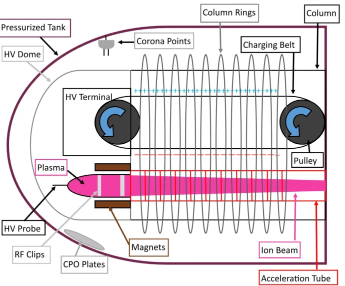
2.2 Schematic diagram of the ion source, high-voltage terminal and acceleration column of the Model JN 1-MeV accelerator. . . 18
2.3 A cut-away model of the ECR ion source plasma chamber with relevant components labeled. All displayed components are at chamber voltage, aside from the (green-yellow-green) ar-rangement of apertures at right. The green apertures sit at the potential of the high-voltage table, which is the ground reference for the chamber power supply, while the yellow aperture is biased slightly negative for electron suppression purposes. Microwaves are injected into the chamber from the left, an ECR discharge is struck within the aluminum chamber volume, and positive ions are extracted by the green aperture at right and accelerated to ground. . . 24
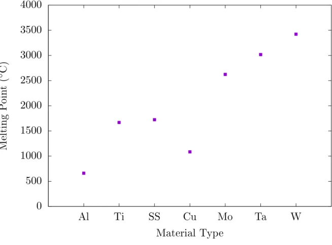
3.1 (Upper-left) A damaged 4 in to 2 in reduction adapter section of the beam line. This stainless steel section endured∼600 W of power for ∼30 s before the hole shown was created and a massive vacuum failure followed. (Upper-right) A titanium backing after receiving 800µA of DC proton beam at 200 keV for 6 C. Signs of localized melting are apparent on its surface. (Bottom) Beam collimation section of the LENA target station after sustaining∼100 W of poorly-focused beam for ∼ 1 hour. The left side of the copper tube was cooled to liquid nitrogen temperature, while the right side (just before the target) reached temperatures hot enough to melt silver solder. . . 30 3.2 Comparison of melting points of various metals used in beam line components and targets.
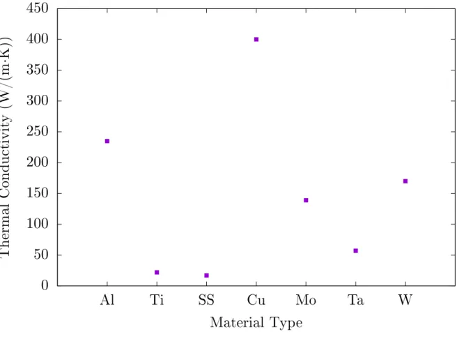
Note: “SS” denotes stainless steel. . . 31 3.3 Comparison of thermal conductivities of various metals used in beam line components and
targets. Note: “SS” denotes stainless steel. . . 32 3.4 An illustration of 1-Hz pulsed operation with a 10% duty cycle and an average target beam
current (ITgt) of 2 mA.. . . 33 3.5 Proof that plasma reignites to produce peak-pulsed beam current matching DC current, as
shown by digitally stored Faraday cup current signals with ECRIS pulsing for 100-ms on, 900-ms off. AC noise pickup is apparent in both signals, but largely hidden at the pulse peak by the DC trace. The DC beam current and energy were∼500µA and∼10 keV, respectively. The average pulsed current is thus∼50µA. . . 34 3.6 Data taken on the 151-keV resonance in the18O(p,γ)19F reaction using DC (red) and pulsed
(black) ECRIS beams for nearly the same integrated charge.. . . 35 4.1 Simulated beam profiles fromKassiopeiawith average radii illustrated by thick blue lines at:
a) our minimum operating energy (110 keV), b) 110 keV with a 5 kV retarding potential on the last conical electrode, and c) our maximum operating energy (230 keV). d) On-axis magnetic field orientations and magnitudes (sections A-D,∼15 mT; section E,∼4 mT), directions of Lorentz forces, and lateral beam displacements caused by our transverse magnetic suppression system. See text for further details.. . . 42 4.2 Cut-away view showing the ECR ion source and acceleration column assembly. . . 45 4.3 Construction details of the new acceleration column are given, with key parts that are discussed
in the text labeled as follows: a) Plasma chamber (PC); Plasma electrode (P); RingLess electrode (RL); Ceramic Insulator (CI); High-Voltage-Table electrode (HVT); Expansion Cone electrode (EC); conical Focus electrode (F); Shield Ring electrode (SR); Magnet Ring electrode (MR); magnet ring and Column electron Suppressor electrode (CS); Earth Ground (EG). b) Expanded view of the extraction region showing the beam Extraction electrode (E) and the Source Suppressor electrode (SS). Values of aperture diameters (d), axial thicknesses (t), and spacings (s) that define the beam are given in Table 4.1 or in the text. c) Expanded view of the junction between ceramic insulators and adjacent electrodes showing the dovetail O-ring groove. d), e) Detailed views of external and internal triple junctions, respectively, both electrostatically shielded inside an annular recess. . . 46 4.4 Oscilloscope voltage-versus-time traces of the beam scan (gold) and the downstream Faraday
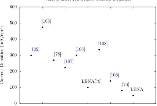
4.5 A comparison plot of experimentally measured plasma surface current densities of various high-intensity ECR ion sources. . . 54
4.6 Magnetic field intensity as a function of axial position within the ECR magnet. Measurements were collected with an F. W. Bell 7010 gaussmeter. The axial probe was inserted into the center hole of the ECR magnet plug target given in Fig. C.1. Each data point was collected by carefully moving the probe in 0.5-in increments down the bore of the magnet. The 875-G magnetic field intensity necessary for electron cyclotron resonance is denoted by the red dashed line to emphasize that this value is never attained on-axis within the ECR magnet. . 54
4.7 Magnetic field intensity (given according to the color gradient) as a function of axial and radial position within the ECR magnet. The wire-frame lines illustrate the inner diameter wall of the ECR magnet bore. Measurements were collected with an F. W. Bell 7010 gaussmeter. The axial probe was inserted into the radial holes (spaced 1-in apart) of the ECR magnet plug target given in Fig. C.1. Each data point was collected by carefully moving the probe in 0.5-in increments down the bore of the magnet. . . 55
5.1 Low-lying states of21Na, as given in Rolfset al. (1975) [2]. The energy level values, reaction Q-value, andJπ assignments are given in references [2, 10, 11]. . . . . 58
5.2 A detailed energy level diagram that conceptually illustrates how resonant proton capture into the 2425-keV state can occur via the high-energy tail of the Briet-Wigner cross section profile. This figure is given in reference [2]. . . 59
5.3 The astrophysical S-factor versus energy is given, as provided in reference [2]. The various resonant and direct capture components of the total S-factor are given and labeled accordingly. The dashed lines depict model predictions for various direct capture transitions, while the dashed-dot line represents the model prediction for capture into the high-energy tail of the subthreshold resonance at -7 keV. All of these models and their predictions are described in Ref. [2]. . . 60
5.4 Differential cross section versus beam energy measured at θγ = 90◦, as given in reference
[2]. Contributions from various resonances above the proton threshold are shown, along with theoretical predictions for low-energy contributions from the subthreshold resonance at -7 keV (solid line) and the direct capture transition to ground (dashed line). Note: the direct capture prediction represents an upper limit estimate for the cross section at low-energy. For more information, see this figure in reference [2].. . . 61
5.5 The fractional contribution of various resonances (denoted by their resonance energies) and DC processes (given as A-rates) to the total reaction rate versus burning temperature for the 20Ne(p,γ)21Na reaction, calculated using the
RatesMCsoftware package [12] and rate information fromSTARLIB[13]. The widths of each curve represent the present experimental uncertainty in the reaction rate contribution for nuclear process (resonant or DC). The lower dotted line represents the contribution from weak resonances (not explicitly labeled at the top) to the total reaction rate. . . 62
6.2 Outgassing by resistive heating with the evaporator at LENA. The bell-jar, with its protective containment mesh, is in place and a target backing is inserted within the high-vacuum envi-ronment. Contaminants within this target are being outgassed and pumped away. At right is the target box used to store all of the backings used in this experiment at rough vacuum when they are not in use. . . 68 6.3 Schematic of the NV-3206 Eaton ion implanter and its modified target station. . . 69 6.4 Electrical schematic of the NV-3206 Eaton ion implanter ion source as given in [15]. . . 70 6.5 Assembly drawing of the NV-3206 Eaton ion implanter ion source as given in [15]. . . 71 6.6 Tracks of 20-keV ions with differing masses through the double-focusing 90◦analyzing magnet
as given in [15]. . . 72 6.7 On-axis magnetic field magnitude versus coil current for a 2-in standard TUNL
electromag-netic steerer. Measurements taken with a FW Bell Model 7010 gaussmeter and hall probe.. . 76 6.8 Schematic of the ECRIS implantation beam line off of the 45◦-left port of the analyzing magnet. 77
7.1 Decay scheme for the Elab
r = 1169-keV resonance with energy level, branching ratio, and spin-parity information from Ref. [16]. . . 81 7.2 Target station and detector arrangement for the stoichiometric characterization of targets
use the 1169-keV resonance in the 20Ne(p,γ)21Na reaction at the end of the 52◦ beam line
in Target Room 01. Included in this image are the electrostatically-suppressed and liquid nitrogen-cooled cold trap, 55◦ lead shield, and germanium detector. See text for setup details. 82
7.3 Block diagram of the electronics setup used for signal processing and storage during the NRA measurements on the Elab
r = 1169 keV-resonance in20Ne(p,γ)21Na. See text for details. . . . 83 7.4 Detector arrangement for the target characterization measurements using NRA. The LENA
HPGe detector crystal (yellow) is oriented at 55◦ with respect to the beam axis and target
center. This figure was generated using the Fukui Renderer DAWN (Drawer for Academic WritiNgs) visualization application forGEANT4. . . 84 7.5 Energy level diagram illustrating the de-excitation of relevant nuclear states in60Ni following
theβ-decay of60Co. Energies and spin-parities of excited states in60Ni are given, along with theβ-decay reaction Q-value. . . 85 7.6 Residuals plot illustrating the method using to extrapolate60Co data to zero energy. See text
for details. . . 88 7.7 Measured and simulated full-energy absolute peak efficiencies for the 55◦ setup are given
7.8 Experimental yields versus beam energy using the 1169-keV resonance in20Ne(p,γ)21Na are given for each20Ne-implanted tantalum target backing in this NRA study. The stoichiometries of these targets were calculated from the integral of their measured yield over their energy widths.. . . 92 7.9 HPGe singles spectrum collected at 1172 keV on the Elab
r = 1169-keV resonance in the 20Ne(p,γ)21Na reaction, using neon-implanted tantalum target #4. This target is
∼ 8.50-keV-thick at Elab
r = 1169 keV. Labeled are the full-energy (FEP), single-escape (SEP), and double-escape (DEP) peaks associated with the primary and secondary decay branches from the reaction of interest (red), and peaks attributed to background sources (black). . . 93 8.1 a) The 52◦ scattering chamber with the position of the beam outlet, detector at 165◦, and
target ladder denoted. b) A 20Ne-implanted titanium target backing mounted to the target ladder via a clamp system for RBS analysis. A second target was mounted back-to-back with the one shown so that the target ladder could be rotated externally by 180◦ allowing for its
exposure to the4He2+ beam. . . . . 96 8.2 A block diagram illustrating the DAQ system employed for the RBS Run #1. Aside from the
detector and preamplifier used, this electronics setup was quite similar to the one presented in Section 7.2.1.. . . 98 8.3 An20Ne-implanted titanium target backing that exhibits faint, square RBS beam profiles on
center, and at 5- and 11-mm off-center to the right.. . . 99 8.4 A block diagram of the dedicated RBS DAQ system used in RBS Runs #2-5. See text for
details.. . . 100 8.5 An RBS scattering spectrum (illustrated inSIMNRA) of 2-MeV α-particles scattered from
a carbon foil with an evaporated layer of gold. The weak carbon peak is given at low energy (left) while the strong gold peak is at high energy (right). Au-C foil spectra like this were used for energy calibration purposes. . . 102 8.6 An RBS yield versus alpha particle scattering energy on 20Ne-implanted tantalum target
backing #3 is given above. Fitting regions are denoted, along with prominent spectral features that determine layer compositions. Fits to the data points are illustrated by the thin blue line.104 8.7 An RBS yield versus scattering energy on a20Ne-implanted titanium target backing is given
above. Fitting regions and prominent spectral features are denoted. . . 105 8.8 Expanded view of the front-edge region of bare (green) and20Ne-implanted tantalum targets
#3 (blue) and 4 (red). Scattering signal heights H1 and H2 denote the rough count levels in the bare and implanted front edges, respectively. . . 106 8.9 Expanded view of the front-edge region of bare (green) and20Ne-implanted titanium targets
#1 (red) and 2 (blue). Scattering signal heights H1 and H2 denote the rough count levels in the bare and implanted front edges, respectively. . . 106 8.10 Comparison plot of20Ne-implanted tantalum backing stoichiometries via RBS analyses.
Dag-ger superscript points denote stoichiometric values from yield curve measurements. (*) and (**) points were collected 5- and 11-mm off center, respectively.. . . 109 8.11 Comparison plot of 20Ne-implanted titanium backing stoichiometries via RBS analyses. (*)
8.12 A plot of the ratio f = ηi/ηf versus total accumulated beam charge is given. Here, ηi
andηf are the initial and final implanted target stoichiometries, given byη = NT a/N20N e. A degradation profile is provided by the three RBS measurements (purple points). A degradation correction factor was defined using a ratio of the total area (which assumes no degradation and is delineated by the black dotted line) to the cross hatched area (bounded by the degradation profile). . . 110
8.13 TRIM-2013simulations of 1169-keV protons propagated through a six-layer,20Ne-implanted tantalum target whose layer concentrations were given bySIMNRAfits to RBS measurements of Ne-Ta #3. (Left) Lateral beam profile within the target as a function of depth. (Right) Plots of beam energy loss to target atom ionization (black), effective stopping power (red), and lateral straggling (green) as functions of depth. . . 112
9.1 Decay scheme for the Elab
r = 384-keV resonance. Branching ratio and spin-parity information are given by Rolfset al.(1975) [2]. . . 114
9.2 ADAWNcut-away rendering of the LENAγγ-Coincidence Spectrometer and target station. Illustrated are the plastic scintillator cosmic-ray veto panels (blue), LENA HPGe detector (yellow, at center), NaI(Tl) annular array (green segments around HPGe), and lead (black). This represents the arrangement simulated inGEANT4and used in the peak efficiency anal-ysis given in Section 9.3.3. . . 116
9.3 A block diagram of the DAQ system for the LENAγγ-Coincidence Spectrometer. Note: black dots represent physical nodes; otherwise, wire crossings do not imply physical contact. See text for a detailed description of electronics logic. . . 118
9.4 A full-energy γ-ray peak efficiency curve for the LENA γγ-Coincidence Spectrometer. Red dots represent absolute efficiency measurements from60Co decay data, analyzed using the sum-peak method. Dark green dots are from scaled mono-energetic beam spot simulations from GEANT4. Black dots are from sum-corrected14N(p,γ)15O reaction data on the Elabr = 278-keV resonance. Blue dots are from sum-corrected 56Co decay data. See text for analysis details.. . . 120
9.5 On-resonance summed spectrum of all data collected at Elab
p = 392 keV on20Ne-implanted titanium targets #1, 2, and 4. Peaks associated with resonant capture in20Ne(p,γ)21Na are labeled in red, while prominent background peaks are labeled in black. . . 121
9.6 Enlarged portion of the spectrum given in Fig. 9.5 centered on the∼2466-keV primary line observed by Rolfs et al.(1975) [2]. Peaks associated with the Elab
r = 384-keV resonance are labeled in red, while background lines are labeled in black.. . . 122
9.7 All measured yield curves on the Elab
r = 384-keV resonance in 20Ne(p,γ)21Na that were col-lected on all four targets (panels a-d) used in this experiment. Fits to the data were carried out using Bayesian regression methods (see Appendix G). The integrated areas under these fitted curves were used to calculate individual resonance strengths for each target data set. See text for more analysis details.. . . 124
9.8 Comparison of Elab
9.9 Fractional contribution of direct (labeled as A-rates) and resonant (labeled by center-of-mass resonance energies) capture processes to the total reaction rate as a function of temperature for the 20Ne(p,γ)21Na reaction. The nuclear data input file used for these rate calculations was completely updated from that used to generate Fig. 5.5, and the new ECM
r = 366-keV resonance strength was included in these calculations. The burning region of interest for ONe classical novae is highlighted by the red vertical band. . . 129 10.1 Photographs of the primary components of the 55◦-90◦target arrangement. a) The angled e−
-suppressor tube, insulating ceramic section, and beam-collimation pipe are given. b) Angled beam pipe end with its elliptical flange is shown with the lead shield pulled back (at left). c) An overview showing the placement of each HPGe detector with respect to the target inside the lead shield (top-half is removed). . . 133 10.2 A block diagram of the 55◦-90◦ detection system electronics setup. Black dots denote wire
nodes; otherwise, wire crossings are not physical. See text for further signal processing details.136 10.3 ADAWNcut-away rendering of the 55◦-90◦detection system. This geometry was used in all
GEANT4simulations employed in the peak efficiency analysis given in Section 10.4. . . 138 10.4 A full-energy peak efficiency curve for the 55◦-90◦detection system. Absolute efficiency
mea-surements from60Co decay data, analyzed using the sum-peak method, are given in red (55◦)
and blue (90◦). Scaled mono-energetic beam spot simulations from
GEANT4 are given by red open (55◦) and blue closed (90◦) triangles. Sum-corrected 56Co decay data points are given in black (55◦) and yellow (90◦). Sum-corrected 14N(p,γ)15O reaction data points are given by the red (55◦) and blue (90◦) open circles. See text for analysis details. . . . 140
10.5 Summed Low gain HPGe singles spectrum (300-9000 keV) from the 55◦ detector, showing 30 C of20Ne(p,γ)21Na reaction data taken at a beam energy of Elab
p = 330 keV. Prominent environmental and beam-induced background signals are labeled in black. . . 141 10.6 SummedHighgain HPGe singles spectrum (200-3000 keV) from the 55◦detector, displaying
30 C of20Ne(p,γ)21Na reaction data taken at a beam energy of Elab
p = 330 keV. Environmental and beam-induced background signals are labeled in black. . . 142 10.7 Enlarged portion of the spectrum in Fig. 10.6 centered at ∼ 400 keV. Spectral regions of
interest for the 20Ne(p,γ)21Na reaction are labeled in red, while environmental and beam-induced background signals are labeled in black. . . 143 10.8 Enlarged portion of the spectrum in Fig. 10.6 centered at ∼ 2425 keV. Peaks associated
with the20Ne(p,γ)21Na reaction are labeled in red, while environmental and beam-induced background signals are labeled in black. . . 144 10.9 Same illustration given in Fig. 5.3 with the present measurements at Elab
p = 330 keV included. See text for details. . . 149 B.1 Geometric relation between bend radius and integrated field length as illustrated in Ref. [17]. 179 C.1 (Top) The various alignment targets used. Left to right: The ECR magnet plug target,
C.2 Brunson Model 76-RH190 transit scope used in precision alignment tasks for the ECRIS upgrade. See text for details on usage. . . 190 C.3 Target which fits into the flange connection at the ground end of the column. . . 191 C.4 Mylar cap target which fits over the source side of the fixed conical electrode. . . 192 C.5 A panoramic view of the ECRIS beam extraction system mounted on its axially adjustable
platform. The color-coded arrows point to horizontal (blue), vertical (yellow), pitch (yellow), and yaw (green) adjustments for aligning the extraction system apertures with the beam axis. All other cap-screws given are used for lock-down purposes. See text for details on these features and their usage. . . 193 C.6 (Left) The nosecone plug fiducial used to align the extraction aperture with the beam axis, as
seen through the transit scope. (Center) The ECRIS beam extraction system outside of the column−the red arrow emphasizes the insertion point of the peephole sight alignment target in the tail section. (Right) The peephole sight target as seen through the transit scope. See text for details on alignment methods. . . 194 C.7 (Left) The block-frame and pillar alignment assembly together. Notice the alignment pins
and roller-bearing set screws in the block-frame. There are top (as shown) and bottom (not shown) assemblies for the alignment of the copper plate. (Upper right) The block-frame with the pillar removed. (Lower right) The alignment pillar that mounts into a circular shoulder on the plasma electrode. . . 195 C.8 Example of the solenoid mylar targets. . . 197 D.1 An example 2D beam scan of ECRIS proton beam. The beam was momentum analyzed by a
magnetic focusing solenoid prior to this scan. . . 200 D.2 Oscilloscope traces of the beam scan (gold) and the downstream Faraday cup wire shadow
scan (blue), collected during the first 30-keV emittance test, are shown. . . 202 D.3 Beam scan data (blue), fitted with a Gaussian function (red), and residuals between the fit
and the data (black) for the first 30-keV emittance test are given above. . . 203 D.4 Shadow scan data (blue), fitted with a Gaussian function (red), and residuals between the fit
and the data (black) for the first 30-keV emittance test are given above. . . 204 D.5 Oscilloscope traces of the beam scan (gold) and the downstream Faraday cup wire shadow
scan (blue), collected during the second 30-keV emittance test, are shown. . . 205 D.6 Beam scan data (blue), fitted with a Gaussian function (red), and residuals between the fit
and the data (black) for the second 30-keV emittance test are given above. . . 206 D.7 Shadow scan data (blue), fitted with a Gaussian function (red), and residuals between the fit
and the data (black) for the second 30-keV emittance test are given above. . . 207 D.8 Oscilloscope traces of the beam scan (gold) and the downstream Faraday cup wire shadow
scan (blue), collected during the 100-keV emittance test, are shown. . . 208 D.9 Beam scan data (blue), fitted with a Gaussian function (red), and residuals between the fit
D.10 Shadow scan data (blue), fitted with a Gaussian function (red), and residuals between the fit and the data (black) for the 100-keV emittance test are given above. . . 210 E.1 Summed Low gain HPGe singles spectrum (300-9000 keV) from the 90◦ detector, showing
30 C of20Ne(p,γ)21Na reaction data taken at a beam energy of Elab
p = 330 keV. Prominent environmental and beam-induced background signals are labeled in black. . . 215 E.2 Summed High gain HPGe singles spectrum (300-9000 keV) from the 90◦ detector, showing
30 C of20Ne(p,γ)21Na reaction data taken at a beam energy of Elab
p = 330 keV. Prominent environmental and beam-induced background signals are labeled in black. . . 216 E.3 Enlarged portion of the spectrum in Fig. E.2 centered at ∼ 400 keV. Spectral regions of
interest for the 20Ne(p,γ)21Na reaction are labeled in red, while environmental and beam-induced background signals are labeled in black. . . 217 E.4 Enlarged portion of the spectrum in Fig. E.2 centered at ∼ 2425 keV. Spectral regions of
LIST OF ABBREVIATIONS
ADC Analog-to-digital converter
AGB Asymptotic giant branch
ANC Asymptotic normalization coefficient
BN Boron nitride
BNC Bayonet Neill-Concelman
BPM Beam profile monitor
CEA French Atomic Energy Commission
CFD Constant fraction discriminator
CMD Color-magnitude diagram
CNO Carbon nitrogen oxygen
CPO Capacitive pick-off
DAQ Data Acquisition
DFELL Duke Free Electron Laser Laboratory
DI Deionized
ECR Electron cyclotron resonance
ECRIS Electron cyclotron resonance ion source
EZH Electrostatic zonal harmonic
FC Faraday cup
FDU First dredge-up
FFA Fast filtering amplifier
FWHM Full-width at half-maximum
GC Globular cluster
GDG Gate-and-delay generator
GVM Generating voltmeter
HB Horizontal branch
HBB Hot bottom burning
HPGe High-purity germanium (HPGe)
HST Hubble Space Telescope
HV High-voltage
HVEC High Voltage Engineering Corporation
IMF Initial mass function
LED Leading-edge discriminator
LENA Laboratory for Experimental Nuclear Astrophysics
MCA Multichannel analyzer
Mg-Al Magnesium-aluminum
MS Main sequence
NaI(Tl) Thalium-doped sodium iodide
NdFeB Neodymium Iron Boron
NeNa Neon-sodium
NGC New General Catalog
NRA Nuclear reaction analysis
O-Na Oxygen-sodium
PN Planetary nebula
PVA Polyvinyl acetate
RBS Rutherford backscattering spectrometry
RF Radio-frequency
RGB Red giant branch
S-AGB Super-asymptotic giant branch
SBC Single board computer
SG Second generation SGB Subgiant branch
SDU Second dredge-up
TAC Time-to-amplitude converter
TDC Time-to-digital converter
TDU Third dredge-up
TFA Time filter amplifier
TO Main sequence turn-off point TPS Terminal potential stabilizer
TUNL Triangle Universities Nuclear Laboratory
UHR Upper hybrid resonance
CHAPTER 1: Introduction
Section 1.1: Nuclear Astrophysics: The Crossroads of The Large and Small
Stars are fueled by thermonuclear reactions within their cores [18, 19, 20, 21, 22]. Spectroscopic ob-servations of short-lived radionuclides in stellar atmospheres [23] and in the interstellar medium [24, 25] have proven that stars are nuclear furnaces, constantly forging and altering the chemical composition of the universe. Nuclear astrophysicists at facilities around the world seek to recreate these stellar environments terrestrially using nuclear fusion experiments focused on reactions that are astrophysically important. These reactions are typically those that are the most difficult for stars to complete at a given burning temperature. These bottleneck reactions determine the timescales for stellar evolution and nucleosynthesis. Rewards from these experiments are twofold: we learn about the extreme environments where stellar nucleosynthesis occurs and we can directly pinpoint where and how various nuclides are produced in the cosmos.
Researchers at the Laboratory for Experimental Nuclear Astrophysics (LENA) study astrophysically rel-evant thermonuclear reactions directly (i.e., via reactions involving the radiative capture of protons or4He nuclei). The specific science objective of LENA is the characterization of nuclear reaction rates that are central to the stellar life cycle. Knowledge of nuclear cross sections near or at stellar burning energies is pivotal for calculating the corresponding nuclear reaction rates. These cross sections can be vanishingly small because of dominance of Coulomb repulsion between reacting nuclei at such low energies (ranging from tens to hundreds of keV). Examples of recent experiments at LENA include studies of oxygen isotope production in late-stage stars and implications for stellar models using their observed abundances in presolar grains [26, 27]; precision low-energy measurements of the14N(p,γ)15O reaction and its importance for the timescale of the carbon-nitrogen-oxygen (CNO) burning cycle [28]; and measurements of the22Ne(p,γ)23Na reaction [29] relevant for the neon-sodium (NeNa) cycle and how this reaction could explain the observed oxygen-sodium (O-Na) abundance anticorrelation in globular cluster (GC) member stars (see Ref. [30] for a complete review of this field). The NeNa cycle is described schematically by [2,31],
In this thesis experiment, we investigate the20Ne(p,γ)21Na reaction (the first in this cycle) at low energies to further understand the evolution of globular cluster stars and their chemical abundances.
Experiments in nuclear astrophysics illuminate the past-lives of light-year-scale objects like globular clusters using femtometer scale processes. Hence, it is only fitting that their feasibility usually relies upon access to extraordinary instruments and expertise from several seemingly-separate fields. In order to carry out the project described in the following pages successfully (and the prior measurements listed above), we had to employ computational and experimental techniques from a multitude of differing fields including semiconductor fabrication, Bayesian statistics, nuclear spectroscopy, civil and mechanical engineering, high-voltage and pulsed power system operation, observational astronomy, ion source development, high-intensity beam acceleration and transport systems, and materials analysis. It is from this synthesis of laboratory skill and instrumentation that innovative instruments were conceived and built, new experimental methods were conceptualized and validated, and the frontier of nuclear astrophysics was tested and pushed.
The remainder of this chapter focuses on the fundamentals of stellar astrophysics of globular clusters and nuclear astrophysics experiments. In Chapter 2, the tools available at LENA are introduced and described. The development and operation of a pulsed electron cyclotron resonance ion source (ECRIS) are described in Chapter 3. Chapter4 documents a total upgrade of the acceleration column for the ECRIS at LENA. The current state of the low-energy data on the 20Ne(p,γ)21Na reaction is discussed and an experimental outline is given in Chapter 5. A complete account of target production methods via ion implantation is provided in Chapter6. Target characterization methods via nuclear reaction and Rutherford backscattering spectrometry analyses are given in Chapters7 and8. An improved resonance strength measurement of the Elab
r = 384 keV resonance is presented in Chapter 9. A new measurement of the 20Ne(p,γ)21Na reaction cross section at Elab
p = 330 keV is described in Chapter10. We close with a summary of experimental results, astrophysical implications, and a roadmap for future measurements in Chapter11.
Section 1.2: Not So Simple: Globular Clusters and the Oxygen-Sodium Anticorrelation
In the work below, we sought a deeper understanding of the evolution of globular clusters and chemical abundance anomalies exhibited by their member stars. Globular clusters are dense, spherical collections of stars that can be resolved into granular apparitions using a modest, backyard telescope. They have typical masses and radii of M∼104
−106solar masses (M) and R
within a given cluster are purely a result of its relative distribution of stars as a function of mass, known as its initial mass function (IMF). Typical cluster IMFs reveal that a minority of high-mass stars were formed, along with the majority population of lower-mass stars. The stellar lifetimes of these GC members can be estimated using scaling relations between stellar mass and luminosity, given by [32],
tlife∼ ML ∼M1−α, (1.2)
whereα∼1 for massive stars andα∼3 for intermediate-mass stars. Hence, even though all GC members are presumably of the same age, we find that the lower-mass component of the GC IMF has not yet pro-gressed to advanced evolutionary stages already completed by its higher-mass distribution.
1.2.1: Evolutionary Phases of Intermediate-mass GC Members
We can dive deeper into the evolution of GC members using a color-magnitude diagram (CMD). These di-agrams are variants of the temperature-luminosity plots made popular by Hertzsprung and Russell [33]. They provide evolutionary snapshots of the GC stars at progressively more advanced evolutionary stages (with necessarily higher masses), starting from the main sequence (MS) of the cluster. The evolutionary tracks of the stellar members inhabiting the prototypical GC M3 (Messier 3) are presented in Fig.1.1(originally given in Refs. [6] and [33]). Below, the major evolutionary stages and attributes of an intermediate-mass (∼5 solar masses) star are emphasized. The blue straggler (BS) group of stars, with their anomalous position above the main sequence in the CMD, are believed to be binary systems [33]. These objects will not be considered any further in this text.
We begin with GC members on the main sequence (MS). Stars composing this band are quiescently burning hydrogen within their cores (via the CNO cycle and proton-proton reaction chains) and experi-encing hydrostatic equilibrium (i.e., no expansion or contraction of their cores or envelopes). A typical intermediate-mass star has a MS lifetime of tM S ∼90 Myrs [33]. Stars that have left the main sequence via the turn-off (TO) point have exhausted their core hydrogen supply, while hydrogen shell burning continues just outside.
Figure 1.1: (Left) An image of the GC M3, courtesy of NASA/Karen Teuwen. (Right) A CMD of over 10,000 stellar members of M3, as given in Ref. [6]. Groups of stars are labeled according to their evolutionary type. See text and Ref. [6] for further details.
branch (RGB). Convection begins at this point in what is known as the first dredge-up (FDU) phase; this convection zone drives progressively deeper into the envelope as the star evolves up the RGB. Also, the first signs of processed nuclear material become observable in the stellar photospheres during the FDU phase.
An intermediate-mass star located at the RGB tip is just initiating core helium fusion under nonde-generate conditions [20, 33]. It will evolve over to the horizontal branch (HB) and maintain hydrostatic equilibrium via the triple-αprocess in its core and hydrogen burning in a surrounding shell. At this point, the energy output of the star steadily increases as the envelope and shell both contract. Progressing along the HB, core helium is exhausted as an inert carbon-oxygen (CO) core grows and a thick helium burning shell develops on top, with a subsequent hydrogen-burning shell above. As helium ashes from the shell above the CO core accumulate, the star enters another period of core contraction. Here, the helium shell narrows, energy production from it increases, and the hydrogen-burning shell above expands in response. Hence, this causes hydrogen-burning to intermittently cease in this region.
of the inactive hydrogen-burning shell, where a reservoir of helium resides. When the hydrogen-burning shell reactivates, nuclei in this so-called “hot bottom burning” (HBB) region [34] can experience advanced proton-capture reactions and then get convectively-cycled up to the surface for observation.
We continue our investigation up the AGB in Fig.1.1and encounter TP-AGB stars. These cluster mem-bers have electron-degenerate CO cores. As their cores receive more ashes from helium burning within the shell above, they continue to contract and the shell above expands. This temporarily extinguishes helium shell burning, the hydrogen shell above contracts and reignites, initiating HBB. The nuclear ash from this shell collects in the helium reservoir just below and the envelope expands again. The base of the helium reservoir eventually becomes electron-degenerate and periodic episodes of thermonuclear runaway occur after enough ash has accumulated. This causes the hydrogen shell to expand and extinguish− helium burning takes over again as the primary energy source. This process of alternating shell-burning episodes continues and, with each successively more explosive pulse cycle [35], mass is lost until the star enters its planetary nebula (PN) phase. These pulses also lead to the formation of a second convection zone in what is called the third dredge-up phase (TDU). This intershell (between the hydrogen and helium burning shells) convection commences in conjunction with the still-active envelope convection zone [33], and it cycles heavy nuclear products, from helium-burning deep within, upward, where subsequent HBB proton-captures can occur on them [31,34]. These HBB-processed nuclides are eventually cycled up to the surface via envelope convection. It is this combination of deep, convective cycles and violent mass loss episodes that likely allow TP-AGB stars to return processed nuclear material back to the interstellar medium [33, 30]. In closing, one should also notice that this processed material is retained within the gravitation potential well of a GC and not lost, as is the case for field stars that have entered their PN phase.
1.2.2: GCs as Cosmic Laboratories
can be determined using the distance modulus [33],
mGC−MGC0 = 5 log10
d
GC 10 pc
. (1.3)
Using fits to the MS in Fig. 1.1, the distances and luminosities of these cluster stars can be found (by a process known as main sequence fitting) and their masses can be determined via the empirical main sequence mass-luminosity scaling relation,
L∼Mβ, (1.4)
where β ∼ 3 for intermediate-mass stars [32]. Estimates from Eq.1.4 allow us to determine the masses of those stars located at the TO point in Fig.1.1, while Eq.1.2lets us reliably estimate their ages. Immediately, we can estimate the age of the cluster, and, hence, set a lower limit on the age of the galaxy and the universe [36,33,32,31,30].
In light of the results above, it is easy to be distracted by the use of GCs as only cosmological constraints, but there are other reasons why these objects are useful cosmic laboratories. Because they gravitationally retain newly-synthesized elements, they should provide us with the timescale on which heavy-element nu-cleosynthesis occurs. Also, they should be able to tell us about temporal and spatial differences in the evolution of the galactic chemical abundances [36]. However, these profound results only hold true if GC members are as homogeneous in origin and metallicity as was assumed at the beginning of this section. If multiple generations of stars exist within the cluster environment, each with differing helium abundances and metallicities, then the GC aging method via main sequence fitting is not as accurate as once thought and the use of these objects as galactic record-keepers becomes much more complicated.
1.2.3: Evidence and Formation Scenarios for Multiple Populations in GCs
Suspicions that there might be multiple stellar populations in GCs can be traced back to the RGB color investigations of Woolley [37] in the late 1960s, and various metallicity studies in the 1970s [38, 39]. Kraft (1979) was the first to point out several GC chemical abundance anomalies in a review of the existing literature, thereby giving this concept traction in subsequent studies [40]. Cotrell and Da Costa (1981) presented early observations of abundance enhancements of sodium and aluminum in members of the clusters 47 Tuc and NGC (New General Catalog) 6752 [41].
Figure 1.2: A CMD of the GCω Centauri as given by Bedin et al.(2004) [7]. These data were collected using the Wide Field Camera on theHST and it comprises the central part of the cluster. Clearly visible are multiple TO points and SGBs.
al.(2007) followed up withHST observations of NGC 2808 and found it harbored a triple-MS (see Fig.1.3)
−each MS band corresponded to a specific helium abundance value [8]. These results proved the existence of multiple GC stellar components, and strongly suggested they were associated with subsequent generations that had formed out of primordial GC stellar remnants.
Figure 1.3: A CMD of the GC NGC 2808, as given in Piottoet al.(2007) [8]. The data were collected using
HST observations and show a triple MS within this cluster. Each MS stellar band is discretely separated from another by its helium abundance, as illustrated in the inset image. See text and Ref. [8] for further details.
47,48,9,49,50,51,52,48,30] (O-Na) and magnesium and aluminum (Mg-Al) [53,54,55]. An example of
Figure 1.4: Sodium abundance versus oxygen abundance for stellar members of the globular cluster M13, as given in Johnson and Pilachowski (2012) [9]. The GC members are color-coded by their elemental abundances, with high oxygen and low sodium abundance deemed primordial (blue), while those rich in sodium and deficient in oxygen are called extreme (red) and are believed to have formed out of material that was chemically-enriched via nucleosynthesis. An intermediate (green) population exists between these two abundance groups. See text and Ref. [9] for further details.
our understanding of the GC O-Na anticorrelation origin using measurements and constraints from nuclear physics.
abundances, released them back into the cluster environment, and then second generation (SG) stars formed out of this enriched material. Furthermore, because the helium abundances of MS GC members exhibit a discrete structure (see MS band structure in Fig. 1.3), their star formation periods necessarily proceeded sequentially − i.e., each stellar generation was formed out of a single reservoir of material with a unique helium abundance [56]. Given this evidence, scenarios involving self-enrichment or accretion will not be considered as a viable model to explain the O-Na anticorrelation in GCs. In closing, it should also be noted that during a supernova event within the GC, most of the material is gravitationally unbound from the GC and lost. The small percentage (∼2%) of material that is retained does not exhibit the observed elemental abundances found in GCs [57].
Many different progenitor models have been hypothesized to explain the origin of these GC generations, including: massive stars [58, 59, 60], rapidly rotating stars [61, 62], binary systems [63,64], and AGB (and super-AGB) stars [65,66,35,67,68,69,70]. For various reasons (see discussions in Refs. [56] and [57]), all of these GC polluter models have flaws, but the AGB (and S-AGB) scenario presently appears most probable; therefore, it will be the only one considered in the following text.
1.2.4: The TP-AGB Scenario: Stellar Physics Constraints and Motivations for New Cross Section Measurements
The intermediate-mass TP-AGB star polluter model can satisfy the constraints from stellar physics that must be met by any candidate theory of GC evolution. The stellar wind velocities (∼ 10 km s−1) from these objects ensure that the nuclear-processed abundances will be gravitationally bound by the GC [57]. This model requires a FG stellar mass of MF G &3 M to reach typical HBB temperatures (T&30 MK) and initiate proton-captures at the bottom of the convective envelope [69]. By allowing these stars to only undergo a few TDU cycles, this mass cut-off limits their carbon abundances to match observations [33,56]. An upper mass limit on the FG stars of MF G .8 M is also imposed to avoid producing model stars that would result in core-collapse supernova events.
In order to produce GC abundance trends like those in Fig. 1.4, model AGB stars must experience a significant amount of HBB and sustain the NeNa and MgAl cycles for an adequate amount of time. These abundance production and destruction processes depend not only on HBB temperature, but also envelope convection efficiency, since a higher efficiency leads to a higher luminosity and, hence, a shorter AGB lifetime [35]. Therefore, the choice of convection model seems to dominate the physics uncertainties in the AGB polluter scenario [35]. However, well-known nuclear cross section data help inform this model selection process and their role in explaining abundance anomalies in GCs should not be underestimated.

![Figure 1.3: A CMD of the GC NGC 2808, as given in Piotto et al. (2007) [8]. The data were collected using HST observations and show a triple MS within this cluster](https://thumb-us.123doks.com/thumbv2/123dok_us/8328123.2208633/38.918.109.814.101.809/figure-given-piotto-collected-using-observations-triple-cluster.webp)


![Figure 5.1: Low-lying states of 21 Na, as given in Rolfs et al. (1975) [2]. The energy level values, reaction Q-value, and J π assignments are given in references [2, 10, 11].](https://thumb-us.123doks.com/thumbv2/123dok_us/8328123.2208633/88.918.264.667.107.687/figure-states-rolfs-energy-values-reaction-assignments-references.webp)
