Bounding the per protocol effect in randomized trials: an application to colorectal cancer screening

M E T H O D O L O G Y

Open Access

Bounding the per-protocol effect in

randomized trials: an application to

colorectal cancer screening

Sonja A. Swanson

, Øyvind Holme

, Magnus Løberg

, Mette Kalager

, Michael Bretthauer

, Geir Hoff

,

Eline Aas

and Miguel A. Hernán

Abstract

Background:The per-protocol effect is the effect that would have been observed in a randomized trial had everybody followed the protocol. Though obtaining a valid point estimate for the per-protocol effect requires assumptions that are unverifiable and often implausible, lower and upper bounds for the per-protocol effect may be estimated under more plausible assumptions. Strategies for obtaining bounds, known as“partial identification”methods, are especially promising in randomized trials.

Results:We estimated bounds for the per-protocol effect of colorectal cancer screening in the Norwegian Colorectal Cancer Prevention trial, a randomized trial of one-time sigmoidoscopy screening in 98,792 men and women aged 50–64 years. The screening was not available to the control arm, while approximately two thirds of individuals in the treatment arm attended the screening. Study outcomes included colorectal cancer incidence and mortality over 10 years of follow-up. Without any assumptions, the data alone provide little information about the size of the effect. Under the assumption that randomization had no effect on the outcome except through screening, a point estimate for the risk

under no screening and bounds for the risk under screening are achievable. Thus, the 10-year risk difference for colorectal cancer was estimated to be at least−0.6 % but less than 37.0 %. Bounds for the risk difference for colorectal cancer mortality (–0.2 to 37.4 %) and all-cause mortality (–5.1 to 32.6 %) had similar widths. These bounds appear helpful in quantifying the maximum possible effectiveness, but cannot rule out harm. By making further assumptions about the effect in the subpopulation who would not attend screening regardless of their randomization arm, narrower bounds can be achieved.

Conclusions:Bounding the per-protocol effect under several sets of assumptions illuminates our reliance on unverifiable assumptions, highlights the range of effect sizes we are most confident in, and can sometimes demonstrate whether to expect certain subpopulations to receive more benefit or harm than others.

Trial registration:Clinicaltrials.gov identifier NCT00119912 (registered 6 July 2005)

Keywords:Instrumental variable, Partial identification, Per-protocol effect, Colorectal cancer, Screening

Background

Most randomized trials report the intention-to-treat (ITT) effect as the primary, or only, measure of the comparative effect of the studied interventions. A focus on the ITT effect is attractive for several reasons [1, 2]. However, the ITT effect may not be the effect of interest

for patients and clinicians when there is a high rate of non-compliance or when the rate of non-compliance in the trial differs from that expected outside the trial set-ting. In such circumstances, the per-protocol effect – the effect that would have been observed had all trial participants followed the trial protocol – may be of greater interest [1, 2]. Unfortunately, when patient char-acteristics associated with non-compliance are also re-lated to patient outcomes, the naïve approach to estimating this effect in a “per-protocol analysis” re-stricted to those who follow the protocol in each arm of * Correspondence:[email protected]

1

Department of Epidemiology, Erasmus Medical Center, PO Box 2040, 3000 CA, Rotterdam, The Netherlands

2

Department of Epidemiology, Harvard TH Chan School of Public Health, Boston, MA, USA

Full list of author information is available at the end of the article

the trial will be biased. In these cases, identifying the per-protocol effect in a randomized trial requires strong assumptions (e.g., no unmeasured confounding) and methods that are commonly used in the analysis of non-randomized studies [2].

An alternative to estimating the per-protocol effect under these strong assumptions is to estimate lower and upper limits or“bounds”for the per-protocol effect under weaker, but perhaps more realistic, assumptions [3–8]. While effect bounding, known as“partial identification of the effect”, has been attempted in observational studies (particular in the social sciences), it is rarely implemented in randomized trials. This is surprising because partial identification methods can capitalize on assumptions that are expected to hold in many randomized trials.

Here we provide a guide to the use of partial identifica-tion methods in randomized trials with dichotomous out-comes and point interventions, i.e., interventions that are not sustained over time. As an example, we demonstrate the estimation of bounds for the per-protocol effect of colorectal cancer (CRC) screening on the 10-year risk of CRC incidence and death in the Norwegian Colorectal Cancer Prevention (NORCCAP) trial.

Methods

The NORCCAP trial

The design, procedures, and primary findings of the NORCCAP trial have been described elsewhere [9–11]. In brief, 98,792 residents of the City of Oslo and of Telemark County, Norway, who had no history of CRC and were aged 55–64 years in 1998 or 50–54 years in 2000 were ran-domly assigned to either treatment or control arms. Those selected for the treatment arm were invited to CRC screen-ing, including either a once-only flexible sigmoidoscopy or a combination of once-only flexible sigmoidoscopy plus an immunochemical fecal occult blood testing. Individuals assigned to the control arm were not offered any interven-tion. All participants who attended the screening provided written informed consent, and the study was approved by the Ethics Committee of South-East Norway and the Norwegian Data Inspectorate. Primary study endpoints

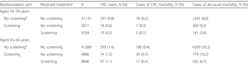
pre-specified in the study protocol were CRC incidence and mortality. Table 1 shows the 10-year risk of these outcomes [10] by age group, randomization arm, and screening intervention received. After standardization by age group, the ITT 10-year risk differences (95 % confi-dence interval) were −0.2 % (−0.4 %, −0.1 %) for CRC incidence, −0.1 % (−0.1 %, 0.0 %) for CRC mortality, and −0.2 % (−0.6 %, 0.2 %) for all-cause mortality.

Several features of this trial are relevant for our purposes. First, CRC screening was not available in the trial commu-nities for individuals not assigned to screening in the trial; thus, nobody in the control arm received it. Second, the treatment was a once-only screen (a point intervention); thus, compliance in the screening arm is all-or-nothing. Third, loss-to-follow-up was minimal; only 3 individuals were not followed until they experienced a study endpoint, emigration, or end of 10-year follow-up.

Overview of the analytic approach

The following sections describe the estimation of bounds for the per-protocol effect of point interventions on di-chotomous outcomes under increasingly stronger as-sumptions. We begin with no assumptions (i.e., the data alone), then assume the so-called “instrumental condi-tions” described below, and then combine additional as-sumptions with these instrumental conditions. Intuitively, the more assumptions we make, the narrower the bounds become, but of course this comes at a cost if our assump-tions are ill-placed. Table 2 summarizes the assumpassump-tions.

To compute the bounds in the NORCCAP trial, we first estimated bounds within age groups (50–54 years; 55–64 years) and then standardized these bounds. We begin by estimating the bounds in the older age group only so readers can check our calculations using the expressions provided in the text and the summary data in Table 1.

Results

Bounding the per-protocol effect under no assumptions

The per-protocol risk difference can theoretically range from−100 % (the treatment universally prevents the out-come) to 100 % (the treatment universally causes the

Table 110-year risk of colorectal cancer (CRC), CRC mortality, and all-cause mortality by randomization arm and treatment received

Randomization arm Received treatment N CRC cases,N(%) Cases of CRC mortality,N(%) Cases of all-cause mortality,N(%)

Aged 50–54 years

No screeninga No screening 37,131 297 (0.8) 78 (0.2) 2245 (6.0)

Screening No screening 2811 18 (0.6) 7 (0.3) 260 (9.2)

Screening 4109 19 (0.5) 5 (0.1) 141 (3.4)

Aged 55–64 years

No screeninga No screening 41,089 593 (1.4) 180 (0.4) 4209 (10.2)

Screening No screening 4806 74 (1.5) 34 (0.7) 779 (16.2)

Screening 8846 97 (1.1) 17 (0.2) 592 (6.7)

a

outcome). However, the study data–without any assump-tions–can be used to exclude parts of the theoretical range of the per-protocol effect. To see this, consider that, for every person in the study, we observe one of their two po-tential or counterfactual outcomes: e.g., for those who were screened, we see their outcome under screening, but do not know what would have happened to them had they not been screened (see illustration in Additional file 1: Table S1). We can compute bounds for the per-protocol effect by imputing the most extreme scenarios for the unobserved counterfactual outcomes–e.g., for the upper bound, im-agining that everybody who was screened would have ex-perienced the outcome had they not been screened, and that everybody who was not screened would have not experienced the outcome had they been screened. Thus, the per-protocol risk difference must lie within the bounds (using probability notation):

LB¼ðPr½Y¼1jX¼1−1ÞPr½X¼1 −Pr½Y¼1jX¼0Pr½X¼0 UB¼Pr½Y¼1jX¼1Pr½X¼1

þð1−Pr½Y¼1jX¼0ÞPr½X¼0;

whereXis an indicator of treatment,Yis an indicator of a dichotomous outcome of interest, and LB and UB

denote the lower and upper bounds, respectively. Ex-pressions for the risk under each level of treatment, the risk ratio, and a formal definition of the effect of interest are provided in the Additional file1.

The first block of Table 3 shows that these assumption-free bounds for the 10-year risk difference in the NORC-CAP trial are quite wide: e.g., from −10.0 to 90.0 % for CRC incidence. In fact, these bounds will always cover the null and necessarily have a width of 100 % for dichotom-ous outcomes. In order to obtain narrower bounds for the per-protocol effect we need to combine the data with assumptions.

Bounding the per-protocol effect under the instrumental conditions

The three instrumental conditions are often described as follows: (1) the randomization indicator (which we will denoteZ) is associated with receiving treatment X; (2) the randomization indicator Z causes the outcome

Yonly through treatmentX; and (3) the randomization indicator Z and the outcome Y share no causes [3]. The first condition, sometimes referred to as the “ rele-vance” condition, can be checked in the data: e.g., in the 55–64-year age group of the NORCCAP trial the risk difference:

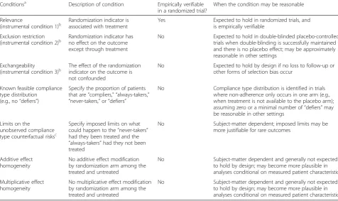
Table 2Description of analytic assumptions

Conditionsa Description of condition Empirically verifiable in a randomized trial?

When the condition may be reasonable

Relevance

(instrumental condition 1)b

Randomization indicator is associated with treatment

Yes Expected to hold in randomized trials, and is empirically verifiable

Exclusion restriction

(instrumental condition 2)b Randomization indicator has_{no effect on the outcome} except through treatment

No Expected to hold in double-blinded placebo-controlled trials when double-blinding is successfully maintained and there is no placebo effect; may be approximately reasonable in other settings

Exchangeability

(instrumental condition 3)b

The effect of the randomization indicator on the outcome is not confounded

No Expected to hold by design if no loss to follow-up or other forms of selection bias occur

Known feasible compliance type distribution

(e.g., no“defiers”)

Specify the proportion of patients that are“compliers,” “always-takers,”

“never-takers,”or“defiers”

No Compliance type distribution is identified in trials where non-adherence only occurs in one arm (e.g., when treatment is not available to the placebo arm); assuming zero or a minimal number of“defiers”may be reasonable in other settings

Limits on the

unobserved compliance type counterfactual risksc

Specify imposed limits on what could happen to the“never-takers” had they been treated and the

“always-takers”had they not been treated

No Subject-matter dependent; imposed limits may be more justifiable for rare outcomes

Additive effect homogeneity

No additive effect modification by randomization arm among the treated and untreated

No Subject-matter dependent and generally not expected to hold by design; may become more plausible in analyses conditional on measured patient characteristics

Multiplicative effect homogeneity

No multiplicative effect modification by randomization arm among the treated and untreated

No Subject-matter dependent and generally not expected to hold by design; may become more plausible in analyses conditional on measured patient characteristics

a

Bounds for the per-protocol effect presented in the current study rely on (1) no assumptions (data only); (2) the instrumental conditions; (3) the instrumental conditions, a feasible known distribution of compliance types, and imposed limits on unobserved compliance type counterfactual risks; (4) the instrumental conditions and additive effect homogeneity; and (5) the instrumental conditions and multiplicative effect homogeneity

b

Relevance, exclusion restriction, and exchangeability are jointly referred to as the instrumental conditions c

Pr½X¼1jZ¼1−Pr½X¼1jZ¼0 ¼0:65−0¼0:65:

Here, the F-statistic = 75626 andpvalue < 0.0001. The third “exchangeability” condition is expected by design in randomized trials. The second condition, known as the exclusion restriction, is expected to hold in double-blinded placebo-controlled randomized tri-als in which double-blinding is successfully maintained and there is no placebo effect, but may not hold in other trials, like ours. For example, the exclusion

restriction would be violated if the invitation letter alone prompted new awareness of CRC risk and risk factors, and subjects in the screening arm adopted preventive measures that they would not have adopted had they been in the control arm. Although we can-not prove conditions (2) and (3) hold in a given study, it is sometimes possible to find empirical evidence re-futing, i.e., falsifying, them [3].

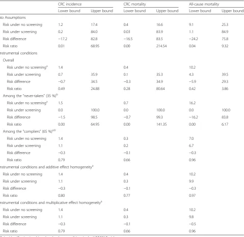
Under the instrumental conditions, we can compute the following bounds for the per-protocol risk difference: Table 3Lower and upper bounds for 10-year counterfactual risks and per-protocol effects among individuals 55–64 years old (units = cases/100 persons for risks and risk differences)

CRC incidence CRC mortality All-cause mortality

Lower bound Upper bound Lower bound Upper bound Lower bound Upper bound

No Assumptions

Risk under no screening 1.2 17.4 0.4 16.6 9.1 25.3

Risk under screening 0.2 84.0 0.03 83.9 1.1 84.9

Risk difference −17.2 82.8 −16.5 83.5 −24.2 75.8

Risk ratio 0.01 68.95 0.00 214.54 0.04 9.32

Instrumental conditions

Overall

Risk under no screeninga 1.4 0.4 10.2

Risk under screening 0.7 35.9 0.1 35.3 4.3 39.5

Risk difference −0.7 34.5 −0.3 34.9 −5.9 29.3

Risk ratio 0.49 24.88 0.28 80.64 0.42 3.86

Among the“never-takers”(35 %)b

Risk under no screeninga 1.5 0.7 16.2

Risk under screening 0.0 100.0 0.0 100.0 0.0 100.0

Risk difference −1.5 98.5 −0.7 99.3 −16.2 83.8

Risk ratio 0.00 64.95 0.00 141.35 0.00 6.17

Among the“compliers”(65 %)a,b

Risk under no screening 1.4 0.3 7.0

Risk under screening 1.1 0.2 6.7

Risk difference −0.3 −0.1 −0.3

Risk ratio 0.79 0.66 0.96

Instrumental conditions and additive effect homogeneitya

Risk under no screening 1.4 0.4 10.2

Risk under screening 1.1 0.3 9.9

Risk difference −0.3 −0.1 −0.3

Risk ratio 0.80 0.77 0.97

Instrumental conditions and multiplicative effect homogeneitya

Risk under no screening 1.4 0.4 10.2

Risk under screening 1.1 0.3 9.8

Risk difference −0.3 −0.1 −0.5

Risk ratio 0.79 0.66 0.96

a

Point identification is achieved under these conditions in the NORCCAP trial b

UB¼min

1−Pr½Y¼0;X¼1jZ¼1 þPr½Y¼1;X¼0jZ¼0;

1−Pr½Y¼0;X¼1jZ¼0 þPr½Y¼1;X¼0jZ¼1;

−Pr½Y¼0;X¼1jZ¼0 þPr½Y¼0;X¼1jZ¼1 þPr½Y¼0;X¼0jZ¼1 þPr½Y¼1;X¼1jZ¼0 þPr½Y¼0;X¼0jZ¼0; −Pr½Y¼0;X¼1jZ¼1 þPr½Y¼0;X¼1jZ¼0 þPr½Y¼0;X¼0jZ¼0 þPr½Y¼1;X¼1jZ¼1 þPr½Y¼0;X¼0jZ¼1;

Pr½Y¼1;X¼1jZ¼1 þPr½Y¼0;X¼0jZ¼1; Pr½Y¼1;X¼1jZ¼0 þPr½Y¼0;X¼0jZ¼0;

−Pr½Y¼1;X¼0jZ¼1 þPr½Y¼1;X¼1jZ¼1 þPr½Y¼0;X¼0jZ¼1 þPr½Y¼1;X¼1jZ¼0 þPr½Y¼1;X¼0jZ¼0; −Pr½Y¼1;X¼0jZ¼0 þPr½Y¼1;X¼1jZ¼0 þPr½Y¼0;X¼0jZ¼0 þPr½Y¼1;X¼1jZ¼1 þPr½Y¼1;X¼0jZ¼1

0 B B B B B B B B B B @ 1 C C C C C C C C C C A

Related bounds have also been proposed under dif-ferent interpretations of condition (3) [6, 8], but the bounds presented here make use of the strongest version of this condition expected to hold in ran-domized trials. See Richardson and Robins [12] for further discussion, including some intuition for these complicated expressions. See Additional file 1 for bounds for the (counterfactual) absolute risks under each treatment.

The second block of Table 3 shows that the bounds for the 10-year risk difference under the instrumental conditions are quite wide in the NORCCAP trial. For example, for CRC risk, the effect may fall anywhere between –0.7 % and 34.5 %. Interestingly, we can ob-tain a point estimate for the risk under no screening (for CRC risk: 1.4 %) but, because there is non-compliance in the screening arm, only bounds for the risk under screening (for CRC risk: 0.7 to 35.9 %). The wide bounds for the risk under screening drive the wide bounds for the risk difference.

Bounding the per-protocol effect within compliance types

Under the instrumental conditions, we can describe pa-tients in the study population as belonging to one of four mutually-exclusive “compliance types” or “ princi-pal strata”[13–15]:

(1)“Always-takers,”those who would have always been treated regardless of randomization

(2)“Never-takers,”those who would have always opted out of treatment regardless of randomization (3)“Compliers,”those who would have been treated

had they been randomized to receive treatment, and would not have been treated had they been randomized to the control arm

(4)“Defiers,”those who would not have been treated had they been randomized to receive treatment, but would have been treated had they been randomized to the control arm

For many trials, it may be reasonable to assume there are zero (or at least a small number of ) “defiers.” If we assume there are no “defiers” then we can identify the proportion of our study population who are in each of the other compliance types.

In the NORCCAP trial, there are no“always-takers”and no “defiers” because the screening was not available to those who were randomized to the control arm. There-fore, under exchangeability of the randomization arms, 35 % of trial participants are“never-takers”(estimated by Pr [X = 0|Z = 1]) and the other 65 % are “compliers”. For each person in the treatment arm we know whether she is a “complier” (if she did undergo screening) or a “ never-taker” (if she did not). In studies that have non-compliance in both randomization arms, we will not know with certainty any given subject’s compliance type.

Richardson and Robins [5] described bounds for the counterfactual risks and treatment effects within compli-ance types. In the special case when we (i) know there are only “compliers” and “never-takers” and (ii) have no empirical evidence against the instrumental conditions, then the effect within the “never-takers” is bounded as follows:

UB¼1−Pr½Y ¼1jX ¼0;Z¼1

LB¼−Pr½Y ¼1jX ¼0;Z¼1:

Meanwhile, the effect in the “compliers” is point-identified:

LB¼UB¼ Pr½Y ¼1jZ¼1−Pr½Y ¼1jZ¼0 Pr½X ¼1jZ¼1−Pr½X¼1jZ¼0 :

Beyond the special case where (i) is expected by de-sign, more general expressions have been described for an assumed distribution of compliance types [5]. Note that any assumed distribution needs to be feasible. For example, in studies like the NORCCAP trial with non-compliance in only one treatment arm, the only feasible LB¼ max

Pr½Y¼1;X¼1jZ¼1 þPr½Y¼0;X¼0jZ¼0−1; Pr½Y¼1;X¼1jZ¼0 þPr½Y¼0;X¼0jZ¼1−1;

Pr½Y¼1;X¼1jZ¼0−Pr½Y¼1;X¼1jZ¼1−Pr½Y¼1;X¼0jZ¼1−Pr½Y¼0;X¼1jZ¼0−Pr½Y¼1;X¼0jZ¼0;

Pr½Y¼1;X¼1jZ¼1−Pr½Y¼1;X¼1jZ¼0−Pr½Y¼1;X¼0jZ¼0−Pr½Y¼0;X¼1jZ¼1−Pr½Y¼1;X¼0jZ¼1; −Pr½Y¼0;X¼1jZ¼1−Pr½Y¼1;X¼0jZ¼1;

−Pr½Y¼0;X¼1jZ¼0−Pr½Y¼1;X¼0jZ¼0;

proportion of “defiers” is zero. In trials with non-compliance in both treatment arms, the data may be consistent with a range in the proportion of “defiers,” and investigators may consider computing bounds for the effects within compliance types under an assumed proportion of“defiers”within that range.

The second block of Table 3 further presents bounds for the counterfactual risks and per-protocol effect within the “compliers” and the “never-takers.” (In the NORCCAP trial, there is no evidence against the instru-mental conditions, so we can use the expressions de-scribed above.) For the “never-takers”, we can obtain a point estimate for the risks under no screening, but we have (by definition) no information on what would have happened to them had we forced them to follow the protocol in the screening arm and, therefore, been screened. Therefore, we can only achieve wide bounds for the per-protocol effect in the“never-takers” because we have limited information in the data on what would have happened to this subgroup had they followed the protocol. For the“compliers”, we can obtain a point esti-mate for the risks under screening and no screening, and, therefore, we can also obtain a point estimate for the per-protocol effect in the “compliers” [10], often re-ferred to as a“local”average treatment effect [15]. In the NORCCAP trial, the “compliers” are known to be those

who actually received the screening, and thus the effect in the“compliers”is the effect in the screened.

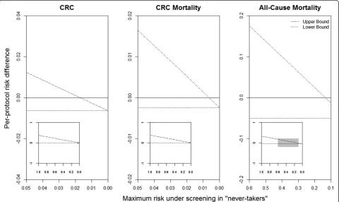
The bounds in the NORCCAP trial using the instru-mental conditions alone, described above, are a weighted average of the bounds in the “never-takers” and the point estimate in the“compliers”. In order to obtain nar-rower bounds for the per-protocol effect in the study population, we may combine the instrumental condi-tions with restriccondi-tions on the upper bound of the risk under screening in the“never-takers” (i.e., a counterfac-tual risk in 35 % of the study population for which we have no empirical information; Fig. 1) [5]. For example, we might assume that the risk under screening in the “never-takers” is actually not greater than their risk under no screening. Under this assumption, the resulting bounds do not include the null value: (−0.7 %, −0.2 %) for CRC risk, (−0.3 %, −0.1 %) for CRC mortality, and (−5.9 %, −0.2 %) for all-cause mortality. Though this as-sumption is plausible for CRC risk and mortality, it may not be for all-cause mortality, which could be more sus-ceptible to unintended consequences of screening. A less stringent restriction for all-cause mortality is that at most, say, 50 % of the “never-takers” would have died had they been screened. As seen in Fig. 1, this restriction (x-axis = 0.5) would imply bounds that include the pos-sibility of a null or positive risk difference. A sensitivity

analysis can be conducted under different hypothesized risks under screening in the “never-takers”, or the full range of possibilities could be presented as we do in the insets in Fig. 1. For trials with non-compliance in both treatment arms, similar sensitivity analyses could be conducted under hypothesized risks under no treatment in the“always-takers”.

Point identification of the per-protocol effect under the instrumental conditions plus homogeneity

The bounds can also be narrowed by combining the in-strumental conditions with assumptions that restrict ef-fect heterogeneity. In fact, when the instrumental conditions are combined with sufficiently strong homo-geneity assumptions, a point estimate of the per-protocol effect can be obtained [6, 7, 16]. Assuming (i) noadditiveeffect modification by the instrument among the treated and the untreated leads to what is often referred to as the standard instrumental variable (IV) estimator:

Pr½Y ¼1jZ¼1−Pr½Y ¼1jZ¼0 Pr½X ¼1jZ¼1−Pr½X ¼1jZ¼0:

Assuming (ii) no multiplicative effect modification by the instrument among the treated and the untreated leads to a different estimator:

Pr½Y¼1jX¼0Pr½X¼0ðexpð Þψ −1Þ

þ Pr½Y¼1jX¼1Pr½X¼1ð1−expð Þ−ψ Þ;

where

expð Þ ¼−ψ 1− Pr½Y ¼1jZ¼1−Pr½Y ¼1jZ¼0 Pr½Y ¼1jX¼1;Z¼1Pr½X¼1jZ¼1

−Pr½Y¼1jX¼1;Z¼0Pr½X¼1jZ¼0

:

In the NORCCAP trial, because we have only “ com-pliers” and “never-takers”, these assumptions could be restated as equal effects in the “compliers” and “ never-takers” on the (i) additive or (ii) multiplicative scale. Effect homogeneity assumptions may be implausible in many trials, particularly if there are interactions between patients’ treatment assignment and characteristics in informing treatment choice [16].

The third and fourth blocks of Table 3 shows the point estimates of the per-protocol risk difference under effect homogeneity on the additive and multiplicative scale, respectively. These assumptions will not hold in our study if, for example, family history of cancers modifies the effect of screening and patients in the screening arm with no family history of cancers may be more likely to forgo screening. The possibility for such modification is also apparent when examining the baseline risks across compliance types: the risk under no screening is lower in

the“compliers”than the“never-takers”which might indi-cate the magnitude of the effects in the “compliers” and “never-takers”could be very different. If family history and other relevant patient characteristics were mea-sured, it would be possible to relax the homogeneity as-sumptions (and instrumental conditions) to hold within levels of covariates and then present a point estimate of the per-protocol effect within levels of the covariates [6, 7, 16].

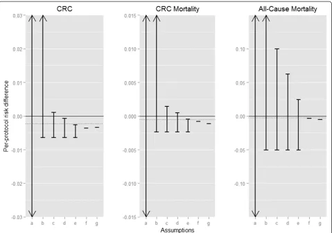
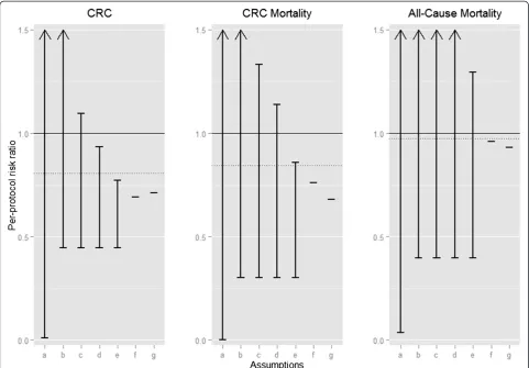
Bounds and point identification results for the per-protocol effect, aged 50–64 years

Thus far, we have considered bounding the counterfactual risks and the per-protocol effect among the 55–64-year age group. We repeated these computations for subjects aged 50–54 years (Additional file 1: Table S2). We then standardized by age group to obtain the estimates pre-sented in Additional file 1: Table S3; sex-stratified results are presented in Additional file 1: Table S4. The final age-standardized bounds for the per-protocol risk difference and risk ratio estimated under each set of assumptions are shown in Figs. 2 and 3. As demonstrated above with esti-mating the effect among the 55–64-year age group, the age-standardized bounds for the risk difference under the instrumental conditions are relatively wide (e.g., the risk difference for CRC incidence is between −0.6 % and 37.0 %), while narrower bounds or even point identification can be achieved by making additional assumptions about the possible magnitude and direc-tion of the effect in the “never-takers”.

Discussion

We have demonstrated how combining data with vari-ous sets of assumptions helps to bound the per-protocol effect of point interventions (i.e., interventions that are not sustained over time) in randomized trials with di-chotomous outcomes. In our application to a trial of CRC screening, we showed how bounds for both the per-protocol risk difference and risk ratio are achievable. Our application illustrates three key benefits of an ap-proach based on partial identification with progressively stronger assumptions.

First, this approach illuminates our reliance on unveri-fiable assumptions. In our trial, the wide bounds under no assumptions make clear that we cannot learn much at all about the effectiveness of screening without bring-ing in prior knowledge about the study design or our subject matter.

by 0.6 percentage points. This number provides a limit for how much our ITT effect estimate (−0.2 %) might underestimate the effectiveness under perfect adherence, and a boundary that could be helpful in evaluating the cost-effectiveness of screening or informing clinical or policy decisions. We know less about the upper bound (minimum effectiveness or even possible harm) of the screening program without making more debatable as-sumptions, but the type of analyses presented in Fig. 1 provides a template for discussing what level of assump-tions may be reasonable and how much differing opin-ions may lead to differing conclusopin-ions.

Third, this approach can demonstrate our confidence, or lack thereof, in the effect sizes for certain subpopula-tions [13–15]. In our trial, the estimates support the benefit of CRC screening for nearly two thirds of the study population (the “compliers”), and in this case we

subpopulation of “compliers” based on measured pre-randomization characteristics.

Investigators considering employing these methods in randomized trials with point interventions and dichotom-ous outcomes should consider how features of their par-ticular study design may affect which sets of assumptions we describe in Table 2 are reasonable. The instrumental conditions are expected to hold in placebo-controlled, double-blinded randomized trials of point interventions where there is no loss to follow-up, no placebo effect, and double-blinding is successfully maintained, but the in-strumental conditions are suspect in head-to-head randomized trials and whenever double-blinding is not successfully maintained or there is a possible pla-cebo effect. The homogeneity conditions, on the other hand, are not expected to hold based on any study design feature and thus should be weighed judiciously

when applied to the analysis of any randomized trial. A similar caveat applies to conditions about the dis-tribution of or effects within compliance types when there is non-compliance in both treatment arms [5].

methods to account for selection bias, e.g., inverse prob-ability weighting [19]. In trials that involve an interven-tion sustained over time, accounting for non-adherence can be more complicated as participants may discon-tinue the intervention at different times during follow-up and time-varying patient characteristics may inform and be affected by these decisions. More research is needed on how to generalize partial identification strat-egies to such settings, although the point-identification results can be expanded upon using structural nested models under related homogeneity and instrumental conditions [7, 20]. Finally, our example and discussion has focused on identification, but there is a growing body of literature on how to incorporate random variabil-ity [21]. Specifically, there has been recent development in methods for estimating confidence intervals around the bounds [22–26] as well as estimating confidence intervals for the partially identified treatment effect itself [27, 28]. Incorporating random variability into the presentation of partial identification results in randomized trials is critical; however, more research is needed as there is currently no consensus in the statistical literature on–or readily avail-able software for–the optimal approach.

The per-protocol effect is often of greater interest than, or complementary with, the ITT effect [1, 2]. In trials like the NORCCAP trial with essentially no loss to follow-up, we can easily compute an unbiased estimate for the ITT effect. However, the ITT effect quantifies the effect of assignment to treatment. From a patient’s perspective, deciding whether or not to take treatment requires knowledge about the effect of the treatment when received as intended rather than the effect of merely being assigned to treatment [1, 2]. Further, the ITT effect is study-specific because it depends on the magnitude and type of observed adherence to the intervention among study participants. That the per-protocol effect is independent of the observed adher-ence makes it interesting from a societal perspective too. For example, were the screening made available in the future to the Norwegian population, the actual adherence to the intervention could be different from that observed in the trial (not the least because the trial itself contributed to establish the efficacy of screening). As a result, the ITT effect from the trial would be outdated as a tool for decision-making, e.g., for cost-effectiveness analyses. On the other hand, un-biased estimates for the per-protocol effect, while po-tentially more relevant for decision making, are not achievable from the data alone: investigators need to combine the data with assumptions based on the study design and subject matter expertise. Historically, this has deterred many investigators from estimating the per-protocol effect as expert knowledge is, by def-inition, provisional and fallible.

Conclusion

As we have demonstrated using data from the NOR-CAPP trial, bounding the per-protocol effect under several sets of assumptions provides investigators with a middle ground between presenting a single value for the per-protocol effect based on sometimes heroic assump-tions versus avoiding estimating the per-protocol effect altogether. This middle ground shifts the scientific debate to what assumptions are most plausible and, therefore, to what range of effect sizes we are most confident in.

Additional file

Additional file 1:Norwegian Colorectal Cancer Prevention trial instrumental variable (NORCCAP IV) bounds trials submission supplement.Supplemental tables and an appendix describing the derivations for bounds not presented in the main text. (PDF 132 kb)

Abbreviations

CRC:colorectal cancer; ITT: intention-to-treat; IV: instrumental variable; NORCCAP trial: Norwegian Colorectal Cancer Prevention trial.

Competing interests

The authors report no competing interests.

Authors’contributions

SS, ØH, ML, MK, MB, GH, EA, and MH contributed to the conception of the current study. SS performed the data analyses and drafted the manuscript. ØH, ML, MK, MB, GH, EA, and MH contributed to the interpretation of the data and provided critical revisions. All authors read and approved the final manuscript.

Acknowledgments

This research was partly funded by National Institutes of Health grants R01 AI102634 and P01 CA134294.

Author details

1_{Department of Epidemiology, Erasmus Medical Center, PO Box 2040, 3000}

CA, Rotterdam, The Netherlands.2Department of Epidemiology, Harvard TH Chan School of Public Health, Boston, MA, USA.3_{Institute of Health and} Society, University of Oslo, Oslo, Norway.4Sørlandet Hospital Kristiansand, Kristiansand, Norway.5_{Telemark Hospital, Skien, Norway.}6_{Oslo University} Hospital, Oslo, Norway.7Cancer Registry of Norway, Oslo, Norway. 8_{Department of Biostatistics, Harvard TH Chan School of Public Health,}

Boston, MA, USA.9Harvard-MIT Division of Health Sciences and Technology, Boston, MA, USA.

Received: 27 April 2015 Accepted: 12 November 2015

References

1. Hernán MA, Hernandez-Diaz S, Robins JM. Randomized trials analyzed as observational studies. Ann Intern Med. 2013;159(8):560–2. doi:10.7326/0003-4819-159-8-201310150-00709.

2. Hernán MA, Hernandez-Diaz S. Beyond the intention-to-treat in comparative effectiveness research. Clin Trials (London, England). 2012;9(1):48–55. doi:10.1177/1740774511420743.

3. Balke A, Pearl J. Bounds on treatment effects for studies with imperfect compliance. J Am Stat Assoc. 1997;92(439):1171–6.

4. Hernan MA, Hernandez-Diaz S, Werler MM, Mitchell AA. Causal knowledge as a prerequisite for confounding evaluation: an application to birth defects epidemiology. Am J Epidemiol. 2002;155(2):176–84.

6. Robins JM. The analysis of randomized and nonrandomized AIDS treatment trials using a new approach to causal inference in longitudinal studies. In: Sechrest L, Freeman H, Mulley A, editors. Health service research methodology: a focus on AIDS. Washington, DC: US Public Health Service; 1989. p. 113–59.

7. Robins JM. Correcting for non-compliance in randomized trials using structural nested mean models. Commun Stat. 1994;23:2379–412. 8. Manski CF. Nonparametric bounds on treatment effects. Am Econ Rev.

1990;80(2):319-23

9. Bretthauer M, Gondal G, Larsen K, Carlsen E, Eide TJ, Grotmol T, et al. Design, organization and management of a controlled population screening study for detection of colorectal neoplasia: attendance rates in the NORCCAP study (Norwegian Colorectal Cancer Prevention). Scand J Gastroenterol. 2002;37(5):568–73.

10. Holme O, Loberg M, Kalager M, Bretthauer M, Hernán MA, Aas E et al. Colorectal cancer incidence and mortality after flexible sigmoidoscopy screening –First population-based randomized trial. JAMA. 2014;312(6):606-615 11. Hoff G, Grotmol T, Skovlund E, Bretthauer M. Norwegian Colorectal Cancer

Prevention Study G. Risk of colorectal cancer seven years after flexible sigmoidoscopy screening: randomised controlled trial. BMJ. 2009;338:b1846. doi:10.1136/bmj.b1846.

12. Richardson T, Robins JM. ACE bounds; SEMs with equilibrium conditions. Stat Sci. 2014;29(3):363-366.

13. Frangakis CE, Rubin DB. Principal stratification in causal inference. Biometrics. 2002;58(1):21–9.

14. VanderWeele TJ. Principal stratification–uses and limitations. Int J Biostat. 2011;7(1):1–14.

15. Angrist JD, Imbens GW, Rubin DB. Identification of causal effects using instrumental variables. J Am Stat Assoc. 1996;91(434):444–55.

16. Hernán MA, Robins JM. Instruments for causal inference: an epidemiologist’s dream? Epidemiology (Cambridge, Mass). 2006;17(4):360–72. doi:10.1097/01. ede.0000222409.00878.37.

17. Swanson SA, Hernán MA. Think globally, act globally: an epidemiologist’s perspective on instrumental variable estimation. Stat Sci. 2014;29(3):371–4. 18. Pearl J. Imperfect experiments: bounding effects and counterfactuals.

Causality. New York City: Cambridge University Press; 2009. p. 259–81. 19. Little RJ, D’Agostino R, Cohen ML, Dickersin K, Emerson SS, Farrar JT, et al. The

prevention and treatment of missing data in clinical trials. New Engl J Med. 2012;367(14):1355–60.

20. Robins JM. Structural nested failure time models. In: Anderson PK, Keiding N, editors. The encyclopedia of biostatistics. Chichester, UK: Wiley; 1998. p. 4372–89.

21. Tamer E. Partial identification in econometrics. Annu Rev Econ. 2010;2(1): 167–95.

22. Chernozhukov V, Hong H, Tamer E. Estimation and confidence regions for parameter sets in econometric models. Econometrica. 2007;75(5):1243–84. 23. Horowitz JL, Manski CF. Nonparametric analysis of randomized experiments

with missing covariate and outcome data. J Am Stat Assoc. 2000;95(449):77–84. 24. Manski CF, Sandefur GD, McLanahan S, Powers D. Alternative estimates of

the effect of family structure during adolescence on high school graduation. J Am Stat Assoc. 1992;87(417):25–37.

25. Ramsahai R, Lauritzen S. Likelihood analysis of the binary instrumental variable model. Biometrika. 2011;98(4):987-994.

26. Romano JP, Shaikh AM. Inference for identifiable parameters in partially identified econometric models. J Stat Plann Infer. 2008;138(9):2786–807. 27. Imbens GW, Manski CF. Confidence intervals for partially identified

parameters. Econometrica. 2004;72(6):1845-57.

28. Vansteelandt S, Goetghebeur E, Kenward MG, Molenberghs G. Ignorance and uncertainty regions as inferential tools in a sensitivity analysis. 2006; 16(3):953-979.

Submit your next manuscript to BioMed Central and take full advantage of:

• Convenient online submission

• Thorough peer review

• No space constraints or color figure charges

• Immediate publication on acceptance

• Inclusion in PubMed, CAS, Scopus and Google Scholar

• Research which is freely available for redistribution