Evolutionary Learning of Concepts

http://dx.doi.org/10.4236/jcc.2014.28008

Evolutionary Learning of Concepts

Rodrigo Morgon, Silvio do Lago Pereira

Department of Information Technology, FATEC-SP/CEETEPS, São Paulo, Brazil Email: [email protected], [email protected]

Received 24 April 2014; revised 20 May 2014; accepted 19 June 2014

Copyright © 2014 by authors and Scientific Research Publishing Inc.

This work is licensed under the Creative Commons Attribution International License (CC BY). http://creativecommons.org/licenses/by/4.0/

Abstract

Concept learning is a kind of classification task that has interesting practical applications in sev-eral areas. In this paper, a new evolutionary concept learning algorithm is proposed and a cor-responding learning system, called ECL (Evolutionary Concept Learner), is implemented. This sys-tem is compared to three traditional learning syssys-tems: MLP (Multilayer Perceptron), ID3 (Iterative Dichotomiser) and NB (Naïve Bayes). The comparison takes into account target concepts of varying complexities (e.g., with interacting attributes) and different qualities of training sets (e.g., with imbalanced classes and noisy class labels). The comparison results show that, although no single system is the best in all situations, the proposed system ECL has a very good overall performance.

Keywords

Evolutionary Algorithms, Machine Learning, Classification, Interaction, Imbalance, Noise

1. Introduction

The ability to learn through experience is crucial for intelligent behavior. In fact, machine learning [1] is an im-portant research area in artificial intelligence that studies learning as the result of computational processes. The main goal of machine learning is to design algorithms that can learn, or rather, that can automatically improve their performance on certain tasks as result of experience. There are a wide variety of tasks and corresponding methods studied in machine learning (e.g., classification, clustering and association). In this paper, the focus is on concept learning, a kind of classification task that has interesting practical applications in several areas [2].

An algorithm that learns from examples must find a hypothesis, in the space of all possible hypotheses, which best characterizes objects belonging to a target concept. The size and complexity of this search space depend on how the hypotheses are represented by the algorithm (representational bias). Indeed, the representational bias can make some kinds of concepts easier to learn and, simultaneously, it can make some others harder. Further-more, due to the size and complexity of the search space, learning algorithms often make use of some heuristics that can guide them towards simpler and more general concepts (searching bias). However, even employing good and admissible heuristics, there is no guarantee of a good performance for all kinds of concepts [1].

Besides the representational and searching biases, there are many other factors that can affect the performance of a learning algorithm, for instance: imbalance, characterized by training sets that have too few examples in one class and too many examples in the other one [4]; interaction, characterized by target concepts that are defined in terms of independent attributes with synergetic effects [5]; and noise, characterized by training sets that have some incorrectly labeled examples [6]. Clearly, all these factors depend uniquely on the specific training set that is given as input to a learning algorithm. Thus, in order to enhance its robustness and its overall performance, a learning algorithm must be able to adapt itself for each possible quality of input. In fact, adaptation seems to be an important element for a good overall performance in concept learning.

Evolutionary algorithms [7] are known to be a powerful adaptive search method for large and complex spaces and, indeed, there are several works in the literature that explore the use of such kind of algorithm in the context of classification [8]. In this setting, the evolutionary algorithm evolves a population of individuals representing possible hypotheses. At each generation, the fitness of each individual (e.g., the accuracy of the corresponding hypothesis with respect to the training set) is computed and some of the best individuals are selected to give birth to new individuals that will possibly compose the next generation. This process is repeated until some ter-minal condition is satisfied (e.g., a maximum number of generations is achieved). At the end, the best individual in the population is returned as the algorithm’s output.

In this paper, a new evolutionary concept learning algorithm is proposed and a corresponding learning system, called ECL (Evolutionary Concept Learner), is implemented. This system is compared to three traditional learning systems [1]: MLP (Multilayer Perceptron), ID3 (Iterative Dichotomiser) and NB (Naïve Bayes). The comparison takes into account target concepts of varying complexities (e.g., defined in terms of interacting attributes) and different qualities of training sets (e.g., with imbalanced classes and noisy class labels). The comparison results show that, although no single system is the best in all situations, the proposed system ECL has a very good overall performance.

The rest of this paper is organized as follows: Section 2 introduces the fundamentals of concept learning; Sec-tion 3 presents the proposed evoluSec-tionary concept learning algorithm and describes details of the ECL’s imple-mentation; Section 4 describes the datasets used in the comparison of the four learning systems, and presents the empirical comparison results; finally, Section 5 presents the conclusions of this paper.

2. Concept Learning

This section presents the fundamentals of concept learning, based on which the system ECL was implemented.

2.1. Objects and Concepts

A simple way of describing objects is by using attribute tuples. An attribute is a variable that can be qualitative (nominal or categorical) or quantitative (discrete or continuous). In this work, only nominal attributes are consi-dered. The set of all possible objects, or instances of an attribute tuple, is called instance space or universe. For example, consider a simplified version of the Monks problem [9], in which the objects are robots described by attribute tuples of the form (color, smiling, holding), where the three attributes have the following domain: color

∈ {red, green, blue, gray}, smiling ∈ {yes, no}, holding ∈ {sword, balloon, flag}. Clearly, the set of all poss-ible robots has exactly 4 × 2 × 3 = 24 objects; that is, the size of the instance space is 24.

A concept can be formally defined as a function from the instance space to the binary set

{ }

+ −, or, rather, to the Boolean set {true, false}. In this sense, a concept is a logical predicate that defines a set of objects satisfying a precise condition. For example, the concept of a friendly robot can be described by the Boolean expression (smiling = yes) and not (holding = sword). According to this concept description, the set of all friendly robots, a subset of the instance space, has only 8 objects.

robots (i.e., a true proposition about friendly robots). Let F0 be the set of all features derived from the attributes,

and their corresponding values, which are used to describe objects in a specific context. The set of all Boolean expressions that can be formed with features drawn from F0 is called the hypothesis space. It is worth to notice

that a Boolean function can be represented by various syntactically distinct Boolean expressions, but each Boo-lean expression can represent only one BooBoo-lean function. For example, in the Monks problem context, not (holding = sword) and (holding = balloon) or (holding = flag) are distinct expressions representing the same function. In fact, there are 22n Boolean functions over n features; however, there are infinitely many syntacti-cally distinct Boolean expressions which can be formed with n features. Therefore, the size of the hypothesis space for arbitrary Boolean expressions is infinite.

2.2. Examples and Datasets

Let  be a concept in a universe  . An object x∈ is a positive example of  if x∈; otherwise, x is a negative example of . For example, the object (red, yes, flag)is a positive example of friendly robot, while the object (blue, yes, sword) is a negative one. A labeled example is a pair

( )

x y, , where x is an object and

{ }

,

y∈ + − is a class label. For example, both the pairs ((red, yes, flag), +)and ((blue, yes, sword), −) are cor-rectly labeled examples of the concept “friendly robot”.

A set of labeled examples of an unknown target concept  is called a dataset. Frequently, a dataset is di-vided into two parts called training set and validation set. The training set is used by the learning system to find the hypothesis  that best agrees with  in predicting the class of unseen objects of  . The validation set is used to evaluate the performance of the hypothesis found by the system.

There are different qualities of datasets. An imbalanced dataset is a dataset that has too few examples in one class and too many examples in the other one [4]. A noisy dataset is a dataset containing incorrectly labeled examples. The quality of a dataset can negatively affect the quality of the hypothesis found by the learning sys-tem [6].

2.3. Hypothesis Evaluation

The hypothesis returned as output by a learning system is a function  that maps objects of a specific universe  to their corresponding class labels. Indeed, it is expected that such hypothesis can assign unseen objects to their corresponding class labels with high performance.

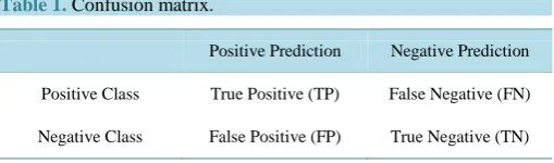
The most common performance metrics used to hypothesis evaluation are based on the analysis of a confu-sion matrix, as shown in Table 1. Such matrix is created by comparing 

( )

x to y, for each example

( )

x y, in the validation set. When 

( )

x = y, we have a true positive (if y= +) or a true negative (if y= −). Con-versely, when 

( )

x ≠ y, we have a false positive (if y= −) or a false negative (if y= +).

A number of performance metrics widely used to hypothesis evaluation can be extracted from a confusion matrix [10]. The accuracy, defined as

(

TP TN+

) (

TP+FP+FN+TN

)

, is the percentage of objects correctly classified by a hypothesis. The True Positive Rate (TPR), defined as TP TP

(

+FN

)

, is the percentage of ob-jects correctly classified as positive examples. The True Negative Rate (TNR), defined as TN

(

FP TN+

)

, is the percentage of objects correctly classified as negative examples.

[image:3.595.171.426.642.717.2]

It is worth to notice that accuracy is not a good metric to be used with imbalanced datasets, since it favors hypotheses which are strongly biased to the majority class. For example, consider a hypothesis  that classi-fies all objects of its universe as negative examples. Thus, if an imbalanced dataset contains only 1% of positive examples (minority class), the hypothesis  has an accuracy of 99%. In fact, a better performance metric to deal with imbalanced datasets is the g-measure, defined as the geometric mean of TPR and TNR. Clearly, using this metric, we can favor hypotheses with high percentages of correctly classified objects, in both classes.

Table 1. Confusion matrix.

Positive Prediction Negative Prediction

Positive Class True Positive (TP) False Negative (FN)

3. The Evolutionary Approach

The evolutionary approach [11] is based on stochastic search algorithms which are inspired in the Darwinian theory of evolution. Several different techniques are grouped under the generic denomination of evolutionary algorithm [12]. All such techniques share three main characteristics: the use of a population of individuals representing candidate solutions; the use of genetic operators to generate new individuals in the population; the use of a fitness measure to select individuals of the population which must survive from one generation to the next one.

The particular algorithm proposed in this work borrows ideas from different canonical evolutionary algo-rithms. From genetic programming [13], it borrows the idea of representing the individuals in the population by trees; from evolutionary programming [14], it borrows the idea of applying only mutations to generate new in-dividuals in the population; and, from evolution strategy [15], it borrows the µ µ+ selection scheme to evolve the population from one generation to another. These ideas, based on which the system ECL (Evolutionary Concept Learner) was implemented, are discussed in more details in the next subsections.

3.1. Tree Generation

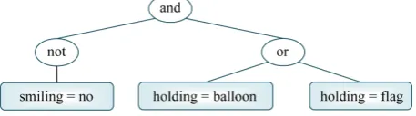
A Boolean expression can be easily represented by a tree whose internal nodes are labeled by logical operators and whose leaf nodes are labeled by features. For example, Figure 1 shows the tree representation of the ex-pression not (smiling = no) and ((holding = balloon) or (holding = flag)). The tree representation can simplify the implementation of the various operations over Boolean expressions (e.g., creation, mutation and evaluation) that must be performed by our evolutionary algorithm.

In genetic programming [13], there are two basic methods of generating random trees to form the initial pop-ulation: the full method and the grow method. The full method generates complete trees in which all leaf nodes are at the same level. On the other hand, the grow method generates trees of various shapes. Although easy to implement, these methods cannot guarantee a uniform distribution of the generated trees, since they choose fea-tures and operators to label the tree nodes with equal probabilities. Thus, for example, when there are signifi-cantly more features than operators, the grow method almost always generates very short trees. Conversely, when there are significantly less features than operators, the grow method behaves almost like the full method. To overcome this limitation, a different approach is adopted in our proposed algorithm.

Our algorithm’s input is given in the standard Attribute-Relation File Format (ARFF) [16], where each attribute is defined by its name and its domain. Let a be an attribute with domain

{

ν

₁,,

ν

_k

}

. The set of all features derived from a is

{

a=

ν

₁,,a=

ν

_k

}

. For example, the set of features derived from the attribute smil-ing, with domain {yes, no}, is {smiling = yes, smiling = no}. Let F0 be the set of all features derived from all the

attributes, and their corresponding domains, defined in the input file (notice that the elements of F0 can be

viewed as a nullary operators, i.e., operators that have no operands). Let F1 be the set of unary operators (e.g.,

not) and F2 be the set of binary operators (e.g., and, or). Then, the random trees generated must have their leaf

nodes labeled by elements of F0 and their internal nodes labeled by elements of F1∪F2.

In our approach, the distribution of random trees is based on an upper bound for the number of trees, with height at most h, that can be composed by nullary, unary and binary operators. This upper bound, T_h, is induc-tively defined as follows: If h=1, the tree’s root label must be chosen in the set F₀; thus, T₀= F₀ . On the other hand, if h>1, each tree rooted by a nullary operator is a tree of height at most h; each tree of height

1

h− , extended with a root labeled by a unary operator, is a tree of height at most h; and each pair of trees of height h−1, combined by a root labeled by a binary operator, is a tree of height at most h; thus

2

0 1 1 2 1

h h h

[image:4.595.200.429.642.706.2]

T = F + F T⋅ ₋ + F ⋅T₋ . Therefore, uniform distribution of the random trees in our implementation is guaranteed by choosing a nullary, a unary and a binary operator to label the root of a tree with probabilities

0 h

F T ,

(

F T₁ ⋅ _h−₁

)

T_h , and

(

F2 ⋅Th2−1

)

Th, respectively, and by recursively creating its subtrees.

3.2. Tree Mutation

Once created, a tree can be modified by a mutation function. This function randomly selects one of a number of basic modifications that can be applied on a tree, applies the modification and returns the resulting tree.

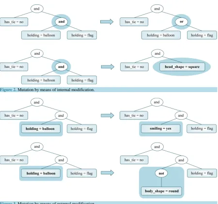
When an internal modification is applied, an internal node of the tree is randomly selected and its label is randomly replaced by other label of the same arity (preserving the tree height) or the subtree rooted by it is re-placed by a random tree of height at most 2 (possibly decreasing the tree height), as depicted in Figure 2.

When an external modification is applied, a leaf node of the tree is randomly selected and its label is random-ly replaced by another nullary operator (preserving the tree height) or the subtree rooted by it is replaced by a random tree of height at most 2 (possibly increasing the tree height), as depicted in Figure 3.

In our algorithm, mutation is the unique genetic operation applied to evolve individuals in a population.

3.3. Tree Evaluation

As before mentioned, each tree represents a possible hypothesis about the unknown target concept defined by a specific training set. Thus, the quality of a tree depends on its evaluation on that training set.

[image:5.595.89.540.294.715.2]

Figure 2. Mutation by means of internal modification.

In our algorithm, the tree evaluation relies on lambda functions of the form

(

λ

a₁,,a_k :

β

)

, where β is a Boolean expression over features derived from the attributes a₁,,ak. Given a tree t, a corresponding lambda function, , can be easily obtained. Moreover, since each example in a training set is a pair

( )

x y, , where x is an object in the instance space defined by the attributes a₁,,ak, the class label assigned to x by a tree t can be easily determined by evaluating _t

( )

x . Thus, a confusion matrix for t can be obtained simply by evaluating

( )

t x

 , for each object in the training set (see Subsection 2.3). From this matrix, some performance metrics for t can be extracted, for example, its accuracy and its g-measure.

3.4. Tree Selection

In genetic programming, the most widely used method to generate the initial population is known as ramped half-and-half [13]. This method results from the combination of two simpler methods, called full method and grow method. As mentioned in Subsection 3.1, these methods cannot guarantee a uniform distribution of the trees in the initial population. Thus, to ensure this property, our algorithm employs a uniform random tree gene-rating function to create the initial population. Furthermore, to ensure that all trees in the population are distinct from each other, the algorithm uses a hash table to store the population. In fact, in this hash table, each tree t is a key to which are associated its g-measure g t

( )

, i.e., the performance measure of t in the training set, and its size s t

( )

, i.e., the number of nodes in t. This technique avoids reprocessing of identical trees, which is a waste of computational resources, and also increases diversity, which is usually beneficial.

At each generation, the algorithm transforms the current population into a new population, by using the µ µ+ selection scheme [15]. First, each one of the µ trees in the current population produces a distinct mutant offspring that is included in the population (i.e., a new entry with a tree, its g-measure and its size is created in the hash table). Then, from this resulting population containing µ µ+ distinct trees, only the µ trees with highest fitness are selected to survive in the next generation. This selection scheme is highly elitist and ensures that, all along the evolutionary process, the average fitness of the population never decreases.

The fitness of a tree is a value highly dependent of its g-measure. Therefore, trees with higher g-measures must also have higher fitness. Moreover, according to the principle of parsimony, known as Occam’s razor [13], the best hypothesis is always the simpler one. Then, to avoid overfitted hypotheses (i.e., hypotheses with high performances in the training set, but poor performances in the validation set), simpler and more general hypo-theses must be preferred. Therefore, trees with shorter sizes must also have higher fitness. Thus, the goal of the evolutionary process is to maximize g-measures and, as much as possible, to minimize sizes.

Let

γ

and σ be, respectively, the g-measure and the size of the best tree in the parent population. The weight of an offspring tree t relatively to the best parent tree is w t

(

, ,γ σ

)

=

(

g t

( )

−γ

)

+

(

σ−s t

( )

)

⋅10−6+π where π is a preference value, as defined in Table 2. The fitness of a tree t is g t

( ) (

⋅w t, ,

γ σ

)

. When the conjoined population of parents and offspring is sorted in decreasing order of fitness, the µ trees with higher g-measures and shorter sizes are positioned in the first half of the resulting sequence. Thus, by taking the first half of this sequence, we have the fittest trees that must survive in the next generation.

3.5. The System Implemented

[image:6.595.168.425.628.717.2]

Based on the ideas presented hitherto, an evolutionary concept learning system, called ECL (Evolutionary Con-cept Learner), was implemented in Python [17]. This language was chosen due to its facilities to deal with trees, hash tables and lambda functions. The system is composed by two functions: the first evolves a population of hypotheses and, at the end, returns the best hypothesis in the population (w.r.t. the training set); and the second evaluates this best hypothesis (w.r.t. the validation set) and reports some corresponding performance statistics.

Table 2. Preference values.

( )

s t <σ s t( )=σ s t( )>σ

( )

g t >γ +0.004 +0.003 +0.002

( )

g t =γ +0.001 0 −0.001

( )

4. Empirical Results

The experiments described in this section compare ECL to three other traditional learner systems [1] which are implemented in Weka (Waikato Environment for Knowledge Analysis) [16]: MLP (Multilayer Perceptron), ID3 (Iterative Dichotomiser), and NB (Naïve Bayes). The aim of these experiments is twofold: first, to verify how ECL behaves in presence of interactions, imbalance and noise; and, second, to verify whether its performance in real word applications can be comparable to that of standard methods in machine learning. To achieve this aim, a broad empirical evaluation, using 15 artificial datasets and 14 natural datasets, was performed.

The artificial datasets were specially designed to provide some insights into the ability of the system ECL to cope with characteristics that is commonly found in real situations, and that can negatively affect the perfor-mance of a learning system. To generate these datasets, we have implemented a program that receives as input the following parameters: the number of Boolean attributes describing the instance space, the Boolean expres-sion describing the concept whose examples must be generated, the training set size, the validation set size, and the percentage of noise in the training set. As output, this program generates two ARFF files, one of them representing the training set and the other representing the corresponding validation set.

In order to evaluate the performance of ECL in real situations, we have also performed experiments with nat-ural datasets (i.e., datasets whose examples are derived from real world applications). These datasets were se-lected from two well known machine learning repositories (KEEL [18] and UCI [19]). To select these datasets, we have taken into account the attribute types used to describe their examples and also the number of classes. Only datasets with nominal attributes were selected. Besides that, for datasets with more than two classes, we have randomly chosen a class as positive class and collapsed the remaining classes as the negative class.

In all experiments, the same datasets were used as input for all the compared systems. Moreover, all ECL’s results reported were obtained with a population of 25 trees and 20 runs, each one with at most 5000 generations, for each dataset.

In the next sections, we do not report the ECL’s execution time for each experiment, since it is well known that evolutionary approaches are naturally slower than the traditional learning methods considered in this paper. However, we have observed that the minimum execution time for a single run was about 0.1 sec (for datasets lenses and bankruptcy), and the maximum execution time was about 15.71 min (for the dataset mushroom). The average execution time per run was about 3 min (by running the system implemented in Python 2.6.7, on a pro-cessor Intel Core i5-1.6 GHz, with 4 GB of memory and Windows 7 operational system). Anyway, we think that, in concept learning applications, better solutions must compensate longer execution times.

4.1. Statistical Neutrality

In the parity problem, there are several Boolean inputs and one Boolean output. The output is true if and only if an odd number of inputs are true. This concept is easily stated, but very hard to be learned. In fact, it is well known that parity problems, that generalize the Exclusive-Or (XOR) problem, are statistically neutral. Thus, any attempt to find dependencies between single inputs and the output must fail, because such dependencies simply do not exist.

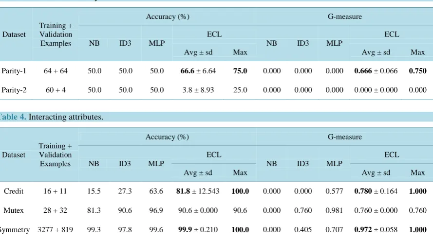
Two artificial datasets for parity problems, both with 6 Boolean attributes, were used in our first experiment. As can be seen in Table 3, even taking all the instance space as training set, no system was able to generalize good concept descriptions from the examples.

4.2. Interacting Attributes

An n-way interaction [4] is an interaction involving

(

n−1

)

attributes and a class label. Clearly, XOR is a kind of 3-way interaction; thus, concepts described in terms of interacting attributes tend to be harder to learn.

Table 3. Statistical neutrality.

Dataset

Training + Validation

Examples

Accuracy (%) G-measure

NB ID3 MLP

ECL

NB ID3 MLP

ECL

Avg ± sd Max Avg ± sd Max

Parity-1 64 + 64 50.0 50.0 50.0 66.6 ± 6.64 75.0 0.000 0.000 0.000 0.666 ± 0.066 0.750

[image:8.595.93.538.94.340.2]

Parity-2 60 + 4 50.0 50.0 50.0 3.8 ± 8.93 25.0 0.000 0.000 0.000 0.000 ± 0.000 0.000

Table 4. Interacting attributes.

Dataset

Training + Validation Examples

Accuracy (%) G-measure

NB ID3 MLP

ECL

NB ID3 MLP

ECL

Avg ± sd Max Avg ± sd Max

Credit 16 + 11 15.5 27.3 63.6 81.8 ± 12.543 100.0 0.000 0.000 0.577 0.780 ± 0.164 1.000

Mutex 28 + 32 81.3 90.6 96.9 90.6 ± 0.000 90.6 0.000 0.760 0.981 0.760 ± 0.000 0.760

Symmetry 3277 + 819 99.3 97.8 99.6 99.9 ± 0.210 100.0 0.000 0.405 0.707 0.972 ± 0.058 1.000

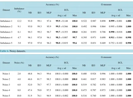
4.3. Imbalanced Datasets

Imbalanced datasets [5] are characterized by training sets with too few examples in one class and too many examples in the other one. This kind of dataset is very common, for example, in medical diagnosis applications, where a rare disease must be identified.

In our third experiment, we have used five imbalanced datasets, defining concepts over objects with 12 attributes, with minority class distribution spanning from 12.2% to 3%. All these datasets are composed by a training set with 492 examples and a validation set with 3604 examples. As Table 5 shows, ECL is very robust for imbalanced datasets, being the system with best performance in this experiment. Moreover, we can observe that, when we consider the g-measure, NB was the system with worst performance (showing that a high accura-cy does not necessarily mean a high performance). This can be explained by the fact that statistical methods tend to favor the majority class, ignoring the examples in the minority class. It is also interesting to notice that, in this experiment, ID3’s performance was better than MLP’s performance. Thus, it seems that majority class examples also have a greater influence in the training of neural networks.

4.4. Noisy Datasets

Noisy datasets [6] are characterized by training sets that have some incorrectly labeled examples. This kind of dataset is also common in real world applications where the example labels are defined by domain specialists.

In our fourth experiment, we have used five noisy datasets, defining concepts over objects with 15 attributes, with noisy class labels varying from 2% to 10%, equally distributed in both classes. All these datasets are com-posed by a training set with 1639 examples and a validation set with 1638 examples. As shown in Table 6, ECL is also robust in presence of noise. In fact, ECL was the system with best performance in this experiment. Moreover, both in terms of accuracy and g-measure, NB was the system with worst performance. It is also in-teresting to notice that, with noisy datasets, MLP seems to be better than ID3.

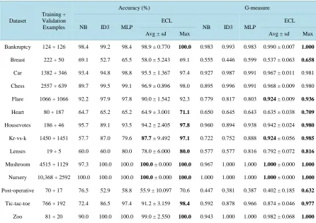
4.5. Natural Datasets

Natural datasets are datasets whose examples are collected from real-world applications, such as biological stu-dies, computer games, medical diagnosis, business operations, decision making, etc.

[image:9.595.90.538.96.424.2]

Table 5. Imbalanced datasets.

Dataset Imbalance (%)

Accuracy (%) G-measure

NB ID3 MLP

ECL

NB ID3 MLP

ECL

Avg ± sd Max Avg ± sd Max

Imbalance-1 12.2 91.0 99.1 97.4 99.9 ± 0.148 100.0 0.522 0.987 0.898 0.999 ± 0.001 1.000

Imbalance-2 9.1 93.0 99.3 95.9 99.5 ± 0.566 100.0 0.492 0.996 0.864 0.995 ± 0.006 1.000

Imbalance-3 6.1 94.3 99.2 96.7 99.7 ± 0.353 100.0 0.261 0.953 0.706 0.990 ± 0.018 1.000

Imbalance-4 4.7 96.1 97.8 96.1 98.3 ± 0.887 99.7 0.395 0.971 0.690 0.911 ± 0.064 0.998

Imbalance-5 3.0 97.0 97.0 96.2 98.0 ± 0.819 99.6 0.232 0.831 0.469 0.752 ± 0.102 0.998

Table 6. Noisy datasets.

Dataset Noise (%)

Accuracy (%) G-measure

NB ID3 MLP

ECL

NB ID3 MLP

ECL

Avg ± sd Max Avg ± sd Max

Noise-1 2.0 48.8 94.3 99.6 100.0 ± 0.000 100.0 0.480 0.924 0.996 1.000 ± 0.000 1.000

Noise-2 4.0 46.6 81.7 98.3 100.0 ± 0.000 100.0 0.461 0.817 0.983 1.000 ± 0.000 1.000

Noise-3 6.0 52.0 78.7 97.7 100.0 ± 0.000 100.0 0.519 0.782 0.976 1.000 ± 0.000 1.000

Noise-4 8.0 47.4 78.8 97.3 100.0 ± 0.000 100.0 0.473 0.787 0.973 1.000 ± 0.000 1.000

Noise-5 10.0 51.9 76.1 96.9 100.0 ± 0.002 100.0 0.516 0.760 0.969 1.000 ± 0.000 1.000

types of attributes used to describe the examples in the datasets, as well as the number of classes. Only datasets using nominal attributes were selected. Moreover, for datasets with more than two classes, one of them was randomly selected to be the positive class, and the remaining classes were collapsed to form the negative class.

The aim of this last experiment was to verify whether the system ECL can also have a good overall perfor-mance in practical applications. As can be observed in Table 7, our expectative was confirmed. In fact, ECL was the system with higher accuracies for the majority of the datasets (9 out of 14). Particularly, when we con-sider the g-measure as performance metric, ECL was the best system for almost all datasets (12 out of 14).

5. Conclusions

Concept learning is a kind of classification problem that has interesting practical applications in several areas and there are many distinct techniques that can be applied to solve this problem. However, it is well known that no single of such techniques is capable of solving all possible learning problems with high performance. Due to this fact, new approaches to machine learning are always welcome. In this paper, a new evolutionary algorithm to solve concept learning problems was proposed, and a corresponding learning system named ECL was imple-mented. The novelty in this algorithm is the fact that it combines ideas from different canonical evolutionary al-gorithms (i.e., genetic programming, evolutionary programming and evolution strategy).

[image:10.595.88.535.100.415.2]

Table 7. Natural datasets.

Dataset

Training + Validation Examples

Accuracy (%) G-measure

NB ID3 MLP

ECL

NB ID3 MLP

ECL

Avg ± sd Max Avg ± sd Max

Bankruptcy 124 + 126 98.4 99.2 98.4 98.9 ± 0.770 100.0 0.983 0.993 0.983 0.990 ± 0.007 1.000

Breast 222 + 50 69.1 52.7 65.5 58.0 ± 5.243 69.1 0.555 0.446 0.599 0.537 ± 0.063 0.658

Car 1382 + 346 93.4 94.8 98.8 95.5 ± 1.367 97.4 0.927 0.987 0.991 0.967 ± 0.011 0.981

Chess 2557 + 639 89.7 99.5 99.1 96.9 ± 0.896 98.0 0.895 0.996 0.991 0.968 ± 0.009 0.980

Flare 1066 + 1066 92.2 97.9 97.8 90.0 ± 1.542 92.3 0.779 0.817 0.803 0.924 ± 0.009 0.936

Heart 80 + 187 64.7 65.2 65.2 64.9 ± 3.001 71.1 0.650 0.645 0.643 0.635 ± 0.038 0.709

Housevotes 186 + 46 95.7 89.1 93.5 94.2 ± 2.405 97.8 0.960 0.894 0.938 0.942 ± 0.024 0.980

Kr-vs-k 1450 + 1451 57.7 87.0 79.6 87.7 ± 9.492 97.1 0.722 0.752 0.888 0.924 ± 0.056 0.985

Lenses 19 + 5 60.0 60.0 80.0 78.0 ± 6.000 80.0 0.577 0.577 0.816 0.792 ± 0.072 0.816

Mushroom 4515 + 1129 97.3 100.0 100.0 100.0 ± 0.000 100.0 0.967 1.000 1.000 1.000 ± 0.000 1.000

Nursery 10,368 + 2592 100.0 100.0 100.0 100.0 ± 0.000 100.0 1.000 1.000 1.000 1.000 ± 0.000 1.000

Post-operative 70 + 17 76.5 52.9 58.8 55.9 ± 10.097 70.6 0.447 0.381 0.387 0.402 ± 0.185 0.632

Tic-tac-toe 766 + 192 72.4 86.5 97.4 91.2 ± 3.159 98.4 0.592 0.878 0.966 0.874 ± 0.046 0.977

Zoo 81 + 20 90.0 100.0 100.0 99.0 ± 2.550 100.0 0.943 1.000 1.000 0.982 ± 0.068 1.000

learning repositories. The experiments performed with these datasets showed that ECL can also have a good overall performance in real world’s practical applications of concept learning. Thus, the main contribution of this paper was to offer a feasible alternative technique to solve classification problems in machine learning.

Some considerations also must be done about the higher ECL’s execution time. First, we observe that the learning of a specific concept is a task performed only once; on the other hand, the hypothesis learned is used many times. Thus, better hypotheses can justify higher execution times. Second, due to the inherent nondeter-minism of evolutionary approaches, when the user has more time available, by running ECL many times, he has the chance of obtaining better hypotheses. Clearly, the same is not true for the other compared machine learning approaches, which are deterministic and produce always the same hypotheses, from the same training set.

Finally, although the empirical evaluation performed has showed that the evolutionary approach proposed in this work has a good overall performance, we also would like to know whether it can be significantly better than other approaches. Thus, a natural extension of this work is to perform statistical tests with the obtained results.

Acknowledgements

This research is supported by CNPq (Brazilian National Counsel of Technological and Scientific Development), under grant numbers 305484/2012-5 and 103170/2014-6.

References

[1] Michie, D., Spiegelhalter, D.J. and Taylor, C.C. (1994) Machine Learning, Neural and Statistical Classification. Ellis Horwood, New York. http://www1.maths.leeds.ac.uk/~charles/statlog/whole.pdf

[2] Kotsiants, S.B., Zaharakis, I.D. and Pintelas, P.E. (2006) Machine Learning: A Review of Classification and Combin-ing Techniques. Artificial Intelligence Review, 26, 159-190. http://dx.doi.org/10.1007/s10462-007-9052-3

Poly-thechnique Fédérale de Lausanne, Lausanne. http://infoscience.epfl.ch/record/82654/files/rr00-46.pdf

[4] Menon, A.K., Agarwal, H.N.S. and Chawla, S. (2013) On the Statistical Consistency of Algorithms for Binary Classi-fication under Class Imbalance. Proceedings of the 30th International Conference on Machine Learning, Atlanta, 16- 21 June 2013, 603-611.

http://clweb.csa.iisc.ernet.in/harikrishna/Papers/Class-imbalance/icml13-class-imbalance.pdf

[5] Jakulin, A. (2003) Attribute Interactions in Machine Learning. M.Sc. Thesis, University of Ljubljana, Ljubljana.

http://www.stat.columbia.edu/~jakulin/Int/interactions_full.pdf

[6] Natarajan, N., Dhillon, I., Ravikumar, P. and Tewari, A. (2013) Learning with Noisy Labels. Advances in Neural In-formation Processing Systems, NIPS, 1196-1204. http://papers.nips.cc/paper/5073-learning-with-noisy-labels

[7] Whitley, D. (2001) An Overview of Evolutionary Algorithms: Practical Issues and Common Pitfalls. Information and Software Technology, 43, 817-831. http://dx.doi.org/10.1016/S0950-5849(01)00188-4

[8] Hekanaho, J. (1998) An Evolutionary Approach to Concept Learning. Ph.D. Thesis, Åbo Akademi University, Vasa.

http://citeseerx.ist.psu.edu/viewdoc/download?doi=10.1.1.27.6647&rep=rep1&type=pdf

[9] Thrun, S.B., et al. (1991) The Monk’s Problems—APerformance Comparison of Different Learning Algorithms. Technical Report, Carnigie Mellon University. http://people.cs.missouri.edu/~skubicm/375/thrun.comparison.pdf

[10] Labatut, V. and Cherifi, H. (2012) Accuracy Measures for the Comparison of Classifiers. Proceedings of the 5th In-ternational Conference on Information Technology, Chania Crete, 7-9 July 2014, 1-5.

http://arxiv.org/ftp/arxiv/papers/1207/1207.3790.pdf

[11] De Jong, K.A. (2006) Evolutionay Computation: A Unified Approach. MIT Press, London.

[12] Weise, T. (2008) Global Optimization Algorithms: Theory and Application. 2nd Edition. http://www.it-weise.de

[13] Koza, J.R. (1998) Genetic Programming. MIT Press, London.

[14] Fogel, L.J. (1964) On the Organization of Intellect. Ph.D. Thesis, University of California, Los Angeles.

[15] Rechenberg, I. (1965) Cybernetic Solution Path of an Experimental Problem. Royal Aircraft Establishment, Library Translation 1122, Farnborough.

[16] Witten, I.H., Frank, E. and Hall, M.A. (2011) Data Mining. 3rd Edition, Morgan Kaufmann, Burlington. [17] Ceder, V.L. (2010) The Quick Python Book. 2nd Edition, Manning Publications Co., Greenwich.

[18] Alcalá-Fdez, J., et al. (2011) KEEL Data-Mining Software Tool: Data Set Repository. Integration of Algorithms and Experimental Analysis Framework. Journal of Multiple-Valued Logic and Soft Computing, 17, 255-287.

http://www.keel.es

currently publishing more than 200 open access, online, peer-reviewed journals covering a wide range of academic disciplines. SCIRP serves the worldwide academic communities and contributes to the progress and application of science with its publication.

Other selected journals from SCIRP are listed as below. Submit your manuscript to us via either