Comparative Study of Three Different Path Tracking Controls in Mobile Robots

Comparative Study of Three Different Path Tracking

Controls in Mobile Robots

Abel García-B., Cristian

G. Pérez-T., Eduardo S.

Espinoza-Q., and

Francisco R. Trejo-M.

Department of Mechatronics, Polytechnic University of Pachuca, Zempoala, Hidalgo,

Mexico

Luis E. Ramos-V. and

Hugo Romero-T.,

Research Center for Information Technologies and

Systems, Autonomous University of Hidalgo State

(UAEH), Hidalgo, Mexico

Jesús M. Muñoz-P.

Department of Electronics, Meritorious Autonomous University of Puebla (BUAP),

Puebla, Mexico

ABSTRACT

This paper presents a comparative study of three different path tracking control laws for the formation of a group of nonholonomic mobile robots. By introducing a unified error of the formation and trajectory tracking using; the dynamic feedback linearization control [1], dynamic-static feedback linearization control [2] and nonlinear time-invariant control [3] are compared. The simulations results show that the dynamic-static feedback linearization technique presents a stable tracking with smoother behaviour and avoiding discontinuities for tracking trajectory of the robot leader. Finally, this method was implemented experimentally in three different paths formatting a simple triangle with three mobile robots in a leader-follower type motion. Moreover, the analysis in this paper reveals some important issues raising that the following control on this system can be extended to underactuated AUVs in future work.

Keywords

Multiple robot system; formation path tracking; nonlinear control law.

1.

INTRODUCTION

Over the last decades, a lot of attentions have been paid to research on the cooperative control and formation control of multiple robots, especially on mobile robots. The collective nature of multi robot systems attracts many vibrant real world applications. It includes exploration, surveillance, cooperative large objects, cooperative attack and rendezvous and formation control [1-8]. With increasing popularity and interest in the vision of multirobots systems, there are many topics with huge potential to make these mechatronics systems possible in real life applications [9]. There is currently considerable interest in the problem of coordinated motion control to carry out a specific task of cooperation, i.e. to move a heavy object. Different control strategies have been proposed [13], which include the behaviour based, virtual -structure, leader following, and graph theoretical approaches. While most existing results use linear vehicle dynamics to simplify control design, we study formation control of nonhomolomic mobile robots. Formation control means the problem of controlling the relative position and orientation of the mobile robots in a group according to some desired patter for executing a given task [10-11]. Trajectory tracking is required to enable the robot a time parameterized reference path. Path following drives the mobile robot to converge to a

follow a desired spatial path, without strict temporal specifications. Also, different approaches have been proposed and implemented to tackle the robot formation control problem [6-9]. Typically, smoother convergence to a path is achieved when path following strategies are used instead of trajectory tracking control laws, and the control signals are less likely pushed to saturation. The most common techniques used are the following: dynamic feedback linearization control [1], a dynamic-static feedback linearization control [2] and nonlinear time-invariant control [3]. The dynamic and dynamic-static feedback linearization techniques are used to derive the formation control laws for follower robots that are used for leader-following formation. The nonlinear time-invariant feedback control is another technique to carry out the formation of multi robots systems.

In this paper, we present the comparison of three different path-tracking controls for the formation of mobile robots. Nonlinear control laws to tracking paths on a Cartesian plane and maintaining the desired formations are simulated and implemented. The simulation path of the mobile robot is carried out by using the Matlab toolbox animation. The technique of input-output linearization by dynamic-static feedback control for trajectory tracking and formation control was implemented experimentally in this paper. The remainder of the paper is structured as follow. In Section II the kinematic models of nonholomic mobile robots are presented, in Section III the control laws compared in this paper are presented. Simulation and experimental results of the formation robots and path tracking are presented in Section IV. Finally, in Section V, we present the conclusions of this research.

2.

KINEMATIC MODELS

48 robots under study in this paper are made up of rigid frame

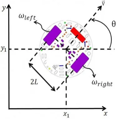
equipped with non-deformable wheels and they are moving on a horizontal plane. Figure 1 shows the schematic diagram of wheeled mobile robot with two driven wheels (in the rear part) and a passive castorwheel (in the front).

Figure 1: Schematic diagram of the mobile robot

The state-space model of the considered kinematic vehicle with the associated nonholonomic constraints (rolling with no slipping) is given by,

𝑥 =𝑟 𝜔𝑙𝑒𝑓𝑡 + 𝜔𝑟𝑖𝑔 𝑕𝑡 cos 𝜃

2 (1)

𝑦 =𝑟 𝜔𝑙𝑒𝑓𝑡+ 𝜔𝑟𝑖𝑔 𝑕𝑡 sin 𝜃

2 (2)

𝜃 =𝑟 𝜔𝑙𝑒𝑓𝑡− 𝜔𝑟𝑖𝑔 𝑕𝑡

2𝐿 (3) where r is the radius of the tire, L is the distance between the tire and the centre of the robot, ωleft and ωright are the angular

velocity of the left and the right wheel, respectively. The robot's position is completely specified by three variables x, y and θ, see Figure 1. Also, x1 and y1 represent the position

along the axis X and Y, respectively, and θ represents the orientation of the longitudinal axis of the robot with respect to the axis X. In matrix form, the velocities can be expressed as

𝑥 𝑦 𝜃

= cos 𝜃 0sin 𝜃 0

0 1

_𝜔𝑣1

1 (4) where v1 and ω1 are the linear and angular velocity,

respectively, and θ is the robot orientation, which represent the unicycle-type mobile robot model, the relations between v1, ω1 and ωleft, ωright are given by,

𝑣1 𝜔1 =

𝑟

2 𝑟 2

𝑟

2𝐿 − 𝑟 2𝐿

𝜔𝑙𝑒𝑓𝑡

𝜔𝑟𝑖𝑔 𝑕𝑡 (5)

In this paper, we consider a networked team of three nonholonomic unicycle-type mobile vehicles, labelled 1 trough 3, tracking a set of paths, while attaining a desired formation. First, we consider a two 3-wheel robot system, the coordinate positions of these two robots are shown in Figure2. It is a system of two mobile robots separated for a distance l12

between the centre of the first robot and the balance ball of the second robot, d denotes the distance between the balance ball and the axis of the wheels of each robot. The kinematics

equations, obtained from Figure 2, show that the system states variables are given by l12, ψ12, and θ2. Then, the kinematic

equations for a single robot are given by Eq. (4), while and kinematic model for two robots is given by

𝑙 12 𝜓 12 𝜃2

=

cos 𝛾1 − cos 𝜓12 0

1

𝑙12sin 𝜓12 1

0 0

_𝜔𝑣1 1

+

0 𝑑 cos 𝛾1

− 1 𝑙 sin 𝛾1 1

𝑙12𝑑 cos 𝛾1

0 1

_𝜔𝑣1

1 (6)

where γ1= θ1 + ψ12 - θ2. One can see the states variables to

control according to the kinematic Eq. (6), and then it is possible to get the proper control scheme.

Figure 2: Schematic diagram for two mobile robots

Below, we presented an approach for tackling the rigid formation control problem by employing the flatness property. An effective control strategy allows us to execute formation maneuvers, departing from the formation, splitting the formation, and merging into formation.

3.

MOBILE ROBOT CONTROL

In the path tracking control of mobile robots, a nonholomomic unicycle-type of wheeled vehicle follows a predefined spatial path, Xd = [x(t)d; y(t)d; θ(t)d]. In this work, we move a mobile

robot along three desire paths described by the following equations

𝑦 𝑡 𝑑1= 𝑥 𝑡 𝑑 (7a) 𝑦 𝑡 𝑑2= 𝑥3 𝑡 𝑑 (7b)

𝑦 𝑡 𝑑3= 𝑟2− 𝑥 𝑡 𝑑− 𝑎 2+ 𝑏 (7c)

where Eqs. (7) describe a straight line, a hyperbola, and a semicircle path, respectively. In Eq. (7c), a and b represent the origin point of the semicircle. Deriving Eqs. (7) with respect to time and substituting in (4), we found that the orientation angle is given by the following equations

𝜃 𝑡 𝑑1= arctan 𝐶

𝜃 𝑡 𝑑2= arctan 3𝑥2 𝑡 𝑑 (8)

where C is the relation between xd and yd. The next step is to

define x(t)d, which is given by

𝑥 𝑡 𝑑= 𝑎 sin 2𝜋_𝑃𝑡 (9)

Using Eq. (9), the mobile robot goes from the origin at x = 0, y = 0 to the point x = a, y = a3 m, then it returns to the origin and moves to the point x = -a, y = -a3 _{m, and finally it backs}

again to the origin point, in the case of the second path and it will be ending in P seconds.

Dynamic Feedback Control. In this method, it is developed a controller that linearizes the input – output system response. Considering u1 and u2 as control variables, x and y as output

variables [1], it is possible to represent the system in the standard form 𝑞 = 𝐴 𝜃 𝑢

𝑥

𝑦 = cos 𝜃 0sin 𝜃 0 𝑢1

𝑢2 = 𝐴 𝜃 𝑢1

𝑢2 (10)

One can see that the matrix 𝐴 𝜃 is singular for all values of x, y, and θ, therefore it would not be possible to linearize the system. For this reason, we need a new state variable ς and also a control variable, 𝑢 1, where the change of variables are 𝜍 = 𝑢 1 and 𝑢1= 𝜍. The new control variables 𝑢 1and u2 are

related with the output variables as follow

𝑥

𝑦 = cos 𝜃 𝜍 sin 𝜃 sin 𝜃 𝜍 cos 𝜃 𝑢 1

𝑢2 = 𝐴 𝜃, 𝜍 𝑢 1

𝑢2 (11)

If 𝜍 ≠ 0, then it is possible to rewrite the feedback system as follow

𝑢 1 𝑢2 = 𝐴

−1 _{𝜃, 𝜍} 𝑣1

𝑣2 (12)

the new control variables are v1 and v2 are given by

𝑣1 𝑣2 =

𝑥 𝑑− 𝑘𝑥1𝑒 𝑥− 𝑘𝑥0𝑒𝑥

𝑦 𝑑− 𝑘𝑦1𝑒 𝑦− 𝑘𝑥0𝑒𝑥 (13)

where the constants kxi and kyi represent the control gains,

which make the error tends to converge to zero, and the error functions are defined by ex = xd – x and ey = yd - y.

Dynamic-static Feedback Linearization Control. The control law in Eq. (12), clearly, it is not defined when 𝜍 = 0. For this reason, we need to propose an static feedback control law that linearizes the input - output system [2], but with the output variables x and θ. From Eq. (4) we can see that the control variables are related with the output variables as follow

𝑥

𝜃 = cos 𝜃 00 1 𝑢1

𝑢2 = 𝐴 𝜃 𝑢1

𝑢2 (14)

where the control variables v1 and v2 were proposed as

𝑢1 𝑢2 = 𝐴

−1 _{𝜃, 𝜍} 𝑣1

𝑣2 (15)

where the control variables v1 and v2 are defined as

𝑣1 𝑣2 =

𝑥 𝑑− 𝑘𝑥𝑒𝑥

𝜃 𝑑− 𝑘𝜃𝑒𝑥 (16)

where the constants kx and kθ are the control gains, which

make the error to converge to zero and the error functions are defined by ex = x - xd and eθ = θ - θd.

The control law, in Eq. (15), is not defined for 𝜃 = 𝑘𝜋 2, k = ±1; ±2; … as it grows out of control, and as mentioned before the control law, Eq. (12) is not defined when ς = 0, i.e. when the robot is at rest or when the path indicates to the robot, that

must it stops for a moment. For these reasons, we can say that the control laws are not defined globally, and switching control given by Eq. (12), and the Eq. (15) is employed to avoid discontinuities.

Nonlinear Time-Invariant Control. The tracking controller given by [3] was obtained from a Lyapunov based design as

𝑣 = 𝑣𝑑cos 𝜃𝑑− 𝜃 + 𝑘1 𝑥𝑑− 𝑥 cos 𝜃 + 𝑦𝑑− 𝑦 sin 𝜃 (17)

𝜔 = 𝜔𝑑+ 𝑘2𝑣𝑑sin 𝜃_𝜃 𝑑−𝜃

𝑑−𝜃 𝑦𝑑− 𝑦 cos 𝜃 − 𝑥𝑑−

𝑥 sin 𝜃 + 𝑘3 𝜃𝑑− 𝜃 (18)

where vd and ωd are defined by the following equations

𝑣𝑑= ± 𝑥 𝑑2+ 𝑦 𝑑2 (19)

𝜔𝑑=𝑦 𝑑𝑥 _𝑥 𝑑−𝑥 𝑑𝑦 𝑑

𝑑 2_+𝑦

𝑑2 (20)

A common technique to calculate the control gains is by using

𝑘1= 𝑘3= 2𝜍 𝜔𝑑2+ 𝑏𝑣𝑑2 (21)

𝑘2= 𝑏 (22)

with damping coefficient ς  (0,1) and b > 0.

4.

RESULTS

We carried out the comparative study of three control laws, described in the last section, and maintained a triangular formation. In this case, we chose the leader-follower technique, with a leader and two robots followers. We use a controller that linearizes the response input-output system, using a control law that gives exponentially convergent to the variables l12 and ψ12, between robots 1 and 2, and the

variables l13 and ψ13, between robots 1 and 3, with control law

defined by Eq. (24)

𝜔𝑖= cos 𝜆𝑑𝑙𝑖 𝛼𝑖𝑙1𝑖 𝜓𝑑1𝑖− 𝜓1𝑖 − 𝑣1sin 𝜓1𝑖 + 𝑙1𝑖𝜔1+ 𝜌𝑙𝑖sin 𝜆𝑙𝑖 (23)

𝑣𝑖= 𝜌𝑙𝑖− 𝑑𝜔𝑖tan 𝜆𝑙𝑖 (24)

where

𝜌𝑙𝑖=𝛼1 𝑙𝑑1𝑖−𝑙_{cos 𝜆}1𝑖 +𝑣1cos 𝜓𝑙𝑖

𝑙𝑖 (25) where γ1i = θ1 + ψ1i - θi, vi and ωi are the linear and angular

velocities for each follower robot for i = 2, 3. This leads the error dynamics in the variables l-ψ variables in the form

𝑙1𝑖= 𝛼𝑖 𝑙𝑑1𝑖− 𝑙1𝑖 (26) 𝜓 𝑙𝑖= 𝛼𝑖 𝜓𝑑𝑙𝑖− 𝜓𝑙𝑖 (27)

50 avoid this discontinuity. In the case of the nonlinear

time-invariant controller controller does not appear the discontinuity ς = 0, but the controller has a non smoother behavior, therefore the dynamic-static feedback control works efficiently because it has stable tracking, an smoother behavior and avoid the discontinuity ς = 0.

Figure 3: Simulation results of path tracking controllers

In order to obtain an efficiently path, we consider that the leader robot plans a trajectory given by the dynamic-static feedback controller and two follower robots which overall the leader realize a triangular formation. Figure 4 shows the leader robot performing a straight line path which goes from the origin at x = 0 m, y = 0 m to the point x = 0.5 m, y = 0 m, then it returns to the origin and moves to the point x = 0.5 m, y = 0 m, and finally it backs again to the origin, is the same for the two follower robots. In order to obtain a triangular formation, we chose ψ12 = 60º, l12 = 2d for the robot follower

1 and ψ13 = -60º, l13 = 2d for the robot follower 2, where d =

0.06 m is the distance between the castor and the center of the axes of the wheels. One can see a smoother behavior of the two follower robots, see Figure 4. Also, it is observed peaks in both paths, because the follower robots change of orientation maintaining the framework orientation in entire path.

Figure 4: Straight line trajectory of the leader robot with two follower robots which overall realize a triangular

formation

The second path of the leader robot is a hyperbolic trajectory showed in the Figure 5, which goes from x = 0 m, y = 0 m to the point x = 0.5 m, y = 0.12 m, then it returns to the origin and moves to the point x = -0.5 m, y = -0.12 m, and finally it comes back again to the origin. Figure 5 shows an efficiently

path of the leader robot with two follower robots which are maintaining the triangular formation along entire path, each follower robot changes of orientation when the leader robot comes back to the origin.

Figure 5: Hyperbolic trajectory of the leader robot with two follower robots which overall realize a triangular

formation

The last trajectory to follow by the leader robot is the semicircle showed in the Figure 6, which goes from x = 0 m, y = 0 m to the point x = 0.5 m, y = 0.4 m, then it returns to the origin and moves to the point x = -0.5 m, y = -0.4 m and finally, it comes back again to the origin. Figure 6 shows an efficiently semicircular path tracked by the leader robot with two follower robots, which are maintaining the triangular formation along entire path, proving that it can realize any efficiently trajectory at time the follower robot maintaining the desire formation.

Figure 6: Semicircular trajectory of the leader robot with two follower robots which overall realize a triangular

formation

51 this one. This is a simple computational technique working on

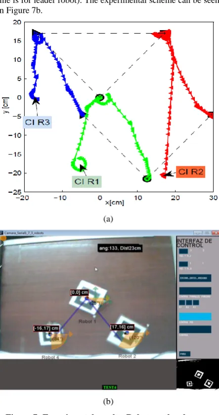
the pixel information of the image in comparison to other complex mathematical techniques available. The experimental results are showed in the Figure 7. One can see the trajectory for each robot and the triangular formation in Figure 7a (green line is for leader robot). The experimental scheme can be seen in Figure 7b.

(a)

(b)

Figure 7: Experimental results. Robots paths, they are keeping the triangular formation (a). Experimental

scheme shows the triangular formation too (b).

5.

CONCLUSIONS

A comparative study of three different path tracking control laws for the formation of a group of nonholonomic mobile robots has been carried out satisfactorily. The dynamic-static feedback linearization control technique presents the best performance on the trajectory following on kinematics robots with circle path and three different paths maintaining a simple triangular formation of multiple robots. The simulations and experimental results showed that this technique presents also a stable tracking with smoother behaviour and avoiding discontinuities for tracking trajectory of the robot leader. This analysis can be extended to underactuated AUVs in future work.

6.

ACKNOWLEDGMENTS

This project has been funded by the CONACyT-Mexico grant CB-169062 and also it has been partially funded by PROMEP: Redes Temáticas de Colaboración under the

project titled: Fuentes de Energías Alternas and by the ECEST-SEP (Espacio Común de Educación Superior Tecnológica) program under the mobility scheme for professors and students, and Jesús Manuel Muñoz-Pacheco thanks to VIEP-BUAP-2013 for the financial support.

7.

REFERENCES

[1] Gamage, G.W., Mann, G.K.I., Gosine, R.G., Formation Control of Multiple Nonholonomic Mobile Robots Via Dynamic Feedback Linearization, In Proceedings International Conference on Advanced Robotics, IEEE-ICAR 2009, pp. 1-6, 2009.

[2] Isidori A., Nonlinear control systems, 3rd Edition, Springer-Verlag, 1995.

[3] C. Samson, “Time-varying feedback stabilization of car-like wheeled mobile robots,” Int. J. of Robotics Research, vol. 12, no. 1, pp. 55-64, 1993.

[4] D. Rus, B. Donald, and J.Jennings, “Moving furniture with a team of autonomous robots,” in Proc. IEEE/RSJ IEEE. Int. Conf. Intelligent Robots and Systems, pp. 556– 561, 1995.

[5] M. Mataric, M. Nilsson, and K. Simsarian, “Cooperative multi-robot box pushing,” in Proc. IEEE/RSJ IEEE. Int. Conf. Intelligent Robots and Systems, pp. 235–242, 1995. [6] T. Balch and R. Arkin, “Behaviour-based formation control for multirobot systems,” IEEE Trans. on Robotics and Automation, vol. 14, no. 6, pp. 926–939, 1998.

[7] A. Das, R. Fierro, V. Kumar, J. Ostrowski, J. Spletzerm, and C. Taylor, “A vision-based formation control framework,” IEEE Trans. on Robotics and Automation, vol. 18, no. 5, pp. 813–825, 2002.

[8] W. Ren, “Consensus based formation control strategies for multivehicle systems,” In Proc. American Control Conference, June 2006.

[9] M.-Y. Chow, S. Chiaverini, and C. Kitts, “Guest Editorial introduction to the focused section on mechatronics in multirobot systems,” IEEE/ASME Trans. Mechatronics, vol. 14, no. 2, pp. 133–140, 2009

[10] R. M. Bhatt, C. P. Tang, and V. N. Krovi, “Formation optimization for a fleet of wheeled mobile robots-A geometric approach,” Robot. Auton. Syst., vol. 57, no. 1, pp. 102–120, 2009.

[11] M. Egerstedt and X. Hu, “Formation constrained multi-agent control,” IEEE Trans. Robotics and Automation, vol. 17, pp. 947–951, 2001.

[12] J. P. Desai, J. Ostrowski and V. Kumar, “Controlling formations of multiple mobile robots,” IEEE International Conference on Robotics & Automation, Belgium, 1998.

[13] M. S. Carlos et al., “Coordinated control of mobile robots based on artificial vision,” International Journal of Computers, Communication & Control, vol. 1, no. 2, pp. 85-94, 2006.