A New Quantization Factor Method based on Genetic Algorithm for Audio Compression

(1)

A New Quantization Factor Method based on Genetic

Algorithm for Audio Compression

Dhia A. Alzubaydi

College of Science, Al-Mustansiriya University

Baghdad-Iraq

Zinah S. Abduljabbar

College of Science, Al-Mustansiriya University

Baghdad-Iraq

ABSTRACT

Data compression techniques have a great importance in many applications; one of these compression techniques is audio compression which is widely used in applications such as audio transmission and storage so many forms of audio compression techniques have been investigated. The central point of the proposed system is using genetic algorithm to find appropriate quantization factor for each file instead of using quantization factor specified by user and this is done after using digital signal processing techniques based on Slantlet transform.

Keywords

Audio compression, Slantlet transform, Genetic algorithm.

1. INTRODUCTION

A rapid growth in the using of the internet and mobile telephones has been experienced this leads to several data compression schemes have been investigated for reducing storage space and communication capacity requirement. Data compression is one of the most important fields and tools in modern computing; it provides a comprehensive reference for the many various types and methods of compression [1]. Compression is the process of re-encoding digital data to minimize file size; a specialized program called a codec, for COmpressor/DECompressor, changes the original file to the smaller version and then decompresses it to again present the data in a usable form [2]. Audio compression is an application of data compression which is in high demand as it is reduces the cost in audio storage and internet bandwidth, compression techniques are used to represent the audio at a lower bit-rate without degradation the quality significantly [3]. Most signals in practice are time domain; mathematical transformations can be applied on these signals to obtain information which is not easily available from its original format, Slantlet transform is used in the proposed system for this purpose.

Genetic algorithms are adaptive methods that may be used to solve search and optimization problems. They are based on genetic processes of biological organisms described first by Charles Darwin in the origin of species. Populations of competing individuals evolve over many generations according to the principle of natural selection and "survival of the fittest" [4]. Genetic algorithm is used in this paper to improve the performance of the compression system by finding quantization factor for each file.

2. AUDIO COMPRESSION

Compression of audio signal has found application in many fields, such as multimedia signal coding, high fidelity audio for radio broadcasting, audio transmission for HDTV and audio data transmission / sharing through internet [5]. Any

compression technique belongs to either lossy compression or lossless compression; the aim of lossless compression is to encode the data in a way such that the matching decoder is able to reconstruct an exact copy of the original signals that are input to the encoder [6]. Lossless compression is used when it is important that the original and the decompressed data be identical, for example, it is used in popular ZIP file format and other examples are executable programs and source code. Lossy compression technique includes some loss of information and data that have been compressed using lossy techniques generally cannot be recovered or reconstructed exactly [7]. In digital audio coding, a lossy codec is also called a perceptual codec because the design principle of a lossy audio codec is to remove the perceptually irrelevant or unimportant information as much as possible [6]. Lossless and lossy compressions are not entirely isolated techniques. Most lossy algorithms make use of some lossless technique as part of the total compression process. Generally, once insignificant information has been discarded, the resulting data is more amenable to lossless compression [8]. In this paper lossy and lossless compression are used to perform compression process. There are many techniques that achieve superior compression performance (good quality at low-bit rate) by removing redundancies in an audio signal; there are types of redundancies [3]:

1.Statistical redundancy. 2.Temporal redundancy. 3.Knowledge redundancy.

4.Perceptual irrelevancies: In addition to the above techniques, the human auditory system properties can be exploited, “perceptual irrelevancies” present in the audio signals are exploited to reduce the amount of information. The errors that are introduced result from removal of those signal components that are perceptually irrelevant [9].

3. CODING CLASSIFICATION

Three types of coding can be used in compression process: entropy coding, source coding and hybrid coding [10]. 1.Entropy Coding: Entropy coding are “noiseless coding”

methods to design variable bit length codes that reduce the overall number of bits needed to transmit the coded signal [11]. It is lossless because the data prior to encoding is identical to the data after decoding; no information is lost, such as RLE, AC and huffman coding.

2.Source Coding: In this type there is a loss of data taking advantage of limits of eye and ear. There are various types of source coding techniques such as [5]:

a.Linear Predictive Coding (LPC).

(2)

d.Transform Coding.

e.Variance Fractal Compression.

3.Hybrid Coding: Most are combinations of entropy and source coding, hybrid techniques frequently used in the multimedia field.

4. SLANTLET TRANSFORM

SLT is an orthogonal DWT, with two zero moments and with improved time localization. The basis is not based on filter bank iteration; instead, different filters are used for each scale. In general the algorithm to obtain l -scales Slantlet filter banks is as follows [12]:

1.The l- scale filter bank has 2l channels. The low pass filter is to be called hl(n). The filter adjacent to the low pass channel

is to be called fl (n). Both hl (n) and fl(n) are to be followed by

down sampling 2l.

2.The remaining 2l -2 channels are filtered by gi (n) and its

shifted time-reverse gi ((2i+1 – 1)-n) for i=1… l -1, each is to be followed by down sampling by 2i+1.

In the Slantlet filter bank, each filter gi(n) appears together

with its time reverse. While hi (n) does not appear with its

time reverse, it always appears paired with the filter fi (n).

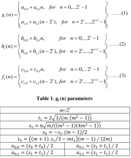
[image:2.595.326.498.95.263.2]

Figure (1) illustrates a three-scale Slantlet filter bank [12]. These filters gi (n), hi (n) and fi (n) for l-scale Slantlet are calculated using the following expressions and the parameters in tables (1) and (2) [12]:

Table 1. gi (n) parameters

[image:2.595.54.283.348.624.2]

m=2i

Table 2. hi (n) and fi(n) parameters

m=2i Note that the parameters a0,0 ,a0,1 ,a1,0 and a1,1 depend on i ,The same approach works for fi(n) and hi(n) . Using, again, a

piecewise linear form fi(n) and hi(n) can be written in terms of

eight unknown parameters b0,0 ,b0,1 ,b1,0b1,1,c0,0 ,c0,1 ,c1,0 and c1,1.

5. THE PROPOSED SYSTEM

A demonstration for suggest compression system will be presented using the following steps:

1. Loading audio file.

2.Framing process: in this step the channel is divided into number of non-overlapping frames, the size of each frame is 1024 samples and the last frame is padding with zeros if required.

3.Transformation process is applied on each frame using Slantlet transform. Genetic algorithm is applied on the copy of the transformed data.

4.In filtering process the threshold value is defined. In this paper adaptive threshold is established for each audio file, so the threshold value depends on Slantlet coefficients and this done by taking absolute value for all coefficients of the channel, computing the mean value for these coefficients and dividing the mean value by three. All Slantlet coefficients whose absolute values are equal or less than a certain threshold value are set to zero, while the other Slantlet coefficients are left. The outputs of filtering process are two vectors, the first vector for important coefficients and the other for their indexes.

5.Quantization process: uniform quantization is applied using appropriate quantization factor and the value of quantization factor is calculating using genetic algorithm. Quantization factor (QF) has a great impact on compression process; it limits the number of different symbols to be send from encoder to decoder side. QF is not an absolute value, for instance 400 may be appropriate QF for one file but for other one may affect the quality of the reconstructed file accordingly the compression system performance is improved by using GA to find an appropriate QF for each audio file. The uniform quantization is done by using the following equation:

The genetic approach is used to find appropriate QF, this is done by:

A. Representation for candidate solutions (binary coding is used to represent the chromosome).

B. The first generation is generated randomly, the size of population is equal to 50 chromosomes and the length of each chromosome is equal to10.

C. The most critical step in genetic algorithm process is determining the objective function which leads to find QF. QF inversely proportional with PSNR. PSNR is not an absolute value for all files; for instance a reconstructed file with specific value of PSNR has a bad quality other reconstructed ……(1)

…

(2.2)

                     1 2 ,..., 2 ), 2 ( 1 2 ,... 0 , ) ( 1 1 , 1 0 , 1 1 , 0 0 , 0 i i i i i n for n a a n for n a a n g                   _ 1 2 ,..., 2 ), 2 ( 1 2 ,... 0 , ) ( 1 1 , 1 0 , 1 1 , 0 0 , 0 i i i i i n for n b b n for n b b n h ……(2)

…

(2.2)

4

8

4

8

file with the same value of PSNR has a good quality. So there must be a way to determine the required value of PSNR for each file and this value is set as a fitness function and this is done through:

I.Calculate PSNR1 with QF=1 , this is mean that the values before quantization process equal to the values after de_quantization process except the decimal values that are lost due to the round process.

II.Calculate PSNR2 with QF=100 and find the difference between PSNR1 and PSNR2 (dPSNR), when the difference is small this means this file does not affected significantly by quantization process therefore QF may be large value. If the difference is big this means this file affected significantly by quantization process and QF should not be very large value to maintain the quality of the reconstructed file.

The computing of the Required PSNR is done by computing the difference between PSNR1 and the value resulting from multiplying the dPSNR by a specific factor (f) as follows:

Through several experiments to calculate the dPSNR value with different files, the lowest value obtained is 0.02 and this value is too small compared to other values of other files. When the difference is 0.02 then the factor is 28, for each increase by 0.01 of the difference value the factor is decreased by 1 and this is for each difference less than 0.2. When the difference is equal or greater than 0.2 then the factor is 10 so the equation to compute the factor:

the fitness function for each chromosome in the initial population is calculated and this is done by finding an equivalent decimal value for each chromosome, this decimal value is represent the QF and depending on this value (QF), PSNR is computed. The PSNR value is saved as a fitness function for the corresponding chromosome. So a fitness vector (FitPop) with size equals to the number of chromosome in the population is initialized.

D. After determining the fitness function (Required PSNR) three types of genetic operators that may be used in sequence and these are:

I.Triple tournament selection is used as a selection strategy in a proposed system which is operates on the bases of randomly choosing three chromosomes from the old population and selecting the fittest one from them. In each generation, the selection process is applied twice on the population to prepare two chromosomes (parents) for crossover and mutation. II.There are many methods to do crossover operation; single

point crossover is used with crossover probability equal to 1. Crossover point is determined randomly and all bits beyond that point in each chromosome are swapped, the resulting chromosomes are children.

III.Mutation is the last operation performed after crossover operation. This operation flips some of bits in a chromosome according to mutation rate. In the proposed system mutation rate is set to 0.05.

E. Two types of replacement in GA generational replacement and steady state replacement. The potential problem of the generational replacement is the risk of discarding some good individuals in the old generation, so steady state is used as a

strategy for replacement. A replacement/deletion strategy defines which member of the population is replaced by the new offspring; deleting the worst member of the old population is used, the new member is not inserted in the population unless be sure there is no member in the old population identical to the new one. This step ensures maintaining the good individuals in the population and prevents the case of repetition of individuals in the new population.

Stopping condition is satisfied when the difference between the Required PSNR and the PSNR of one individual in population is equal or less than 0.03 or when the maximum replacement equals to 100. After finding QF, quantization process is applied on Slantlet coefficients.

6.Differencing process is applied on the indexes vector and this done by keeping the first value of the given vector in a new vector while the other values of the new vector are resulting from subtraction the preceding from current value of a given vector.

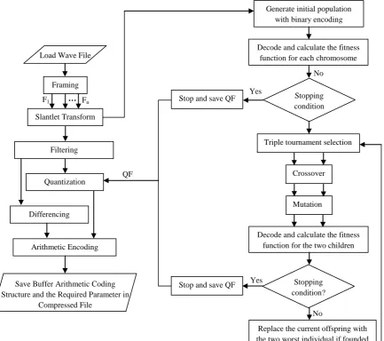
7.The quantized values with the outputs of differencing process are encoding using Arithmetic encoding. The steps for implementation encoding algorithm are shown in figure (2).

6. THE TEST MEASURES

The measures used in this paper to assess the performance of the considered compression method are the following:

6.1 The Fidelity Criteria

These measures (mean square error and peak signal to noise ratio) have been used to represent the level of the overall error caused due compression process. The adopted Fidelity measures could be defined as follows [13]:

…. (7) xn is the original signal.

yn is the reconstructed signal.

N is the total number of samples.

6.2 Compression Factor

A very logical way of measuring how well a compression algorithm compresses a given set of data is to look at the ratio of the number of bits required to represent the data before compression to the number of bits required to represent the data after compression [13]. This ratio is called the compression factor (CF); the compression factor is calculated by using the following equation [1]:

PSNR1-(dPSNR×f) when dPSNR<0.2

PSNR1-(dPSNR×10) when dPSNR ≥ 0.2

Required PSNR=

… (5)

…

(2.2)

..… (6)

…

(2.2)

f= 28-(dPSNR-0.02)×100 when dPSNR˂ 0.2

(4)

7. TEST RESULTS

To evaluate the performance of the proposed coder and the effects of the quantization factor on the quality of the reconstructed files, a test set including four files with different size (mono, 16 bits per sample and 44100 samples per second) are taken as test material.

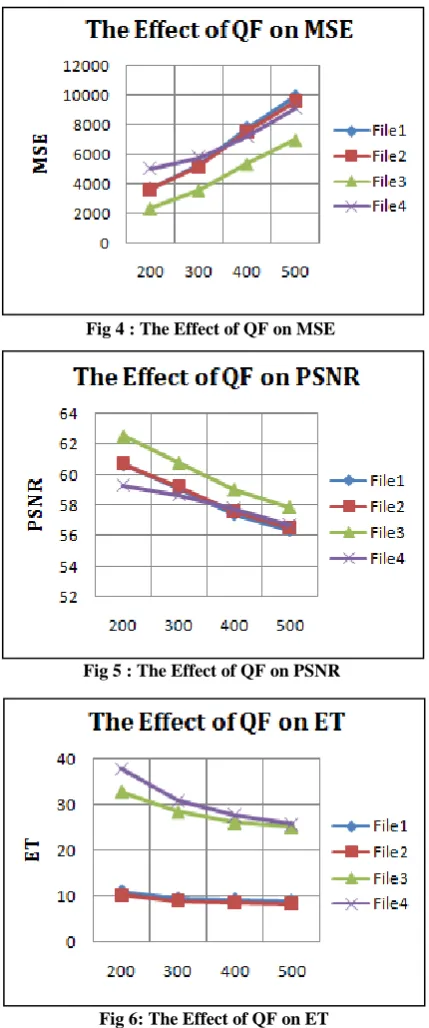
Quantization factor is the main critical parameter used in compression system, when QF increased the number of symbols of the audio file which are sent from encoder to decoder side are decreased. CF is increased significantly when QF is increased, MSE is proportional with CF and large QF may adversely affected the quality of the reconstructed audio file and decreased the time required for encoding and decoding processes. Figures below show the effects of different values (without GA) of QF for CF, MSE, PSNR, ET and DT respectively. So it’s useful to find appropriate QF for each file using genetic algorithm. Table (3) shows the duration, size, threshold value and QF for each file after performing genetic algorithm.

Generate initial population with binary encoding

Decode and calculate the fitness function for each chromosome

Stopping condition

Triple tournament selection

Crossover

Mutation

Decode and calculate the fitness function for the two children

Stopping condition? Stop and save QF

Replace the current offspring with the two worst individual if founded Stop and save QF

Save Buffer Arithmetic Coding Structure and the Required Parameter in

Compressed File Arithmetic Encoding

Framing

…

F1 Fn

Slantlet Transform

Quantization Filtering

Differencing Load Wave File

QF

Yes

No

[image:4.595.75.509.80.464.2]

No Yes

Fig 2: Functional Flow Diagram of Encoding Unit

[image:4.595.316.534.551.714.2]

(5)

Table 3. Specifications of the Tested Audio Files

File Duration (Sec)

Size (MB)

Threshold Value QF

File1 35 2.97 152 380

File2 33 2.8 157 380

File3 109 9.15 153 410

File4 93 7.8 222 400

Some performance measures are taken in the consideration to evaluate the performance efficiency of the suggested audio compression system. The adapted parameters are the fidelity criteria (MSE and PSNR), CF, encoding and decoding time. According to the QFs which are founded for each file, the results are listed in table (4).

Table 4. Results of Compression Process

File CF MSE PSNR

(dB) ET (Sec)

DT (Sec) File1 8.71 7319.59 57.68 10.04 3.24 File2 8.65 7084.15 57.82 8.97 3.02 File3 11.51 5534.86 58.89 28.61 11.04 File4 9.77 7230.77 57.73 27.69 9.95

Figure (8) shows the original and reconstructed signal “File2.wav”.

Fig 8. Original and Reconstructed Wave Forms of File2

8. CONCLUSIONS

1. SLT is an efficient transform for compression. 2. Quantization factor is a very important and critical

parameter in compression system.

[image:5.595.57.272.70.585.2]

Fig 5 : The Effect of QF on PSNR

Fig 6: The Effect of QF on ET

[image:5.595.319.536.72.240.2] [image:5.595.328.539.524.666.2]

(6)

3. GA with steady state replacement ensures finding an appropriate QF for each file.

4. Tournament selection scheme is an efficient and robust selection scheme in term of the efficiency to reach the optimum point in the defined search space.

5. Different QFs are found for different files with a high quality for the reconstructed files.

9. REFRENCES

[1] David S. , “The Compression The Complete Reference” Springer-Verlag London Limited (2007).

[2] Vogel K. E. and Savage T. M. , “An Introduction to Digital Multimedia”, by Jones and Bartlett Publishers, LLc (2008).

[3] Mrinal Kr. M. , “Multimedia Signals and Systems” Kluwer Academic Puplishers (2003).

[4] Xin Y. , “Evolutionary Computation: Theory and Applications” World Scientific Publishing Co. Pte. Ltd. (1999).

[5] Sheetal D. and Rajeshree D. R. , “Advance Source Coding Techniques for Audio/Speech Signal: A Survey” International Journal of Computer Technology and Applications (IJCTA), Vol.3 (4), July-August (2012).

[6] Dai T. Y. , Chris K. and C.-C. Jay K. , “High Fidelity Multichannel Audio coding” Hindawi Publishing Corporation (2006).

[7] Khalid S. , “Introduction to Data Compression”, Elsevier Inc (2006).

[8] Nigel C. and Jenny C. , “Digital Multimedia”, John Wiley & Sons, Ltd, Third Edition (2009).

[9] Jeroen B. and Christof F. , “Spatial Audio Processing: MPEG Surround and Other Applications”, John Wiley & Sons Ltd. (2007).

[10]Steinmetz R. and Nahrstedt K. , “Multimedia Fundamentals Volume 1: Media Coding and Content Processing”, Prentice Hall PTR (2002).

[11]Marina B. and Richard E. G. , “Introduction to Digital Audio Coding and Standards”, Kluwer Academic Publishers, Second printing (2003).

[12]Ivan S. “The Slantlet Transform” , IEEE Transaction on Signal Processing, Vol. 47, No. 5, pp. 1304-1313, May (1999).